Does the Opening of High-Speed Rail Change Urban Financial Agglomeration?

Abstract

High-speed rail (HSR) in China has led to altered spatiotemporal distances, thus inevitably affecting the regional economies. Has HSR also impacted the urban financial pattern? We analyze the relationship between HSR and financial agglomeration in 283 prefecture-level cities in China and find that HSR significantly reduces urban financial agglomeration and promotes financial diffusion. After the opening of HSR, financial employees (AGGE) and deposit agglomeration (AGGD) decrease by 0.06 and 0.07, respectively. Specifically: (1) HSR creates a financial diffusion effect by promoting industrial restructuring and technological innovation, thereby preventing excessive financial agglomeration in cities; (2) the heterogeneity analysis shows that financial factors are generally diffused from east to west, and HSR mainly causes a decrease in financial agglomeration in the eastern region; (3) we construct four spatial matrices for regression to further verify the impact of HSR, and we find that the indirect effect of HSR on financial agglomeration is more significant compared to the direct effect.

1. Introduction

Since 2008, China’s high-speed rail (HSR) has experienced rapid development, accounting for more than two-thirds of the world’s total mileage. In 2016, the “eight vertical and eight horizontal” network layout was proposed, marking China’s full entry into the “HSR era” (as shown in Figure 1). In the period of the “14th Five-Year Plan”, creating an “HSR economy” and laying out the passage network based on the advantages of HSR have become essential requirements for the achievement of high-quality economic development in China.Transportation infrastructure has proven to be an invaluable factor in economic growth [1]. HSR, as an efficient and comfortable means of passenger transportation, has changed China’s original spatial pattern and significantly reduced the spatiotemporal distances between regions [2]. Lu et al. (2013) find that within the two-hour economic circle of HSR, the access time can be halved [2]. This time and space compression effect of HSR can promote the economic growth of local and neighboring areas [3]. As the economy is closely related to finance, which plays a pivotal role as the core aspect of modern economic development, the impact of HSR on finance should not be ignored. In particular, talent, material, information, and capital, which are essential supports for regional economic activities, have experienced accelerated flows since the opening of HSR. Existing studies have mainly focused on changes in the first three factors under the impact of HSR. For example, Hu et al. (2020) find that HSR’s ability to facilitate commuting increases both urban employment and labor productivity, playing a critical role in alleviating the spatial mismatch of labor [4]. Sun et al. (2019) point out that although it is a means of passenger transport and cannot directly reduce the cost of goods, HSR has a substitution effect on roads and ordinary railroads within a certain range [5]. The freight capacity of other types of transport is reduced through passenger diversion, facilitating the flow of products and materials. Zhang et al. (2020) find that HSR can facilitate information flows and enhance enterprise monitoring [6]. However, little attention has been paid to how HSR affects the flow of funds.

The urban financial structure is crucial in supporting high-quality regional development and improving the country’s economic resilience [7,8,9]. In fact, the different attributes of the financial industry (or financial factors) and traditional manufacturing (or traditional factors) [10] may lead to contrasting effects of HSR. Therefore, it is necessary to separately examine the impact of high-speed rail on the financial industry. For example, Guan and Hu (2023) found that HSR had a significant agglomeration effect on the urban logistics industry and labor force [11]. Han et al. (2023) found that HSR significantly promoted population agglomeration [12]. Chen et al. (2024) found that HSR promoted regional industrial agglomeration, thereby facilitating green and sustainable development [13]. However, at the same time, it has been found that HSR has lagging and spillover effects on green development. This eventual spillover cannot be explained by the agglomeration of real industries. Kwilinski et al. (2023) suggested that economic spillover effects largely depend on financial spillover [14]. Compared with traditional factors, Huang et al. (2024) suggested that HSR mainly produces significant spillover effects on intangible factors represented by knowledge spillover [15]. Kwilinski et al. (2023) found that the spillover of this knowledge element will lead to the spillover of funds and the expansion of the scope of investment [14]. In addition, Wang et al. (2023) found that firms with distant customers tend to hold more cash due to precautionary motives [16], and the connectivity provided by HSR can reduce the risk of distant customers, thereby preventing firms from holding excessive amounts of cash. Thus, ignoring the differences between the financial industry and the real industry may lead to an incomplete analysis of the effects of HSR. Therefore, considering the shortcomings of existing research on the relationship between HSR and urban finance, this study focuses on analyzing the impact of HSR on urban finance from the perspective of financial agglomeration, thereby providing a more comprehensive framework for the analysis of HSR’s effects.

This study provides three marginal contributions to the existing literature. First, we explore whether HSR changes the existing urban financial landscape and affects the capital flows across regions by constructing indicators of urban financial agglomeration. Second, we further analyze the mechanisms based on the impact of HSR on financial agglomeration, particularly in regional innovation. We collect all granted invention patents in China covering the period from 2005 to 2018, analyze the citation and patentee address information, and finally aggregate it to construct patent–citation variables, effectively measuring the urban knowledge spillover. Third, we further explore the spatial effects of HSR by constructing different weight matrices.

The rest of this paper is organized as follows: Section 2 presents the literature review; Section 3 describes the variables and empirical models; Section 4 presents the basic regression results and a series of robustness tests; Section 5 further examines the influence mechanisms, heterogeneity, and spatial effects; Section 6 provides the conclusions and policy recommendations.

2. Literature Review

Transportation infrastructure is a critical factor for economic growth [1], with rail construction being particularly effective in promoting economic development and enhancing the capital market efficiency [17]. The opening of high-speed rail (HSR) leads to a reduction in transportation costs, driving regional employment and investment [5]. Vickerman (1997) finds that HSR can boost the economic growth of large cities [18], and this finding is verified by many scholars [19,20].

In recent years, many scholars have incorporated geographical factors into urban studies, forming the New Economic Geography. They have analyzed the relationship between agglomeration effects and economic development from a spatial perspective and propose that economic agglomeration can drive economic growth. Financial activities are closely related to economic activities, and the agglomeration effect of the financial industry is more significant compared to that of the manufacturing industry [21]. Financial agglomeration, as a specific type of industrial agglomeration, is the result of the constant evolutionary integration of various elements [22]. Its role in promoting economic growth will be revealed in the long run [23]. Currently, well-developed infrastructure is a necessary condition for financial centers [24]. Nicolae (2015) finds that geographical factors, represented by economic power, the labor force, and infrastructure power, have a positive impact on local financial development [25]. Ding (2018) includes road miles in an empirical analysis and highlights the importance of transportation infrastructure construction on financial development [26]. Wang et al. (2020) find that transportation infrastructure plays a critical role in financial agglomeration [27]. Using provincial panel data for spatial regression, they find that both roads and rail have a significant impact on financial agglomeration, but their effects are different.

Financial geography emphasizes that regional financial activities are significantly influenced by their geographical characteristics [28]. The opening of HSR has reshaped the spatial pattern, connecting previously isolated areas with the core areas [2]. HSR has improved the transportation infrastructure, expanded the coverage of financial institutions, reduced geographical information frictions, and changed the “local preference” of institutional investors [27]. The spatiotemporal compression of the “shrinking continent” will further affect the economic geography [29], and this change will impact regional financial agglomeration. Based on this, we propose Hypothesis 1 (H1).

H1. 

The opening of HSR will impact urban financial agglomeration.

The siphon and diffusion effects of HSR coexist [30]. On the one hand, the improved transportation infrastructure resulting from the opening of HSR promotes the transfer of material, talent, capital, and other resources to HSR cities [31], leading to the “siphon effect” [20]. Chen et al. (2024) suggest that the opening of HSR has promoted regional industrial agglomeration [13]. On the other hand, HSR expands the market boundaries and urban service areas, changing the local preferences of institutional investors [27] and creating a “diffusion effect” in HSR cities, which facilitates balanced regional development [32]. For instance, Li et al. (2016) find that the opening of HSR promotes economic growth in the western region, thereby reducing regional disparities [33]. By accelerating the flow of people, logistics, information, and capital, HSR strengthens regional cooperation and exchange, improves communication efficiency, and further expands the spillover of economic activities from central cities. Wang and Zhang (2023) find that the establishment of new HSR stations has led to the flattening of the economic density gradient of prefecture-level cities in China and promoted urban expansion [34]. Chen et al. (2023) find that the launch of HSR has greatly narrowed the inter-county economic gap and contributed to balanced regional development [35]. Reflected in the financial dimension, the siphon effect and diffusion effect of HSR jointly determine the direction of the change in urban financial agglomeration. When the development of transportation infrastructure is uneven, the mismatch of resources between regions is aggravated [36]. The improved transportation infrastructure shortens travel times and enhances the opportunities for face-to-face communication between lenders and borrowers, facilitating the transmission of “soft information” and expanding the reach of financial institutions in and around the region. Simultaneously, HSR facilitates cross-regional labor mobility, reduces the cost of face-to-face communication, improves the communication efficiency, and reduces information costs. By alleviating the information asymmetry between regions, HSR also helps to reduce the risks of financial transactions [37]. It can accelerate the cross-regional flow and rational allocation of funds and avoid the formation of financial bubbles due to excessive concentration. For example, Zhao et al. (2018) find that the risk of a stock price collapse in HSR cities appeared to decline significantly after the opening of HSR [37]. Wang et al. (2023) find that firms with long-distance customers tend to hold more cash due to precautionary motives and that HSR connectivity can reduce the impact of long-distance customers, thus preventing firms from holding excessive amounts of money due to these precautionary motives [16]. The following two opposing hypotheses are proposed regarding Hypothesis 1.

H1a. 

After the opening of HSR, urban financial agglomeration increases, indicating that the financial siphon effect of HSR is greater than the financial diffusion effect.

H1b. 

After the opening of HSR, urban financial agglomeration decreases, indicating that the financial diffusion effect of HSR is greater than the financial siphon effect.

On the one hand, HSR increases the frequency of face-to-face communication, facilitating the transfer of “soft information” between regions. This helps to expand knowledge spillover, strengthen knowledge and technology accumulation, and promote regional innovation [38]. Through innovation, new value depressions are formed, attracting capital inflows and thus changing the urban financial development pattern. First, high-value-added innovation activities often rely on face-to-face communications [39]. The form of face-to-face communication greatly enhances the communication efficiency, and the “soft information” that it creates alleviates the information asymmetry in socioeconomic production and exchange processes. By promoting face-to-face communication, HSR stimulates knowledge spillover and strengthens the “learning effect” of innovative subjects. By learning from advanced knowledge, experience, and technology, cities engage in imitative innovation and promote the development of innovative products [40]. In addition, the mobility of innovation resources increases with the improvement in urban accessibility [41]. By accelerating the flow of innovation factors such as the labor force, HSR optimizes the allocation of innovation resources and reduces the distance-related friction in knowledge and technology dissemination, thus improving the efficiency of innovation resource allocation and urban innovation. Second, technological innovation is a knowledge-intensive process, which makes it inherently complex, and it is difficult for a single individual or entity to complete the entire process alone [40]. The development of high-speed rail (HSR) networks can foster inter-regional communication and collaboration, allowing innovation stakeholders to jointly overcome challenges and promote regional innovation. Third, HSR expands the market scale, thereby intensifying market competition and motivating innovation stakeholders to continually enhance their technological processes and engage in research and development (R&D) innovation to remain competitive [40]. Overall, HSR drives both “hardware” and “software” improvements in innovation [41], deepening cooperation and promoting scale effects. This leads to the expansion of the service scope and boundaries of cities and creates a diffusion effect. With the widespread diffusion of knowledge and technology, as well as the reduction in information asymmetry, HSR provides more options for investment capital. The value discovery ability of capital increases, and the cost of mobility decreases, thereby enabling the outward diffusion of capital from HSR cities. Therefore, HSR drives the rational allocation of capital across a larger range by promoting technological innovation, thereby avoiding excessive capital accumulation.

On the other hand, advanced transportation facilities can have an impact on the regional industrial structure [27]. HSR accelerates the factor flow and generates labor division effects through resource integration, which helps to optimize the regional structure and upgrade the industrial structure [42]. As a result, industrial structure upgrading inevitably leads to adjustments in the financial structure [43]. The reallocation of financial resources has a ripple effect on urban financial agglomeration. According to Wang et al. (2020) [27], the adjustment, transformation, and upgrading of the industrial structure due to HSR will affect the spatial layout of the financial industry, driven by variations in industrial characteristics and financing preferences. Gong et al. (2014) also find that industrial development creates a demand for financing; with economic development [43], the industrial structure undergoes continuous upgrading, leading to changes in the financial structure. Chen et al. (2024) found that the opening of HSR can reduce environmental pollution through industrial structure adjustment and technological progress [44]. Nie and Zhang (2024) found that HSR promotes the rapid development of low-carbon industries through structural transformation effects [45].

The division effect of HSR refers to the development of industries among HSR-connected cities according to their comparative advantages and industrial development through trade [46]. Hu and Xu (2020) indicate that the industrial upgrading of HSR cities and the labor division effect collectively lead to industrial diffusion, where regions with a more backward industrial structure can take over industries from other cities by utilizing their comparative advantages, or they may further develop advantageous industries through knowledge spillover and technology exchange [47]. First, large cities can use their advantages in technology and talent concentration to focus on technology-intensive industries, such as high-end manufacturing or productive services, including electronic information and finance, while shifting labor- and capital-intensive manufacturing to smaller cities, where the labor and land costs are relatively lower. Second, firms can locate their R&D, management, and sales departments in large cities with strong knowledge and a dense consumer base to facilitate business expansion and customer visits, while shifting their production departments to small- and medium-sized cities [48]. This division effect applies to both consumer and production factor markets, with the costs of production factor transfer and information flows being the main obstacles to the division between regions. The emergence of HSR effectively reduces the cost of transferring labor and information between cities, breaking the spatial barriers to face-to-face communication and accelerating the division of labor and specialization across regions [49]. Moreover, Wang et al. (2020) argue that a bank-based financial system is crucial in the manufacturing-led stage [27]. With the accelerated transformation and upgrading of the secondary industry to the tertiary industry in HSR cities, the manufacturing industry gradually shifts to the surrounding cities. Accordingly, the capital also follows the diffusion of the manufacturing industry to continuously flow outward. This enables the allocation of idle funds saved in HSR cities to a wider range and reduces the concentration of idle funds in these cities. Ma et al. (2020) find that the number of investments by listed companies in non-local cities increases significantly after the implementation of HSR. Based on these findings [50], we propose Hypothesis 2 (H2).

H2a. 

HSR changes urban financial agglomeration by promoting regional innovation.

H2b. 

HSR changes urban financial agglomeration by promoting industrial structure upgrading.

3. Variables and Model

According to H1 and H2, we construct a series of regression variables and econometric models to empirically test the hypotheses.

3.1. Variable Selection

We use China’s 283 prefecture-level cities from 2005 to 2018 for the empirical analysis. The data sources are railroad train schedules and the China City Statistical Yearbook. The HSR opening in the first half of the year is considered as opening in the present year, while that opening in the second half of the year is considered as opening in the next year. We employ the location quotient index of financial employees and household saving deposits as the dependent variable to measure urban financial agglomeration. The specific calculation methods are as follows:

$$AGG{E}_{i,t}=\frac{F{E}_{i,t}/E_{i,t}}{{\displaystyle \sum _{i=1}^{n}F{E}_{i,t}/{\displaystyle \sum _{i=1}^n{E}_{i,t}}}}$$

(1)

where FE_i,t is the number of financial employees in city i in year t and E_i,t is the amount of total employment in city i in year t. Similarly,

$$AGG{D}_{i,t}=\frac{D_{i,t}/P_{i,t}}{{\displaystyle \sum _{i=1}^n{D}_{i,t}/{\displaystyle \sum _{i=1}^n{P}_{i,t}}}}$$

(2)

where $D_{i,t}$ is the household saving deposits in city i in year t, and $P_{i,t}$ is the total population in city i in year t. Larger values of ${AGGE}_{i,t}$ and ${AGGD}_{i,t}$ indicate a higher degree of financial agglomeration.

The core independent variable is the HSR opening dummy variable (HSR), which takes 1 for opening and 0 otherwise. We select the level of economic development (GDP), highway passenger traffic (PAS), the population growth rate (POP), the level of human capital (EMP), foreign direct investment (FDI), and the level of government regulation (GOV) as control variables, as shown in

Table 1. Variable descriptions.

Variable	Measurement	Observations	Mean	Standard Deviation	Min	Max
Urban financial agglomeration (AGGE)	Measured using the location quotient of financial employees	3914	1.0505	0.4098	0.1283	3.7625
Urban financial agglomeration (AGGD)	Measured using the location quotient of household saving deposits	3949	0.9949	1.0647	0.0202	14.9231
HSR opening (HSR)	If the HSR opens in the first half of the year, it takes the value of 1; otherwise, it takes the value of 0	3962	0.2845	0.4512	0	1
Economic development level (GDP)	Using 2003 as the base period for deflation, we obtain the GDP as constant prices (unit: CNY 1 billion)	3962	583.439	849.1944	8.6300	8594.93
Highway passenger traffic (PAS)	Measured using the urban highway passenger volume (unit: 10,000 people)	3932	8115.325	13,909.9	56	286,557
Population growth rate (POP)	Measured using the urban natural population growth rate (unit: %)	3936	5.8812	5.5671	−16.64	113
Human capital level (EMP)	Measured using the proportion of urban financial employees (unit: %)	3914	0.0039	0.0036	0.0001	0.0443
Foreign direct investment (FDI)	According to the China–US exchange rate published in the China Statistical Yearbook, the foreign direct investment in the city is converted into RMB (unit: CNY 10,000)	3746	552,051.5	1,389,276	0	2.05 × 107
Government regulation (GOV)	Measured as the proportion of local government expenditure to GDP (unit: %)	3954	0.2022	0.2213	0.0154	6.0406

.

3.2. Econometric Model

This study examines the impact of HSR on urban financial agglomeration by using the variable HSR as a difference-in-differences (DID) term. The conventional DID model is typically utilized to assess the impact of policy implementation at the same point in time. However, given the gradual nature of HSR deployment, we adopt a DID model for the regression analysis. Based on the results of the Hausman test, we construct a two-way fixed effects model that accounts for both city and year fixed effects. The model is as follows:

$$AGG{E}_{i,t}=\alpha +\beta HS{R}_{i,t}+\varphi X_{i,t}+{\lambda }_t+{\delta }_i+{\epsilon }_{i,t}$$

(3)

$$AGG{D}_{i,t}=\alpha +\beta HS{R}_{i,t}+\varphi X_{i,t}+{\lambda }_t+{\delta }_i+{\epsilon }_{i,t}$$

(4)

where i represents the city; t represents the year; ${AGGE}_{i,t}$ represents the financial agglomeration of city i in year t measured using the number of financial employees; ${AGGD}_{i,t}$ represents the financial agglomeration of city i in year t measured using the household saving deposits; ${HSR}_{i,t}$ is a dummy variable indicating whether city i opens high-speed rail in year t, with a value of 1 for opening and 0 for no opening. A positive coefficient $\beta$ indicates that the HSR opening causes urban financial agglomeration to increase. A negative coefficient $\beta$ indicates that the HSR opening decreases urban financial agglomeration. $X_{i,t}$ are control variables. We take the natural logarithm for all non-percentage variables to reduce the disturbance of extreme values; ${\lambda }_t$ represents year fixed effects; ${\delta }_i$ represents city fixed effects; ${\epsilon }_{i,t}$ is the error term. Considering that HSR’s impact may have a lag effect [3], we also use the HSR opening variable with a one-year lag (${\mathrm{H}\mathrm{S}\mathrm{R}\_1}_{i,t-1}$) in the regression.

4. Results

We conduct an empirical analysis based on econometric models (3) and (4) and conduct a series of robustness tests.

4.1. Basic Regression

To examine the impact of HSR on urban financial agglomeration, regressions are conducted based on the models of Equations (3) and (4), respectively, and the results are shown in columns (1)–(2) in

Table 2. Basic regression results.

	AGGE	AGGD	AGGE	AGGD
	(1)	(2)	(3)	(4)
HSR	−0.0586 ** (−2.52)	−0.0742 * (−1.96)
HSR_1			−0.0758 *** (−2.85)	−0.1107 *** (−2.80)
Control	yes	yes	yes	yes
Constant	1.1498 *** (3.16)	1.2968 ** (2.34)	1.1574 *** (3.20)	1.3205 ** (2.37)
City fixed effect	yes	yes	yes	yes
Year fixed effect	yes	yes	yes	yes
Observations	3853	3843	3853	3843

Note: Robust t-values are given in parentheses. *, **, *** represent p-values less than 0.1, 0.05, 0.01, respectively. The same applies in the following table.

. Due to the possible lagged effect of HSR, we also treat the core explanatory variable HSR with a one-period lag ($\mathrm{H}\mathrm{S}\mathrm{R}\_1$) and reperform the regression. The results are shown in columns (3)–(4) in Table 2.

The regression results in Table 2 (columns (1)–(2)) show that the coefficients of the variable HSR are significant at the 5% and 10% levels, respectively. In other words, H1 is validated, indicating that HSR changes urban financial agglomeration and affects the distribution pattern of the financial industry. Specifically, HSR has a significant negative impact on financial agglomeration. The degree of financial agglomeration in China’s cities decreases significantly after the opening of HSR, and the financial diffusion effect generated by HSR is generally larger than the financial siphon effect. As shown in columns (3)–(4), the effect of HSR on urban financial agglomeration is enhanced after a one-year lag treatment. The regression coefficient of the variable $\mathrm{H}\mathrm{S}\mathrm{R}\_1$ is significantly negative at the 1% level and the magnitude increases compared to columns (1)–(2), further indicating that HSR reduces urban financial agglomeration and there is a certain time lag in its effect. This result is consistent with the findings of Zhao et al. (2018), indicating that HSR can reduce the risk of a stock price collapse, thus contributing to the development goal of achieving inclusive finance [37]. Therefore, the regression results mainly confirm H1b in the opposing hypothesis. In other words, the financial diffusion effect of HSR is greater than the financial siphon effect.

4.2. Endogeneity

Considering that the regressions presented in Table 2 may possess endogeneity, which leads to biased coefficient estimates, we further conduct 2SLS and GMM regression analyses by constructing instrumental variables.

The geographic slope reflects the urban topographic condition, which affects the cost of building HSR. Since the geographic slope does not change during the sample period, the product of the geographic slope and year dummy variables for each city are included in the regression model as instrumental variables. In addition, historical railway data are exogenous and are correlated with HSR construction. They reflect a city’s historical transportation hub status. Therefore, referring to the methods of Dong et al. (2020) and Niu et al. (2020), we use historical railways and the average geographical slope as instrumental variables for HSR opening to conduct endogeneity tests [51,52]. Specifically, we multiply the number of urban railroad passengers in 1984 by the number of HSR cities in different years in the province where the prefecture-level city is located, and these are also included in the regression model as instrumental variables.

The first-stage 2SLS regression results show that the instrumental variables constructed using the geographical slope are negatively correlated with HSR opening; the higher the urban geographical slope, the higher the difficulty and cost of HSR construction and the more unfavorable it is to open HSR. In contrast, the urban historical passenger volume is positively correlated with HSR opening, i.e., cities with a higher historical passenger volume are more likely to open HSR. Overall, the F-values of all regressions in the first stage are significant at the 1% level, reflecting the correlation between the potential endogenous variables and instrumental variables. Meanwhile, the Kleibergen–Paap rk LM statistics for the unidentifiable test are all significant at the 1% level, and the Cragg–Donald and Kleibergen–Paap rk Wald F statistics for the weak instrumental variables test both exceed the standard value at the 10% level, indicating that the regressions do not suffer from weak instrumental variables. The Hansen J statistic for the overidentification test is also not significant. These results all indicate that the instrumental variables constructed are effective. As shown in

Table 3. 2SLS regression results.

	AGGE	AGGD	AGGE	AGGD
	(5)	(6)	(7)	(8)
HSR	−0.1304 *** (−2.69)	−0.3016 *** (−3.02)
HSR_1			−0.1599 *** (−3.31)	−0.3657 *** (−3.74)
Control	yes	yes	yes	yes
City fixed effect	yes	yes	yes	yes
Year fixed effect	yes	yes	yes	yes
Observations	2422	2422	2422	2422
Kleibergen–Paap rk LM	126.970	126.970	128.454	128.454
Cragg–Donald Wald F	12.877	12.877	13.483	13.483
Kleibergen–Paap rk Wald F	12.358	12.358	12.726	12.726
Hansen J	13.220	10.959	9.614	7.617

*** represent p-values less than 0.01.

, the regression coefficients of the core explanatory variables, $\mathrm{H}\mathrm{S}\mathrm{R}$ and $\mathrm{H}\mathrm{S}\mathrm{R}\_1$, remain significantly negative after employing the instrumental variables, and their magnitude and significance levels are increased compared to those in Table 2. In addition, in order to enhance the robustness of the instrumental variable regression, we use the GMM method for testing. The results are shown in

Table 4. GMM regression results.

	AGGE	AGGD	AGGE	AGGD
	(9)	(10)	(11)	(12)
HSR	−0.1401 ***	−0.2769 *** (−3.28)
HSR_1			−0.1653 *** (−3.46)	−0.3216 *** (−3.67)
Control	yes	yes	yes	yes
City fixed effect	yes	yes	yes	yes
Year fixed effect	yes	yes	yes	yes
Observations	2422	2422	2422	2422
Kleibergen–Paap rk LM	126.970	126.970	128.454	128.454
Cragg–Donald Wald F	12.877	12.877	13.483	13.483
Kleibergen–Paap rk Wald F	12.358	12.358	12.726	12.726
Hansen J	13.220	10.959	9.614	7.617

*** represent p-values less than 0.01.

; the coefficient is still significantly negative, and the conclusion remains unchanged.

4.3. Robustness

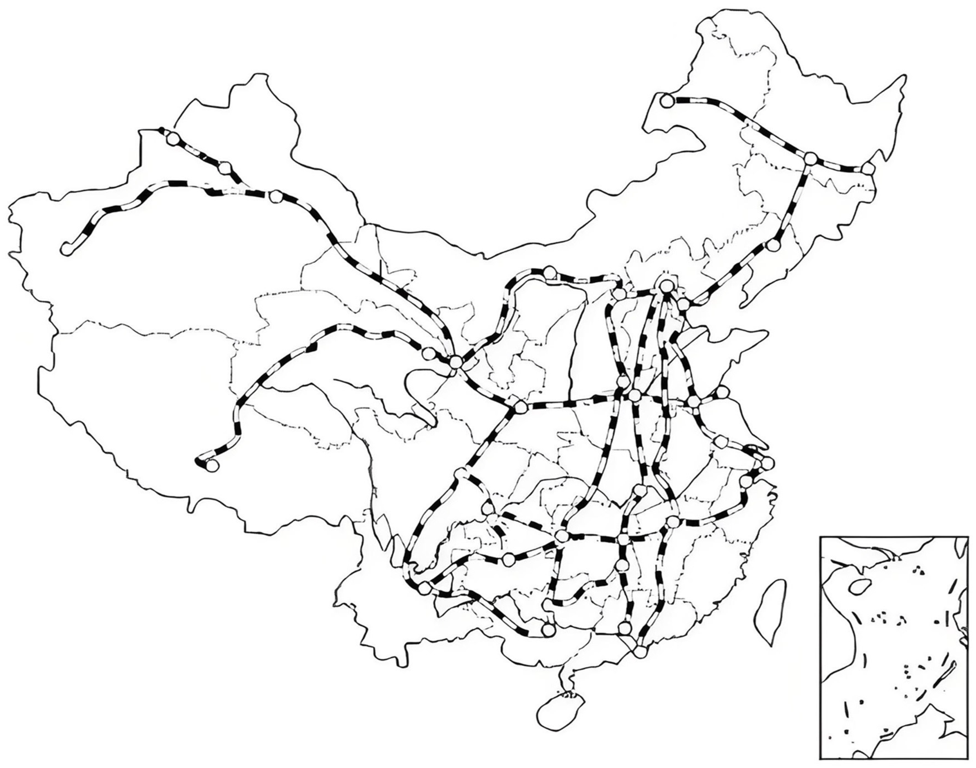
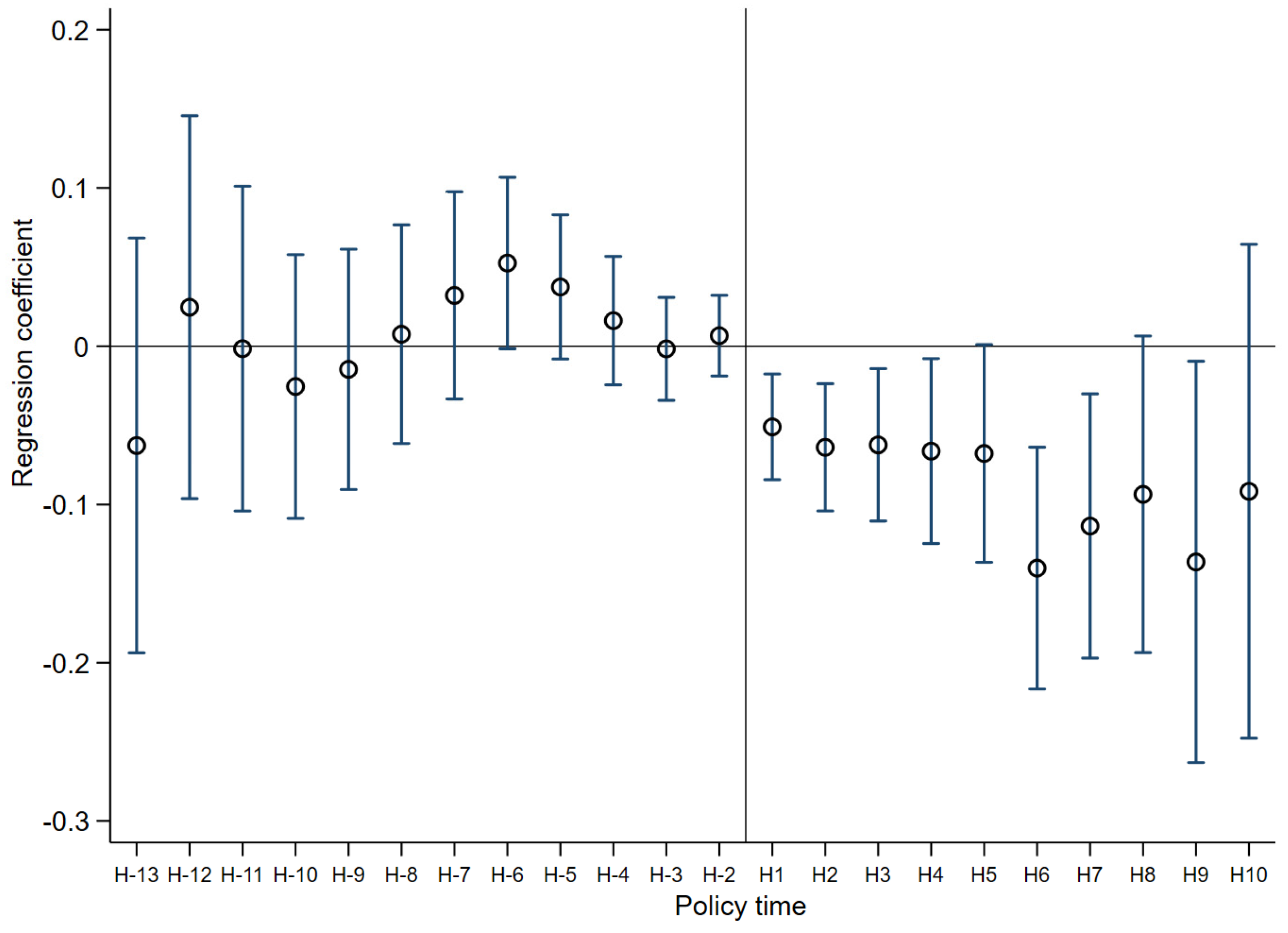
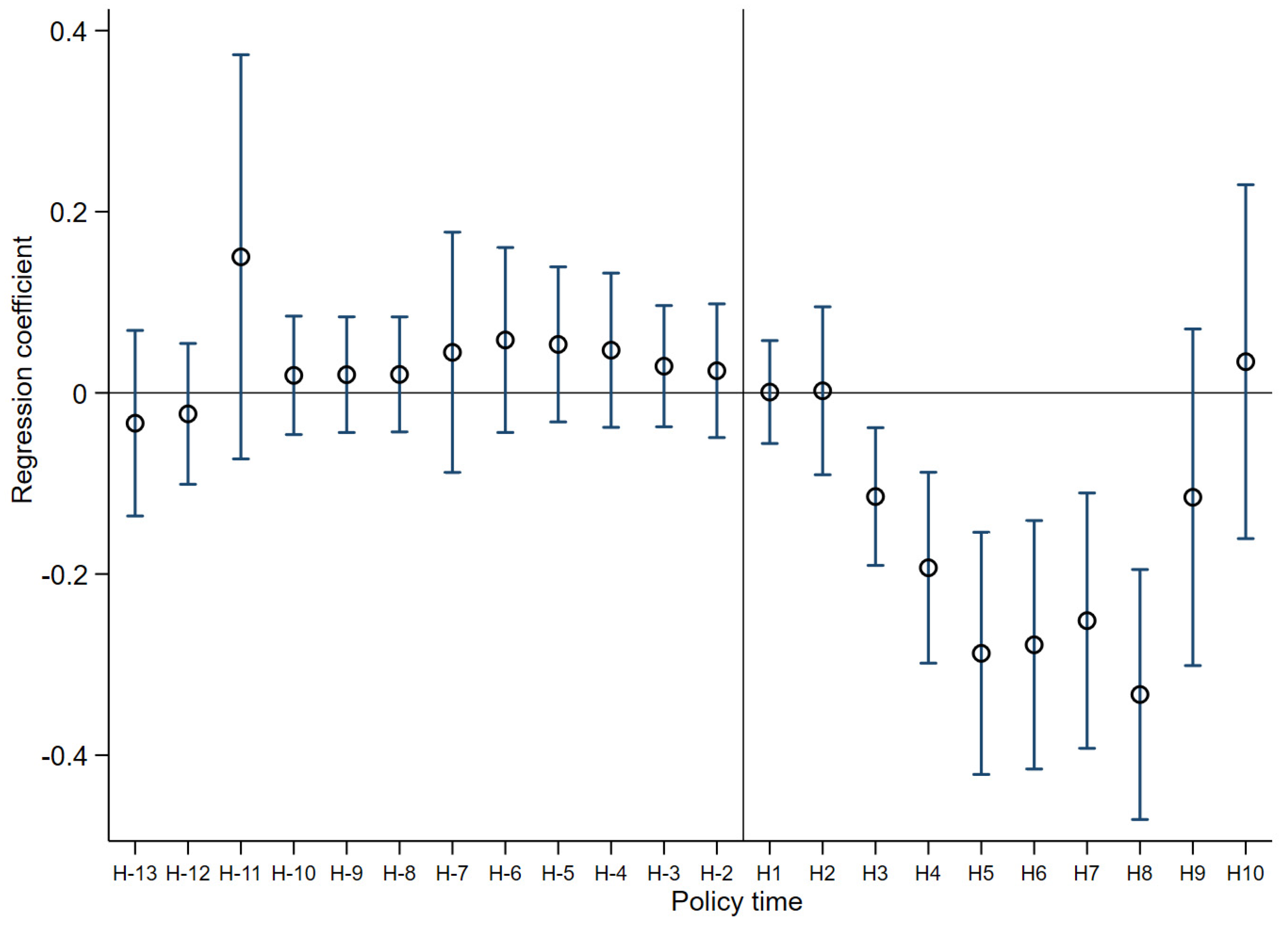
4.3.1. Parallel Trend Test

According to the basic assumption of the DID model, cities with and without HSR should have the same characteristics and development trends before HSR opening. Therefore, we construct the regression model shown in Equation (5) to test the parallel trend of the sample.

$$Y_{i,t}=\alpha +{\beta }_k{\displaystyle \sum _{k=1}^{13}H\_k_{i,t}}+{\beta }_l{\displaystyle \sum _{l=1}^{10}H{l}_{i,t}}+\varphi X_{i,t}+{\lambda }_t+{\delta }_i+{\epsilon }_{i,t}$$

(5)

In Equation (5), Y represents the urban financial agglomeration variable, which is AGGE or AGGD. H_1 to H_13 are dummy variables referring to 1 to 13 years before the opening of HSR, and the variables $H\_k$ take the value of 1 in the kth year before the HSR opening and 0 in the other years. H1 to H10 are dummy variables referring to 1 to 10 years after the opening of the HSR, and variables Hl also take a value of 0 or 1. X denotes the control variables, which are constructed in the same way as above. Figure 2 and Figure 3 show the confidence intervals of the $H\_k$ and $Hl$ coefficients β in the regressions. As shown in the figures, none of the regression coefficients of the HSR advance term ($H\_k$) are significantly different from 0, indicating that there are no significant differences between the cities with and the cities without HSR before the HSR opening. In other words, the DID model satisfies the parallel trend assumption. Meanwhile, one year after the HSR opening, a difference between the two groups of cities gradually emerges and expands over time, reflecting the persistence of HSR’s impact.

4.3.2. Propensity Score Matching Test

To reduce the interference of sample selectivity bias, we use the propensity score matching (PSM) method, which means that the control group is reconstructed by estimating the propensity score through a logit model and performing kernel matching based on the score. Regressions are conducted based on PSM, and

Table 5. PSM-DID regression results.

	AGGE	AGGD	AGGE	AGGD
	(13)	(14)	(15)	(16)
HSR	−0.0318 (−1.54)	−0.0416 ** (−2.00)
HSR_1			−0.0458 ** (−2.10)	−0.0347 ** (−2.11)
Control	yes	yes	yes	yes
Constant	1.0883 *** (3.93)	0.3086 (0.81)	1.0939 *** (3.95)	0.3043 (0.80)
City fixed effect	yes	yes	yes	yes
Year fixed effect	yes	yes	yes	yes
Observations	3550	3550	3550	3550

**, *** represent p-values less than 0.05, 0.01, respectively.

shows the regression results for the matched samples. The results show that the coefficient of HSR remains significantly negative, further validating H1 and reflecting the robustness of the aforementioned regression result.

4.3.3. Placebo Test

Table 5 verifies the robustness of the results obtained via PSM; however, this still cannot negate the influence of other unobservable factors. To further test the comparability of the treatment and control groups, a placebo test is conducted in this work to advance the opening time of HSR in each prefecture-level city by 1 to 3 years, and we re-run the DID regression. The results (as shown in

Table 6. Placebo test results.

	1 Year Advanced		2 Years Advanced		3 Years Advanced
	AGGE	AGGD	AGGE	AGGD	AGGE	AGGD
	(17)	(18)	(19)	(20)	(21)	(22)
HSR	−0.0327 (−1.59)	−0.0538 (−1.10)	−0.0244 (−1.26)	−0.0198 (−0.49)	−0.0289 (−1.48)	−0.0083 (−0.25)
Control	yes	yes	yes	yes	yes	yes
Constant	1.1103 *** (3.57)	1.0957 * (1.89)	0.9091 * (1.71)	−0.7680 (−1.45)	0.7808 (1.40)	−1.0255 * (−1.74)
City fixed effect	yes	yes	yes	yes	yes	yes
Year fixed effect	yes	yes	yes	yes	yes	yes
Observations	3679	3679	3396	3396	3113	3113

*, *** represent p-values less than 0.1, 0.01, respectively.

) show that the regression coefficients of HSR are not significant regardless of the advancement of 1, 2, or 3 years, indicating that unobservable factors do not significantly interfere with the regression.

4.3.4. Excluding Provincial Capital and National Central Cities

Since provincial capital (or national central) and non-capital (or non-national central) cities differ in various aspects, provincial capital and national central cities, as the political, economic, and cultural centers of regions, have more advantages compared with other cities and tend to be more likely to receive large amounts of policy and resource tilts. Whether a city becomes a provincial capital or national central city may affect the national planning of HSR construction in the region [3]. Therefore, to reduce the resulting estimation bias, we regress the sample again while excluding provincial capital and central cities. The results are shown in

Table 7. Regression results of non-provincial capital and non-central cities.

	AGGE	AGGD	AGGE	AGGD
	(23)	(24)	(25)	(26)
HSR	−0.0529 ** (−2.05)	−0.0780 ** (−1.98)
HSR_1			−0.0707 ** (−2.34)	−0.0934 ** (−2.34)
Control	yes	yes	yes	yes
Constant	0.8665 *** (2.99)	0.4748 (0.97)	0.8809 *** (3.07)	0.4872 (0.99)
City fixed effect	yes	yes	yes	yes
Year fixed effect	yes	yes	yes	yes
Observations	3542	3542	3542	3542

**, *** represent p-values less than 0.05, 0.01, respectively.

. Columns (23)–(26) show that the coefficients of the variables HSR and HSR_1 are both significantly negative at the 5% level. HSR reduces the financial agglomeration of non-provincial capital and non-central cities, and its effect is stronger after a one-period lag.

5. Mechanisms, Heterogeneity, and Spatial Effect

Based on the regression results, we further analyze the influencing mechanisms, heterogeneity, and spatial effect of HSR.

5.1. Mechanism Analysis

5.1.1. Regional Innovation

When the innovative capacity is poor, a large amount of capital will be concentrated within a few powerful innovation cities (in China, such as Beijing, Shanghai, and Shenzhen), and the massive funds beyond cities’ demands cannot be absorbed, thus causing a pile-up. HSR enhances labor mobility and increases the frequency of face-to-face communication. Communication and exchange help to promote interregional information sharing and alleviate regional information asymmetry. Knowledge and technology are diffused through the transmission of “soft information”, giving impetus to regional innovation [31]. By promoting innovation, HSR generates new, innovative products and accelerates capital flows, which in turn changes the urban financial structure. In this study, the number of granted invention patents in prefecture-level cities is used to measure the level of urban innovation, and a mediation effect analysis is conducted to test the impact of HSR on urban financial agglomeration through promoting regional innovation. Considering the large differences between different classifications of patents, we refer to the treatment of patent indicators described by Hall et al. (2001), which standardizes the indicator using the IPC subclass of the invention patent according to Equation (6) (j represents the jth invention patent granted to city i in year t) [53]. The treated innovation indicator (PAT) is included in the regression, and the results are shown in

Table 8. Mediating effect of regional innovation.

	PAT	AGGE	AGGD	PAT	AGGE	AGGD
	(1)	(2)	(3)	(4)	(5)	(6)
PAT		−0.0022 *** (−5.11)	−0.0049 ** (−2.46)		−0.0022 *** (−5.09)	−0.0048 ** (−2.44)
HSR	14.1949 *** (6.70)	−0.0279 (−1.26)	0.0092 (0.37)
HSR_1				16.4457 *** (6.35)	−0.0397 (−1.59)	−0.0078 (−0.29)
Control	yes	yes	yes	yes	yes	yes
Constant	−112.1802 ** (−2.20)	0.9462 *** (3.01)	0.8896 ** (1.98)	−112.8118 ** (−2.21)	0.9547 *** (3.05)	0.9023 ** (2.00)
City fixed effect	yes	yes	yes	yes	yes	yes
Year fixed effect	yes	yes	yes	yes	yes	yes
Observations	3880	3880	3880	3880	3880	3880

**, *** represent p-values less than 0.05, 0.01, respectively.

.

$$PA{T}_{i,t}={\displaystyle \sum _{j=1}^n\left(j/\begin{array}{l}\mathrm{Average}\mathrm{number}\mathrm{of}\mathrm{cities}\prime \mathrm{invention}\mathrm{patents}\\ \mathrm{in}\mathrm{the}\mathrm{same}\mathrm{IPC}\mathrm{subclass}\mathrm{as}j\mathrm{in}\mathrm{year}t\end{array}\right)}$$

(6)

As shown in Table 8, the variables HSR and HSR_1 in columns (1) and (4) are both significantly positive at the 1% level, indicating that HSR promotes urban innovation. Combining columns (2)–(3) and (5)–(6), we can find that urban innovation is significantly and negatively correlated with financial agglomeration, and HSR reduces the average degree of financial agglomeration in cities by promoting innovation, i.e., H2a is verified. HSR enhances the inter-regional flow of resources and provides cities with a large number of innovative factors. The spillover effect is gradually enhanced along with the improvement in the urban innovation capacity. Related studies show that the more developed the transportation facilities are, the greater the scope of the knowledge spillover. Meanwhile, knowledge spillover plays an important role in changing urban financial activities [27]. To further verify that the knowledge spillover effect of urban innovation promotes financial diffusion and reduces urban financial agglomeration, we replace the innovation indicator with the number of forward citations of invention patents in prefecture-level cities for measurement (cited). The forward citation counts (cited) of urban patents reflect both the innovation quantity and innovation quality, and a higher forward citation count indicates stronger innovation capabilities. Moreover, cited reflects the intensity of the knowledge spillover from innovation, and a higher value indicates that urban knowledge and technology are more frequently learned and imitated, i.e., a stronger spillover effect. Similarly, we also standardize the patent forward citation indicator (cited), and the weight is the inverse of the average of the cities’ invention patent forward citation counts in the same IPC subclass in year t. The regression results are shown in

Table 9. Mediating effect of regional innovation.

	cited	AGGE	AGGD	cited	AGGE	AGGD
	(7)	(8)	(9)	(10)	(11)	(12)
cited		−0.0023 *** (−4.61)	−0.0054 ** (−2.53)		−0.0023 *** (−4.61)	−0.0053 ** (−2.50)
HSR	13.4488 *** (6.60)	−0.0282 (−1.31)	0.0122 (0.50)
HSR_1				16.1011 *** (6.31)	−0.0387 (−1.62)	−0.0013 (−0.05)
Control	yes	yes	yes	yes	yes	yes
Constant	−111.0551 ** (−2.19)	0.9372 *** (2.95)	0.8398 * (1.89)	−111.9082 ** (−2.21)	0.9450 *** (2.99)	0.8500 * (1.90)
City fixed effect	yes	yes	yes	yes	yes	yes
Year fixed effect	yes	yes	yes	yes	yes	yes
Observations	3880	3880	3880	3880	3880	3880

*, **, *** represent p-values less than 0.1, 0.05, 0.01, respectively.

.

The results in Table 9 remain consistent with those in Table 8. HSR increases the number of urban patent forward citations, which reflects the innovation knowledge spillover, and the financial diffusion effect is subsequently strengthened, which in turn reduces urban financial agglomeration. The regression results in Table 9 also reflect the mediating effect of regional innovation, further confirming H2a.

5.1.2. Industrial Structure

The improvement of the transportation infrastructure can change the regional industrial structure [27]. The improved factor mobility and resource integration capacity facilitated by HSR can promote regional structure optimization and industrial structure upgrading [42]. As a result, the upgrading of the industrial structure will inevitably reshape the financial structure [43]. This includes the reallocation of financial resources in different regions, adjustments to the financial pattern, and subsequent changes to urban financial agglomeration. Hence, we use the share of the tertiary industry in the GDP of each prefecture-level city to measure the urban industrial structure ($t\_ind$) and conduct a mediating effect analysis. The regression results are shown in

Table 10. Mediating effect of industrial structure.

	t_ind	AGGE	AGGD	t_ind	AGGE	AGGD
	(7)	(8)	(9)	(10)	(11)	(12)
t_ind		−0.0028 * (−1.77)	−0.0055 * (−1.89)		−0.0027 * (−1.74)	−0.0054 * (−1.87)
HSR	0.7617 ** (2.03)	−0.0559 ** (−2.46)	−0.0564 (−1.53)
HSR_1				0.7042 * (1.85)	−0.0733 *** (−2.82)	−0.0828 ** (−2.09)
Control	yes	yes	yes	yes	yes	yes
Constant	90.2044 *** (10.29)	1.4040 *** (3.54)	1.8060 *** (2.60)	90.2536 *** (10.30)	1.4103 *** (3.57)	1.8145 *** (2.62)
City fixed effect	yes	yes	yes	yes	yes	yes
Year fixed effect	yes	yes	yes	yes	yes	yes
Observations	3952	3952	3952	3952	3952	3952

*, **, *** represent p-values less than 0.1, 0.05, 0.01, respectively.

.

Columns (7) and (10) indicate that HSR promotes the upgrading of the urban industrial structure. As an efficient mode of passenger transportation, HSR offers increased convenience and can influence the development of the service industry [31]. The expansion of the service industry extends the reach of cities, while its high mobility characteristics provide a channel for the dissemination of financial resources. This supports H2b, indicating that HSR reduces urban financial agglomeration by promoting the upgrading of the industrial structure. HSR also accelerates the division of labor and specialization among regions, allowing cities to upgrade their industrial structures based on their comparative advantages. In this context, firms can increase their off-site investments and the financial distribution becomes more rational [50], enabling the more efficient allocation of funds on a larger scale and strengthening the financial spillover effect.

5.2. HSR Intensity Analysis

The basic model (Equations (3) and (4)) examines the impact of HSR on urban financial agglomeration by constructing a dummy variable regarding whether HSR opens (HSR takes the value of 0 or 1). However, this measure ignores the differences in the intensity of HSR opening in different cities. Here, the number of HSR lines with stations established in the city is used to measure the urban HSR intensity. In other words, the core explanatory variable, HSR, in the basic regression model is replaced with the HSR intensity variable ($HSRQ$), and the control variables remain unchanged. Moreover, as a comparison, we treat the HSR intensity variable with a one-period lag ($HSRQ\_1$). As shown in

Table 11. HSR intensity regression results.

	AGGE	AGGD	AGGE	AGGD
	(17)	(18)	(19)	(20)
HSRQ	−0.0458 *** (−3.48)	−0.0930 *** (−3.26)
HSRQ_1			−0.0507 *** (−3.66)	−0.1090 *** (−3.30)
Control	yes	yes	yes	yes
Constant	1.0684 *** (3.18)	1.1057 ** (2.34)	1.0604 *** (3.17)	1.0757 ** (2.31)
City fixed effect	yes	yes	yes	yes
Year fixed effect	yes	yes	yes	yes
Observations	3962	3962	3962	3962

**, *** represent p-values less than 0.05, 0.01, respectively.

, after the re-regressions, the coefficients of the core explanatory variables ($HSRQ$ or $HSRQ\_1$) are similar to those in Table 2, and they are significantly negative at the 1% level. This indicates that an increase in HSR access lines also reduces urban financial agglomeration, further reflecting the stronger financial diffusion effect of HSR. This effect can be constantly enhanced as the HSR network becomes denser and more intricate.

5.3. Heterogeneity Analysis

HSR breaks the existing boundaries of cities, thus changing the urban pattern. As a type of transportation infrastructure with network properties, it inherently generates two both siphon and diffusion effects [29]. In relatively economically developed regions, the siphon effect of HSR leads to an increase in urban agglomeration and the diffusion effect leads to a decrease, while the opposite occurs in less economically developed regions. The relative magnitude of the two effects also varies across regions [29]. Therefore, to measure the regional heterogeneity of HSR’s impact, we divide the sample cities into three regions: eastern, middle, and western. The interaction terms ($mHSR$ and $wHSR$) between HSR and the dummy variables of the middle and western regions are further included in the regressions, as shown in Equations (7) and (8). Here, ${\beta }_1$ represents the effect of HSR on urban financial agglomeration in the eastern region, while ${\beta }_1+{\beta }_2$ and ${\beta }_1+{\beta }_3$ represent the effect of HSR in the middle and western regions, respectively. If the financial diffusion effect generated by HSR is greater than the siphon effect, the financial factors should generally show a tendency to shift from the developed eastern region to the middle and western regions. The regression results are shown in

Table 12. Heterogeneity regression results.

	AGGE	AGGD	AGGE	AGGD
	(21)	(22)	(23)	(24)
HSR	−0.1213 *** (−3.18)	−0.2290 ** (−2.52)
HSR_1			−0.1361 *** (−3.10)	−0.2561 *** (−2.86)
mHSR	0.1246 *** (2.68)	0.2638 *** (2.62)
mHSR_1			0.1268 ** (2.54)	0.2884 *** (2.90)
wHSR	0.0767 (1.49)	0.3387 *** (3.32)
wHSR_1			0.0744 (1.32)	0.3369 *** (3.39)
Control	yes	yes	yes	yes
Constant	1.3643 *** (4.19)	1.8172 *** (3.05)	1.3683 *** (4.26)	1.8273 *** (3.08)
City fixed effect	yes	yes	yes	yes
Year fixed effect	yes	yes	yes	yes
Observations	3962	3962	3962	3962

**, *** represent p-values less than 0.05, 0.01, respectively.

.

$$AGG{E}_{i,t}=\alpha +{\beta }_{1}HS{R}_{i,t}+{\beta }_{2}mHS{R}_{i,t}+{\beta }_{3}wHS{R}_{i,t}+\varphi X_{i,t}+{\lambda }_t+{\delta }_i+{\epsilon }_{i,t}$$

(7)

$$AGG{D}_{i,t}=\alpha +{\beta }_{1}HS{R}_{i,t}+{\beta }_{2}mHS{R}_{i,t}+{\beta }_{3}wHS{R}_{i,t}+\varphi X_{i,t}+{\lambda }_t+{\delta }_i+{\epsilon }_{i,t}$$

(8)

The results show that ${\beta }_1$ is significantly negative in all regressions, indicating that the opening of HSR reduces financial agglomeration in the eastern region. Compared to the financial siphon effect, the eastern region is affected most strongly by the financial diffusion effect. This is due to the relatively developed economy and higher level of urban financial development, as well as the denser HSR network in the eastern region. The opening of HSR aggravates the spillover of financial resources from the region to the outside, and its convenience and improved access to information cause financial activities and financial transactions to occur on a larger scale and gradually extend to the middle, western, and even other non-prefecture-level cities, finally causing a decrease in urban financial agglomeration. In addition, the coefficients of ${\beta }_2$ and ${\beta }_3$ in the regression are positive and more significant. Combined with ${\beta }_1$, they show that the negative effect of HSR on financial agglomeration in the middle and western regions is not strong compared to that in the eastern region, and it even shows a somewhat promotional effect. In this context, it may benefit from the influence of financial spillover from the eastern region. By shortening the spatiotemporal distance between the middle and western regions and the eastern region, HSR promotes the transfer of financial resources, which further verifies the dominant financial diffusion effect.

5.4. Spatial Effect Analysis

5.4.1. Spatial Econometric Model

According to economic geography, the shorter the distance, the stronger the interactions between regions. The opening of HSR accelerates the flow of people, logistics, information, and capital between regions [4,5,6,11,12], thus intensifying the mutual influence of financial agglomeration in neighboring regions [14]. Since there may be spatial spillover effects of financial agglomeration and transportation infrastructure construction [27], we construct different spatial weight matrices and further take geographic factors into account to explore the spatial effects of HSR on urban financial agglomeration. In particular, the spatial Durbin model (SDM) is constructed, as shown in Equations (9) and (10).

$$AGG{E}_{i,t}=\alpha +\rho W\ast AGG{E}_{\mathrm{i},t}+\beta HS{R}_{i,t}+\theta W\ast HS{R}_{i,t}+\varphi X_{i,t}+{\lambda }_t+{\delta }_i+{\epsilon }_{i,t}$$

(9)

$$AGG{D}_{i,t}=\alpha +\rho W\ast AGG{D}_{\mathrm{i},t}+\beta HS{R}_{i,t}+\theta W\ast HS{R}_{i,t}+\varphi X_{i,t}+{\lambda }_t+{\delta }_i+{\epsilon }_{i,t}$$

(10)

where W is the spatial weight matrix. We construct a 0–1 adjacency matrix, geographic distance matrix, economic distance matrix, and nested matrix, which consider both geographic and economic factors for analysis, based on the latitude and longitude information of each prefecture-level city. The other variables remain unchanged. The specific details of the matrices ($W$) constructed are as follows.

(1)

0–1 adjacency matrix ($W_1$): This can concisely and intuitively represent the bordering positions of prefecture-level cities in geospatial terms. If cities i and j are adjacent, $W_{ij}=1$; otherwise, $W_{ij}=0$.

(2)

Geographic distance matrix ($W_2$): The construction of the adjacency matrix is intuitive, but it ignores the influence of distance differences among non-adjacent cities. Therefore, we also construct a geographic distance matrix, reflecting the degree of proximity between cities, for regression. Specifically, the Euclidean distance ($d_{ij}$) between city i and city j is calculated, and then the matrix $W_2$ is constructed using the reciprocal of the square of this distance, which is

$$W_{ij}=\left\{\begin{array}{ll}1/d_{ij}^2\hfill & i\ne j\hfill \\ 0\hfill & i=j\hfill \end{array}\right.$$

(3)

Economic distance matrix ($W_3$): The geographic distance matrix reflects the differences in the geographical locations of cities. However, the spatial effects are not only related to geographical factors but may also be influenced by socioeconomic factors. We take the GDP per capita (e) of city i and city j as a measure and construct an economic distance matrix by using the reciprocal of the absolute value of the difference between them, which is

$$W_{ij}=\left\{\begin{array}{ll}1/|e_i-e_j|\hfill & i\ne j\hfill \\ 0\hfill & i=j\hfill \end{array}\right.$$

(4)

Nested matrix ($W_4$): In order to examine the integrated effects of geographic and economic factors, we further construct a spatial nested matrix containing both factors for analysis. The equation is $W_{\mathrm{ij}}=W_d\times \mathrm{diag}\left({\overline{X}}_{\mathrm{l}}/\overline{X},{\overline{X}}_2/\overline{X},\cdots ,{\overline{X}}_n/\overline{X}\right)$. Here, $W_d$ is the reciprocal distance matrix. The ${\overline{X}}_i$ in diagonal elements represents the average value of the GDP per capita in city i. $\overline{X}$ represents the average GDP per capita of all cities in the sample interval.

5.4.2. Spatial Correlation Test

The global Moran’s I index (Moran’s I) is constructed to measure the spatial correlations of different cities, as shown in Equation (11):

$$Moran\prime s I=\frac{{\displaystyle \sum _{i=1}^n{\displaystyle \sum _{j=1}^n{W}_{ij}(Y_i-\overline{Y})(Y_j-\overline{Y})}}}{S^2{\displaystyle \sum _{i=1}^n{\displaystyle \sum _{j=1}^n{W}_{ij}}}}$$

(11)

where $S^2=\frac{1}{n}{\displaystyle \sum _{i=1}^n(Y_i}-\overline{Y}{)}^2$ is the sample variance. $W_{ij}$ represents the four spatial weight matrices. The Moran’s I takes values in the range of −1 to 1. It is positively spatially correlated when it is greater than 0, and it is negatively spatially correlated when it is less than 0. A larger absolute value of the index indicates a stronger correlation, and a value of 0 indicates that there is no spatial correlation.

Based on the four spatial weight matrices, we measure the Moran’s I of HSR and financial agglomeration in the prefecture-level cities, and the results are shown in

Table A1. Spatial correlation test results.

	${\mathit{W}}_1$			${\mathit{W}}_2$			${\mathit{W}}_3$			${\mathit{W}}_4$
	AGGE	AGGD	HSR	AGGE	AGGD	HSR	AGGE	AGGD	HSR	AGGE	AGGD	HSR
2005	0.108 *** (3.167)	0.376 *** (12.203)		0.047 *** (2.678)	0.218 *** (13.342)		0.120 *** (3.359)	0.372 *** (11.571)		0.011 ** (2.552)	0.064 *** (13.629)
2006	0.133 *** (3.872)	0.505 *** (15.915)		0.058 *** (3.297)	0.375 *** (22.189)		0.123 *** (3.440)	0.504 *** (15.196)		0.013 *** (3.026)	0.095 *** (19.401)
2007	0.133 *** (3.863)	0.530 *** (16.396)		0.058 *** (3.288)	0.389 *** (22.606)		0.131 *** (3.663)	0.533 *** (15.797)		0.012 *** (2.882)	0.100 *** (19.951)
2008	0.143 *** (4.167)	0.527 *** (16.216)	0.326 *** (9.798)	0.056 *** (3.143)	0.385 *** (22.220)	0.174 *** (9.858)	0.136 *** (3.803)	0.534 *** (15.743)	0.147 *** (4.282)	0.014 *** (3.136)	0.099 *** (19.662)	0.067 *** (13.172)
2009	0.144 *** (4.176)	0.513 *** (15.568)	0.254 *** (7.395)	0.063 *** (3.526)	0.367 *** (20.942)	0.128 *** (7.064)	0.139 *** (3.866)	0.539 *** (15.644)	0.169 *** (4.741)	0.015 *** (3.308)	0.095 *** (18.814)	0.065 *** (12.472)
2010	0.158 *** (4.585)	0.315 *** (9.553)	0.245 *** (7.056)	0.067 *** (3.732)	0.207 *** (11.844)	0.111 *** (6.088)	0.134 *** (3.742)	0.394 *** (11.415)	0.146 *** (4.072)	0.014 *** (3.120)	0.061 *** (12.289)	0.035 *** (6.905)
2011	0.139 *** (4.064)	0.192 *** (5.642)	0.244 *** (6.998)	0.059 *** (3.363)	0.097 *** (5.451)	0.161 *** (8.726)	0.088 ** (2.499)	0.267 *** (7.477)	0.292 *** (7.978)	0.010 ** (2.450)	0.035 *** (7.136)	0.055 *** (10.584)
2012	0.130 *** (3.807)	0.521 *** (15.620)	0.273 *** (7.811)	0.057 *** (3.216)	0.367 *** (20.685)	0.178 *** (9.580)	0.077 ** (2.188)	0.553 *** (15.879)	0.328 *** (8.950)	0.009 ** (2.208)	0.094 *** (18.401)	0.059 *** (11.265)
2013	0.220 *** (6.311)	0.528 *** (15.724)	0.319 *** (9.077)	0.106 *** (5.788)	0.367 *** (20.556)	0.217 *** (11.635)	0.149 *** (4.128)	0.562 *** (16.034)	0.302 *** (8.242)	0.028 *** (5.645)	0.095 *** (18.380)	0.072 *** (13.669)
2014	0.220 *** (6.315)	0.536 *** (15.917)	0.325 *** (9.264)	0.102 *** (5.576)	0.370 *** (20.653)	0.203 *** (10.894)	0.169 *** (4.679)	0.568 *** (16.169)	0.255 *** (6.959)	0.024 *** (4.972)	0.095 *** (18.488)	0.056 *** (10.724)
2015	0.217 *** (6.253)	0.524 *** (15.343)	0.284 *** (8.083)	0.103 *** (5.642)	0.353 *** (19.429)	0.184 *** (9.867)	0.157 *** (4.353)	0.587 *** (16.445)	0.263 *** (7.182)	0.024 *** (5.071)	0.093 *** (17.792)	0.056 *** (10.689)
2016	0.216 *** (6.224)	0.523 *** (15.270)	0.281 *** (8.021)	0.105 *** (5.747)	0.349 *** (19.130)	0.187 *** (10.047)	0.172 *** (4.758)	0.586 *** (16.364)	0.245 *** (6.701)	0.026 *** (5.300)	0.092 *** (17.680)	0.061 *** (11.689)
2017	0.235 *** (6.752)	0.474 *** (13.761)	0.229 *** (6.541)	0.118 *** (6.468)	0.311 *** (16.993)	0.164 *** (8.868)	0.180 *** (4.975)	0.546 *** (15.171)	0.225 *** (6.161)	0.035 *** (7.011)	0.083 *** (15.943)	0.055 *** (10.585)
2018	0.216 *** (6.240)	0.383 *** (11.227)	0.218 *** (6.235)	0.114 *** (6.259)	0.256 *** (14.132)	0.156 *** (8.449)	0.169 *** (4.690)	0.519 *** (14.526)	0.202 *** (5.557)	0.037 *** (7.327)	0.064 *** (12.449)	0.048 *** (9.282)

**, *** represent p-values less than 0.05, 0.01, respectively.

in Appendix A. Most values are significantly positive at the 5% level, indicating a significant positive spatial correlation.

5.4.3. Spatial Regression

Table A2. LM test results.

	${\mathit{W}}_1$		${\mathit{W}}_2$		${\mathit{W}}_3$		${\mathit{W}}_4$
	AGGE	AGGD	AGGE	AGGD	AGGE	AGGD	AGGE	AGGD
Spatial error: LM test	2008.231 ***	983.925 ***	1223.831 ***	394.808 ***	17.172 ***	3.197 *	4115.277 ***	2031.174 ***
Spatial error: robust LM test	293.155 ***	322.823 ***	1062.504 ***	249.254 ***	15.202 ***	0.805	3928.442 ***	1828.472 ***
spatial lag: LM test	1728.932 ***	784.664 ***	162.945 ***	185.515 ***	1.975	3.492 *	186.865 ***	239.668 ***
spatial lag: robust LM test	13.856 ***	123.562 ***	1.617	39.961 ***	0.005	1.100	0.030	36.966 ***
Spatial lag: LR test	12.98 ***	81.01 ***	26.24 ***	82.30 ***	30.33 ***	90.50 ***	38.79 ***	64.81 ***
Spatial error: LR test	1370.82 ***	1378.96 ***	1350.63 ***	1339.64 ***	1451.08 ***	1330.21 ***	1331.63 ***	1392.48 ***
Hausman ${\chi }^2$	65.55 ***	43.23 ***	70.88 ***	34.38 ***	55.78 ***	43.09 ***	78.25 ***	38.46 ***

*, *** represent p-values less than 0.1, 0.01, respectively.

in Appendix B. The LM tests of different matrices are mostly significant, reflecting the necessity of constructing a spatial model. The following LR test rejects the possible degradation of SDM and confirms the reasonableness of Equations (9) and (10). According to the Hausman test, the spatial regression is also controlled for city and year two-way fixed effects and the total effect is further decomposed via partial differentiation. The results are shown in

Table 13. Spatial regression results.

	${\mathit{W}}_1$		${\mathit{W}}_2$		${\mathit{W}}_3$		${\mathit{W}}_4$
	AGGE	AGGD	AGGE	AGGD	AGGE	AGGD	AGGE	AGGD
	(1)	(2)	(3)	(4)	(5)	(6)	(7)	(8)
W*AGGE/W*AGGD	0.3145 *** (9.04)	0.3755 *** (8.87)	0.5205 *** (7.36)	0.6115 *** (10.49)	0.3012 *** (5.53)	0.4884 *** (10.41)	0.8009 *** (23.15)	0.8564 *** (32.64)
HSR	−0.0454 * (−1.90)	0.0206 (0.70)	−0.0274 (−1.16)	0.0367 (1.21)	−0.0356 (−1.60)	0.0101 (0.34)	−0.0432 * (−1.89)	−0.0110 (−0.33)
W*HSR	−0.0624 * (−1.73)	−0.2820 *** (−2.85)	−0.1019 ** (−2.36)	−0.3266 *** (−2.68)	−0.0955 ** (−2.46)	−0.2882 *** (−3.05)	−0.1277 *** (−2.69)	−0.2992 ** (−2.41)
Control	yes	yes	yes	yes	yes	yes	yes	yes
Constant	0.8360 *** (4.95)	−0.9280 *** (−3.14)	0.5816 *** (2.94)	−1.1284 *** (−3.49)	0.8583 *** (4.52)	−0.9238 *** (−3.89)	0.2083 (1.26)	−1.2093 *** (−3.38)
City fixed effect	yes	yes	yes	yes	yes	yes	yes	yes
Year fixed effect	yes	yes	yes	yes	yes	yes	yes	yes
Observations	3962	3962	3962	3962	3962	3962	3962	3962
Direct: HSR	−0.0492 ** (−2.08)	0.0002 (0.01)	−0.0308 (−1.30)	0.0237 (0.74)	−0.0411 * (−1.84)	−0.0203 (−0.55)	−0.0454 * (−1.95)	−0.0176 (−0.50)
Indirect: HSR	−0.1069 ** (−2.32)	−0.4245 ** (−2.55)	−0.2478 ** (−2.51)	−0.7968 ** (−2.11)	−0.1449 *** (−3.01)	−0.5313 *** (−2.69)	−0.8463 *** (−2.72)	−2.1927 ** (−2.13)
Total: HSR	−0.1561 *** (−3.66)	−0.4242 ** (−2.32)	−0.2786 *** (−2.88)	−0.7731 ** (−2.00)	−0.1860 *** (−3.99)	−0.5516 ** (−2.49)	−0.8917 *** (−2.89)	−2.2104 ** (−2.11)

*, **, *** represent p-values less than 0.1, 0.05, 0.01, respectively.

.

In Table 13, the coefficients of $W^{*}AGGE$ and $W^{*}AGGD$ are both significantly positive at the 1% level, indicating that urban financial agglomeration exhibits a positive spatial correlation regardless of which spatial matrix is used for regression. This is consistent with the results of the aforementioned Moran’s I test, indicating that urban financial agglomeration has a spatial dependence of high–high or low–low agglomeration within a certain range, i.e., the deepening of local financial agglomeration has a positive impact on financial agglomeration in neighboring (geographical or economic) areas. This effect continues to weaken with increasing geographical distance or economic disparity. Meanwhile, the regression coefficients of $W^{*}HSR$ are all significantly negative, indicating that the opening of HSR in a neighboring city has a negative effect on the local financial agglomeration. In terms of the effect decomposition, the direct and indirect effects of HSR on urban financial agglomeration are significantly negative in general. On the one hand, urban HSR opening reduces local financial agglomeration and will create a feedback effect via a decline in financial agglomeration in neighboring areas. On the other hand, the opening of HSR in neighboring areas also leads to a decrease in local financial agglomeration, and this effect is more obvious than the direct effect.

These results may be attributed to the differences in the scope of the financial siphon and diffusion effects. According to the Moran’s I and the coefficients of the spatial lag term, we find that the closeness of urban financial agglomeration increases with the shortening of the geographical and economic distances, and it presents similar distribution characteristics within a certain range. On the one hand, after the opening of HSR, the inter-regional spatial and temporal barriers are broken, which results in a financial diffusion effect across a broader range. For geographically neighboring cities, the spatial and temporal compression effect of HSR is not obvious within neighboring cities due to their short spatial distances from each other, but it mainly generates a financial diffusion effect from cities within the neighboring range to cities outside this range. In economically neighboring cities, their similar development levels and agglomeration characteristics lead to similar effects of HSR. Due to the enhanced connectivity between cities within the neighboring range and cities outside this range, financial factors and knowledge can be transferred and spilled across the region through the HSR network, accelerating financial diffusion outward, which in turn leads to a decrease in financial agglomeration in HSR cities and their neighboring cities within a certain range. On the other hand, the financial diffusion effect needs to be realized through the HSR network. After a city opens HSR, the financial resources of its neighboring cities will be transferred to this HSR city, thus realizing diffusion via HSR. This process causes the HSR city to produce a financial siphon effect on its neighboring cities, which, to some extent, offsets its own financial diffusion to cities outside the neighboring range, causing the magnitude and significance of its direct effect to be reduced.

6. Conclusions

This study utilized panel data from 2005 to 2018 on 283 prefecture-level cities in China to construct a DID model that examines the impact of high-speed rail (HSR) on urban financial agglomeration. The findings indicate that HSR significantly decreases urban financial agglomeration. First, HSR promotes urban innovation and forms knowledge spillover, which leads to financial diffusion. Second, HSR contributes to industrial structure upgrading and prevents the over-concentration of financial agglomeration by adjusting the industrial structure. The heterogeneity analysis further shows that the financial diffusion generated by HSR mainly presents an east-to-west direction in China. Finally, the negative impact of HSR on urban financial agglomeration is further verified by constructing four different spatial weight matrices to conduct spatial regressions. We find that HSR widens the range of financial diffusion and its indirect effect on financial agglomeration is more pronounced compared to the direct effect.

HSR construction has a dual nature comprising both diffusion and siphon effects, presenting both opportunities and challenges. In view of these two aspects, cities should pursue staggered competition, leveraging their comparative advantages and forming complementary partnerships with larger cities. Local governments should also seize the opportunity of spatiotemporal compression created by HSR, making use of the overflow of knowledge, experience, and technology brought by HSR to stimulate innovative urban development and strengthen their technological innovation. By promoting high-quality innovation, they can allocate and use their capital effectively, avoiding the aggravation of financial bubbles while supporting the healthy expansion of the financial scale. In addition, local governments need to enhance the construction of financial infrastructure, establish systems for the introduction of financial talent, improve the relevant institutional mechanisms, shorten the matching time between talent and jobs, and ensure that the financial diffusion effect of HSR is fully utilized. Overall, cities in the “HSR era” should seize the opportunities provided and embrace the challenges, understand the essence of finance, and develop new modes or business types, such as inclusive finance, green finance, and technology finance, based on the local conditions. These measures are expected to enhance financial innovation, optimize the financial service structure, enhance the industrial support capabilities, and help the financial industry to achieve high-quality development.

Differing from the agglomeration trends of traditional industries or the labor force, this study reveals the diffusion effect of HSR on finance from the perspective of the financial industry. However, a limitation of this study is that it does not compare the impact of HSR on the financial industry and other industries, especially traditional industries. In addition, this study fails to prove the diffusion effect of the financial industry in the county or county-level city. These two aspects of analysis constitute possible directions for future research.

References

1. Zhang, X.L. Has Transport lnfrastructure Promoted Regional Economic Growth?—With an Analysis of the Spatial Spillover Effects of Transport lnfrastructure. Soc. Sci. China 2012, 34, 60–77+206. [Google Scholar]
2. Lu, J.; Song, J.T.; Liang, Y.S. The Simulation of Spatial Distribution Patterns of China’s HSR-economic Zones Based on the 2D Time-space Map. Acta Geogr. Sin. 2013, 68, 147–158. [Google Scholar]
3. Liu, Y.Z.; Li, Y. High-speed Rails and City Economic Growth in China. J. Financ. Res. 2017, 11, 18–33. [Google Scholar]
4. Hu, Y.; Deng, T.; Zhang, J. Can Commuting Facilitation Relieve Spatial Misallocation of Labor? Habitat Int. 2020, 106, 102136. [Google Scholar] [CrossRef]
5. Sun, P.Y.; Zhang, T.T.; Yao, S.J. Tariff Transmission, Domestic Transport Costs and Retail Prices. Econ. Res. J. 2019, 54, 135–149. [Google Scholar]
6. Zhang, X.; Wu, W.; Zhou, Z. Geographic Proximity, Information Flows and Corporate Innovation: Evidence from the High-Speed Rail Construction in China. Pac. Basin Financ. J. 2020, 61, 101342. [Google Scholar] [CrossRef]
7. Wang, X.; Zhu, Y.; Ren, X.; Gozgor, G. The impact of digital inclusive finance on the spatial convergence of the green total factor productivity in the Chinese cities. Appl. Econ. 2023, 55, 4871–4889. [Google Scholar] [CrossRef]
8. Du, Y.; Wang, Q.; Zhou, J. How does digital inclusive finance affect economic resilience: Evidence from 285 cities in China. Int. Rev. Financ. Anal. 2023, 88, 102709. [Google Scholar] [CrossRef]
9. Yue, H.; Zhou, Z.; Liu, H. How does green finance influence industrial green total factor productivity? Empirical research from China. Energy Rep. 2024, 11, 914–924. [Google Scholar] [CrossRef]
10. Fan, W.; Wang, F.; Liu, S.; Chen, T.; Bai, X.; Zhang, Y. How does financial and manufacturing co-agglomeration affect environmental pollution? Evidence from China. J. Environ. Manag. 2023, 325, 116544. [Google Scholar] [CrossRef]
11. Guan, C.; Hu, Q. Does high-speed railway impact urban logistics industry agglomeration? Empirical evidence from China’s prefecture-level cities. Socio-Econ. Plan. Sci. 2023, 87, 101557. [Google Scholar] [CrossRef]
12. Han, D.; Attipoe, S.G.; Han, D.; Cao, J. Does transportation infrastructure construction promote population agglomeration? Evidence from 1838 Chinese county-level administrative units. Cities 2023, 140, 104409. [Google Scholar] [CrossRef]
13. Chen, H.; Zhu, T.; Zhao, L. High-Speed Railway Opening, Industrial Symbiotic Agglomeration and Green Sustainable Development—Empirical Evidence from China. Sustainability 2024, 16, 2070. [Google Scholar] [CrossRef]
14. Kwilinski, A.; Lyulyov, O.; Pimonenko, T. Spillover Effects of Green Finance on Attaining Sustainable Development: Spatial Durbin Model. Computation 2023, 11, 199. [Google Scholar] [CrossRef]
15. Huang, C.; Han, Q.; Tan, X.; Hua, Y.; Shang, L. High-speed rail operations, the cross-regional mobility of highly skilled talent, and regional innovation—Evidence from the Yangtze River delta in China. Appl. Econ. 2024, 1–18. [Google Scholar] [CrossRef]
16. Wang, L.; Wu, Y.; Chen, Y.; Dai, Y. Distance produces the fear of loss: Customer geographic proximity and corporate cash holdings. Int. Rev. Financ. Anal. 2023, 87, 102572. [Google Scholar] [CrossRef]
17. Atack, J.; Bateman, F.; Haines, M. Did Railroads Induce or Follow Economic Growth? Urbanization and Population Growth in the American Midwest, 1850–1860. Soc. Sci. Hist. 2010, 34, 171–197. [Google Scholar] [CrossRef]
18. Vickerman, R. High-speed rail in Europe: Experience and Issues for Future Development. Ann. Reg. Sci. 1997, 31, 21–38. [Google Scholar] [CrossRef]
19. Chen, Z.; Haynes, K.E. Impact of high speed rail on housing values: An observation from the Beijing–Shanghai line. J. Transp. Geogr. 2015, 43, 91–100. [Google Scholar] [CrossRef]
20. Wang, Y.F.; Ni, P.F. Economic Growth Spillover and Spatial Optimization of High-speed Railway. China Ind. Econ. 2016, 2, 21–36. [Google Scholar]
21. Krugman, P. Increasing Returns and Economic-geography. J. Political Econ. 1991, 99, 483–499. [Google Scholar] [CrossRef]
22. Ran, W.; Rong, W. Exploring Financial Agglomeration and the Impact of Environmental Regulation on the Efficiency of the Green Economy: Fresh Evidence from 30 Regions in China. Sustainability 2023, 15, 7226. [Google Scholar] [CrossRef]
23. Iyare, S.; Moore, W. Financial Sector Development and Growth in Small Open Economies. Appl. Econ. 2011, 43, 1289–1297. [Google Scholar] [CrossRef]
24. Gordon, I.R. Quantitative Easing of an International Financial Centre: How Central London Came So Well Out of the Post-2007 Crisis. Camb. J. Reg. Econ. Soc. 2016, 9, 335–353. [Google Scholar] [CrossRef]
25. Nicolae, P.V. Theoretical and Practical Considerations on Financial Autonomy and Balance Local Budgets in Romania. Econ. Ser. 2015, 2, 231–238. [Google Scholar]
26. Ding, X.; Liu, X. Renewable Energy Development and Transportation Infrastructure Matters for Green Economic Growth? Empirical Evidence from China. Econ. Anal. Policy 2023, 79, 634–646. [Google Scholar] [CrossRef]
27. Wang, Z.L.; Lin, X.Y.; Gao, H.W. A Study on the Impact of Transportation Infrastructure on Financial Agglomeration: An Evidence Based on Railways and Highways. Macroeconomics 2020, 12, 47–61+120. [Google Scholar]
28. Laulajainen, R. Financial Geography: A Banker’s View; Taylor and Francis: Oxfordshire, UK, 2003. [Google Scholar]
29. Vickerman, R. High-speed rail and regional development: The case of intermediate stations. J. Transp. Geogr. 2015, 42, 157–165. [Google Scholar] [CrossRef]
30. Zhang, K.Z.; Tao, D.J. Economic Distribution Effects of Transportation Infrastructure: Evidence from the Opening of High Speed Rail. Econ. Perspect. 2016, 6, 62–73. [Google Scholar]
31. Qin, Y. ‘No county left behind?’ The Distributional Impact of High-Speed Rail Upgrades in China. J. Econ. Geogr. 2017, 17, 489–520. [Google Scholar] [CrossRef]
32. Behrens, K.; Lamorgese, A.R.; Ottaviano, G.I. Changes in Transport and Non-Transport Costs: Local vs Global Impacts in a Spatial Network. Reg. Sci. Urban Econ. 2007, 37, 625–648. [Google Scholar] [CrossRef]
33. Li, H.C.; Tjia, L.; Hu, S.X. Agglomeration and Equalization Effect of High Speed Railway on Cities in China. J. Quant. Tech. 2016, 33, 127–143. [Google Scholar]
34. Wang, Y.; Zhang, F. High-speed rail and distribution of economic activities: Evidence from prefecture-level cities in China. Res. Transp. Bus. Manag. 2023, 51, 101065. [Google Scholar] [CrossRef]
35. Chen, M.; Liu, X.; Xiong, X.; Wu, J. Has the opening of high-speed rail narrowed the inter-county economic gap? The perspective of China’s state-designated poor counties. Int. Rev. Econ. Financ. 2023, 88, 1–13. [Google Scholar] [CrossRef]
36. He, L.Y.; Liu, S. Impact of China Railway Express on Regional Resource Mismatch—Empirical Evidence from China. Sustainability 2023, 15, 8441. [Google Scholar] [CrossRef]
37. Zhao, J.; Huang, J.C.; Liu, F. China High-speed Railways and Stock Price Crash Risk. J. Manag. World 2018, 34, 157–168+192. [Google Scholar]
38. Zhou, W.T.; Yang, R.D.; Hou, X.S. High-speed Rail Network, Location Advantage and Regional Innovation. Econ. Rev. 2021, 4, 75–95. [Google Scholar]
39. Alexander, B.; Dijst, M. Professional Workers at Work: Importance of Work Activities for Electronic and Face-to-Face Communications in the Netherlands. Transportation 2012, 39, 919–940. [Google Scholar] [CrossRef]
40. Bian, Y.C.; Wu, L.H.; Bai, J.H. Does High-speed Rail Improve Regional Innovation in China? J. Financ. Res. 2019, 6, 132–149. [Google Scholar]
41. Zhu, Z.J.; Huang, X.H.; Wang, H. Does Traffic Infrastructure Promote Innovation? A Quasi-natural Experiment Based on the Expansion of the High-speed Railway Network in China. J. Financ. Res. 2019, 11, 153–169. [Google Scholar]
42. Zhang, J.B. Research on the Impact of Transportation Infrastructure Construction on Industrial Structure Transformation. J. Yunnan Univ. Financ. Econ. 2018, 34, 35–46. [Google Scholar]
43. Gong, Q.; Zhang, Y.L.; Lin, Y.F. Industrial Structure, Risk Feature and Optimal Financial Structure. Econ. Res. J. 2014, 49, 4–16. [Google Scholar]
44. Chen, F.; Shao, M.; Dai, J.; Chen, W. Can the opening of high-speed rail reduce environmental pollution? An empirical research based on difference-in-differences model. Clean Technol. Environ. Policy 2024, 1–13. [Google Scholar] [CrossRef]
45. Nie, L.; Zhang, Z. Is high-speed rail heading towards a low-carbon industry? Evidence from a quasi-natural experiment in China. Resour. Energy Econ. 2023, 72, 101355. [Google Scholar] [CrossRef]
46. Sun, W.Z.; Niu, D.X.; Wan, G.H. Transportation Infrastructure and Industrial Structure Upgrading: Evidence from China’s High-speed Railway. J. Manag. World 2022, 38, 19–34+58+35–41. [Google Scholar]
47. Hu, M.; Xu, J. How Does High-Speed Rail Impact the Industry Structure? Evidence from China. Urban Rail. Transit. 2022, 8, 296–317. [Google Scholar] [CrossRef]
48. Brezdeń, P.; Sikorski, D. Processes of Spatial Concentration and Specialisation of Industry by the Intensity of R & D Work in the Lower Silesian Voivodeship (Poland). Quaest. Geogr. 2023, 42, 19–36. [Google Scholar]
49. Chen, C.-L.; Vickerman, R. Can transport infrastructure change regions’ economic fortunes? Some evidence from Europe and China. Reg. Stud. 2017, 51, 144–160. [Google Scholar] [CrossRef]
50. Ma, G.R.; Cheng, X.M.; Yang, E.Y. How Does Transportation Infrastructure Affect Capital Flows—A Study from High-speed Rail and Cross-region Investment of Listed Companies. China Ind. Econ. 2020, 6, 5–23. [Google Scholar]
51. Dong, X.; Zheng, S.; Kahn, M.E. The role of transportation speed in facilitating high skilled teamwork across cities. J. Urban Econ. 2020, 115, 103212. [Google Scholar] [CrossRef]
52. Niu, D.; Sun, W.; Zheng, S. Travel costs, trade, and market segmentation: Evidence from China’s high-speed railway. Pap. Reg. Sci. 2020, 99, 1799–1826. [Google Scholar] [CrossRef]
53. Hall, B.H.; Jaffe, A.B.; Trajtenberg, M. The NBER Patent Citation Data File: Lessons, Insights and Methodological Tools. NBER Work. Pap. 2001, 8498. [Google Scholar] [CrossRef]
Figure 1. China’s medium and long-term HSR network layout.
Sustainability 16 04509 g001
Figure 2. Parallel trend test of AGGE.
Sustainability 16 04509 g002
Figure 3. Parallel trend test of AGGD.
Sustainability 16 04509 g003