Abstract
Floods cause disastrous damage to the environment, economy, and humanity. Flood losses can be reduced if adequate management is implemented in the pre-disaster period. Flood hazard maps comprise disaster risk information displayed on geo-location maps and the potential flood events that occur in an area. This paper proposes a spatiotemporal flood hazard map framework to generate a flood hazard map using spatiotemporal data. The framework has three processes: (1) temporal prediction, which uses the LSTM technique to predict water levels and rainfall for the next time; (2) spatial interpolation, which uses the IDW technique to estimate values; and (3) map generation, which uses the CNN technique to predict flood events and generate flood hazard maps. The study area is Chiang Mai Province, Thailand. The generated hazard map covers 20,107 km2. There are 14 water-level telemetry stations and 16 rain gauge stations. The proposed model accurately predicts water level and rainfall, as demonstrated by the evaluation results (RMSE, MAE, and R2). The generated map has a mean accuracy and a mean F1-score when compared to the actual flood event. The framework enhances the accuracy and responsiveness of flood hazard maps to reduce potential losses before floods occur.
1. Introduction
Flooding is a natural disaster that can cause extensive damage to human lives, the economy, and the environment [1]. For example, in 2020, floods occurred more than 176 times worldwide, resulting in 5000 deaths, affecting 40 million people, and causing USD 36 billion in economic losses [2]. In Thailand, floods typically occur after heavy rainfall following a prolonged period, causing rivers to overflow and preventing the rapid drainage of water from towns. However, flood loss can be reduced if adequate management is implemented during the pre-disaster period. Disaster risk management (DRM) is a solution to minimize the loss from flood disasters, aligning with Sustainable Development Goal 13 (SDG 13) on climate action. The DRM aims to avoid upcoming risks, improve resilience to the effects of flood events, and contribute to sustainable development. The DRM consists of three periods: (1) pre-disaster, (2) disaster response, and (3) post-disaster. Generally, preparation during the pre-disaster period is important for planning to handle the disaster and prevent losses with appropriate preparation for evacuation before the disaster occurs. Therefore, risk assessment for natural disasters can assist in early warning and disaster prevention. One of the outputs from a risk assessment is a hazard map. Hazard maps comprise disaster risk information displayed on geo-location maps [3]. The hazard map for a flooding risk area is the key to reducing flooding losses because location-based flooding information can be used by people in the flooding area for flooding preparation. A flooding hazard map is applied to assign the boundaries of an area to set flood prevention and mitigation. Additionally, integrating DRM practices can support the objectives of SDGs 6 (Clean Water and Sanitation) and 11 (Sustainable Cities and Communities) by promoting sustainable water management and resilient urban planning, thus contributing to overall sustainable development goals.
The hazard map is a useful tool that identifies areas susceptible to disasters [4]. A combination of risk assessment outcomes and historical data is used to determine the likelihood of an event. This map can help reduce losses and minimize damage caused by disasters. To create a hazard map, various spatial data layers are combined and represented in grid cells. This spatial data is obtained from both topological and statistical layers, which help to interpret geographic phenomena. However, it is important to note that the hazard map is only accurate for a specific period and may become outdated. Disasters are unpredictable, and real-time data is necessary for accurate and responsible disaster prediction in each situation [5]. Therefore, an accurate hazard map can be produced by integrating spatiotemporal data, which combines spatial and temporal data.
Spatiotemporal data is information that relates to both space and time. This data type is useful for prediction models and has many applications for disasters such as flash floods, climate events, and forest fires. It can help estimate the likelihood of a disaster in a particular area. Temporal data is collected to analyze environmental variables, such as rainfall, water level, and temperature. This data comes from the measurement stations (e.g., Meteorological, telemetry, and rain gauge stations). The stations are installed at suitable locations. However, it should be recorded that the sensing environmental data value cannot exist in the location where the stations are missing in certain areas. To estimate the value of environmental variables in these areas, researchers use interpolation methods from surrounding stations. Three factors: distance, spatial arrangement, and topology are significant in interpolation and must be considered to ensure accuracy. Hence, these factors must be included for spatial interpolation with fidelity to the environment in that area.
The research problems are (1) no value on the undeployed stations, (2) the various factors type, and (3) a large amount of data. Moreover, the challenge of this research problem is the balance of accuracy and computational time to generate an accurate flood hazard map responsively. These two factors, accuracy and computational time, are inversion. When the data are on a large scale, the hazard map development process consumes a long computational time to result in high accuracy, but it may not be responsible for the occurring disaster. In contrast, the short computational time to generate a hazard map may bring a low accuracy hazard map, but it may be an effective response to the occurring disaster.
The research objective is to develop a flood hazard map using spatiotemporal data. This involves manipulating spatial and temporal data and predicting flooding using ensemble machine learning. The aim is to provide an accurate and responsive flood hazard map that can be used during a flood. The proposed framework for spatiotemporal flood hazard mapping involves various techniques. Firstly, temporal prediction is used to predict water level and rainfall using LSTM. Secondly, spatial interpolation is employed to estimate the temporal value around the area without a station using IDW. Finally, a flood hazard map is generated using CNN. This framework creates a flood hazard map for the following day. The predicted flood data will be compared with past flooding events in the area to assess its performance. The flood hazard map will be useful for agencies responsible for disaster monitoring and for taking proactive measures to reduce the impact of future flooding events in the region.
2. Materials and Methods
This section describes the study area, flood hazard maps, and the proposed framework. Section 2.1 represents the study area for generating a flood hazard map. Section 2.2 represents the detail of the spatiotemporal flood hazard map and reviews flood hazard prediction techniques. In Section 2.3, the proposed framework describes predicting flood hazard maps in the future.
2.1. Study Area
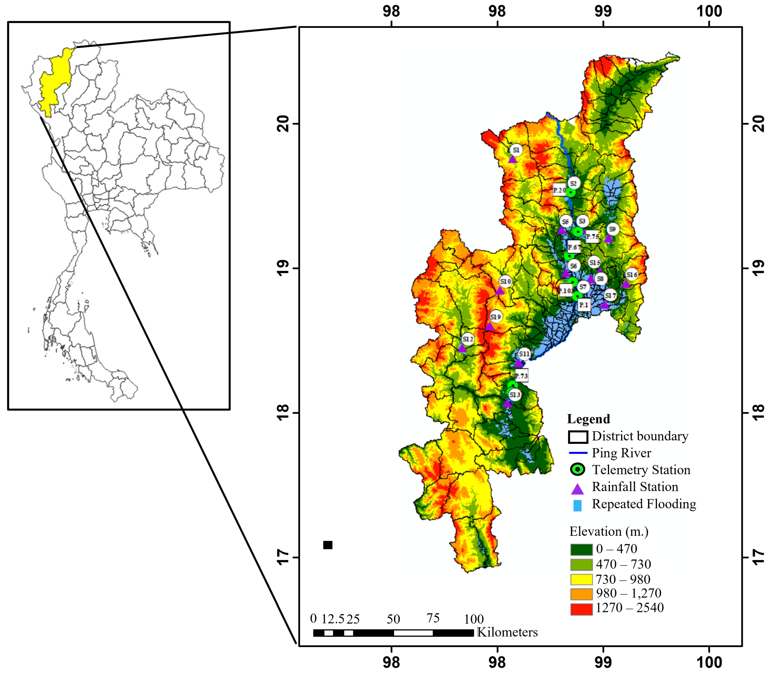
The study area is Chiang Mai Province in northern Thailand. The Ping River is the primary waterway that flows through the province and connects various economic and residential zones. The province is made up of 23 districts and 204 sub-districts, and it covers a total area of 20,107 km2. The province has a tropical monsoon climate, which means it has a distinct wet and dry season. Most precipitation occurs during the wet season, from June to September, accounting for approximately 80% of the annual rainfall. Due to the high volume of rainfall, the province is at an increased risk of flooding. The province boasts diverse landscapes, such as plains, hills, and mountains, as shown in Figure 1. The color in the figure represents an elevation in meters units: dark green indicates low elevations, such as plains, and red indicates high elevations, such as mountains, according to the color scale in the legend. Furthermore, the blue area in Figure 1 represents the regions in Chiang Mai Province susceptible to flooding. The most frequent flooding events occur in plains areas surrounding the city. Additionally, the region is covered by 14 water-level telemetry stations represented in green circles named P.95, P.20, P.92, P.75, P.67, P.93, P.21, P.80, P.103, P.1, P.81, P.84, P.82, and P.64, arranged in sequence from upstream to downstream. There are also 16 rain gauge stations representing purple triangles, including S.1, S.2, S.3, S.4, S.5, S.6, S.7, S.8, S.9, S.10, S.11, S.12, S.13, S.14, S.15, and S.16, distributed throughout the area.
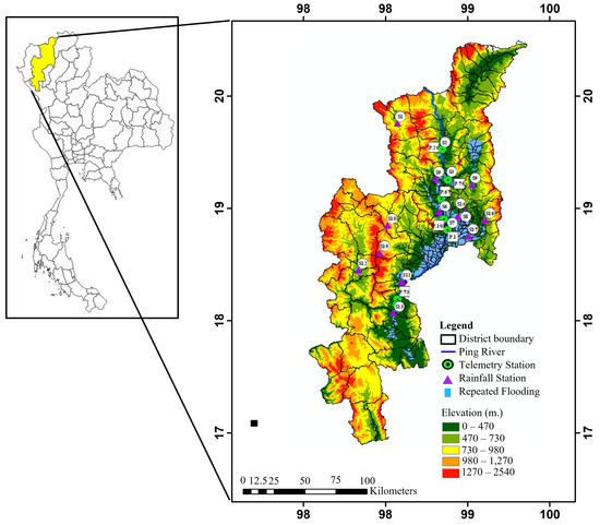
Figure 1.
Location of the study area including telemetry and rain gauge stations: Chiang Mai Province, Thailand.
2.2. Spatiotemporal Flood Hazard Map Prediction
The flood hazard map shows areas that are prone to flooding. This risk assessment is based on historical flood data and various spatial data layers in grid cells. The spatial data result from integrating the topological and statistical layers. The result of the spatial data analysis represents a period that might need to be more effective for disaster prevention due to its potential obsolescence. However, while hazard map models are effective in spatial dimensions, generating spatiotemporal predictions requires transforming temporal data into spatial data through spatial interpolation methods.
The term “spatiotemporal data” refers to information that varies in space and over time. It is related to both spatial (location-based) and temporal (time-based) aspects [5], and spatiotemporal data are essential for understanding complex systems, analyzing patterns and trends, predicting future events, and making informed decisions in various domains, including environmental information and disaster management. This comprehensive information is crucial for the analysis and visualization of spatial data. It can be applied to prediction models to estimate disaster events in each area, particularly for disasters like flash floods, climate forecasting, and forest fires. Thus, spatiotemporal prediction combines temporal prediction and can be converted into spatial interpolation with geographic information to predict flood hazard areas at risk of flooding generated with map generation techniques.
2.2.1. Map Generation Techniques
Current research on hazard maps as a tool for planning migration and emergency response can be divided into deterministic and non-deterministic methods.
Deterministic methods use mathematical equations based on fundamental principles to simulate and predict disaster behaviors. For example, in a study by [6], the Soil and Water Assessment Tool (SWAT) was used to simulate discharge and sediment transport. In [7], the TOPography-based hydrological MODEL (TOPMODEL) was used to simulate floodplain inundation. In [8], the Nested Air Quality Prediction Modeling System (NAQPMS) was used to describe regional and urban scale atmosphere pollution, employing physical and chemical simulation processes. Ref. [9] used the forest landscape simulation model (LANDIS-II) to simulate forest landscapes. However, deterministic methods are usually designed based on specific assumptions and may not accommodate various real-world conditions. Additionally, these models require detailed data that can be challenging to collect, especially for large areas.
Non-deterministic methods, including both statistical and machine learning approaches, are useful for developing predictive solutions in classification. Statistical methods like the analytical hierarchy process (AHP) [10], logistic regression (LR) [11], and frequency ratio (FR) [12], as well as machine learning methods like support vector machines (SVMs) [13], random forest (RFs) [14], and convolutional neural networks (CNNs) [15], are widely utilized for this purpose.
To summarize, there are two reasons why machine learning models perform better than statistical models, as stated in a study by [16] on wildfire prediction. Firstly, machine learning models can handle complex tasks with limited information. Secondly, they can efficiently represent large, complex, non-linear systems.
Thus, spatial data are obtained by integrating different spatial data layers, which helps interpret geographical information with machine learning. The method for generating flood maps included [17], which uses remote sensing and GIS to create floodplain maps. In recent studies, Refs. [18,19] found that CNN-based methods are more reliable and practical in producing flood susceptibility maps than conventional methods. Ref. [19] reported a 17% improvement over support vector machine (SVM) models. CNNs are faster than traditional techniques and can automatically recognize and extract intricate spatial patterns and features from spatial data. Thus, this study utilizes a CNN to generate a flood hazard map because it can learn spatial patterns, is suitable for high-dimensional data, and can process complex data.
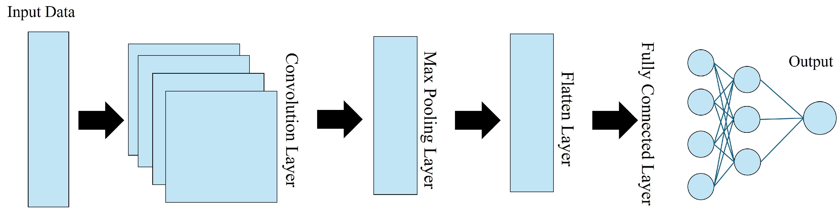
Convolution neural networks (CNNs) are powerful deep learning tools commonly used for processing images and generating maps. Their architecture has several layers, as shown in Figure 2. The input layer receives the data to be processed, while the convolution layer applies filters to extract relevant features from the input. The pooling layer downsamples the data by taking the maximum values in dimensions, and the flattened layer converts the multidimensional data into a one-dimensional vector. Finally, the fully connected layer consists of neurons connected to all neurons in the preceding layer, used for classification or regression tasks.
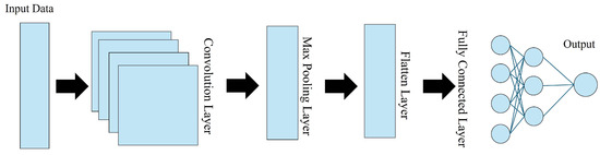
Figure 2.
The structure of the convolution neural network (CNN).
2.2.2. Temporal Prediction Techniques
The temporal prediction technique estimates future observations based on historical data applied to temporal data. There are two main categories of temporal prediction methods: statistics and machine learning. Massada [16] has shown that machine learning outperforms statistical methods on complex and non-linear data. Long short-term memory (LSTM) and artificial neural networks (ANN) are two examples of machine learning techniques. Caihong [20] compared LSTM and ANN for predicting rainfall-runoff values and concluded that LSTM produced better results than ANN. Gao [21] compared CNN, GRU, and LSTM to predict runoff without requiring time-step optimization during sample generation and found that LSTM was better than ANN and GRU.
Furthermore, many researchers have utilized LSTM to predict hydrological data by evaluating historical time series data, such as [22,23,24]. LSTM is considered a suitable method for predicting hydrological time series data due to its superior stability compared to other techniques, its ability to handle complex and non-linear data satisfactorily, and its high efficiency. This paper outlines the temporal prediction process of the LSTM technique.
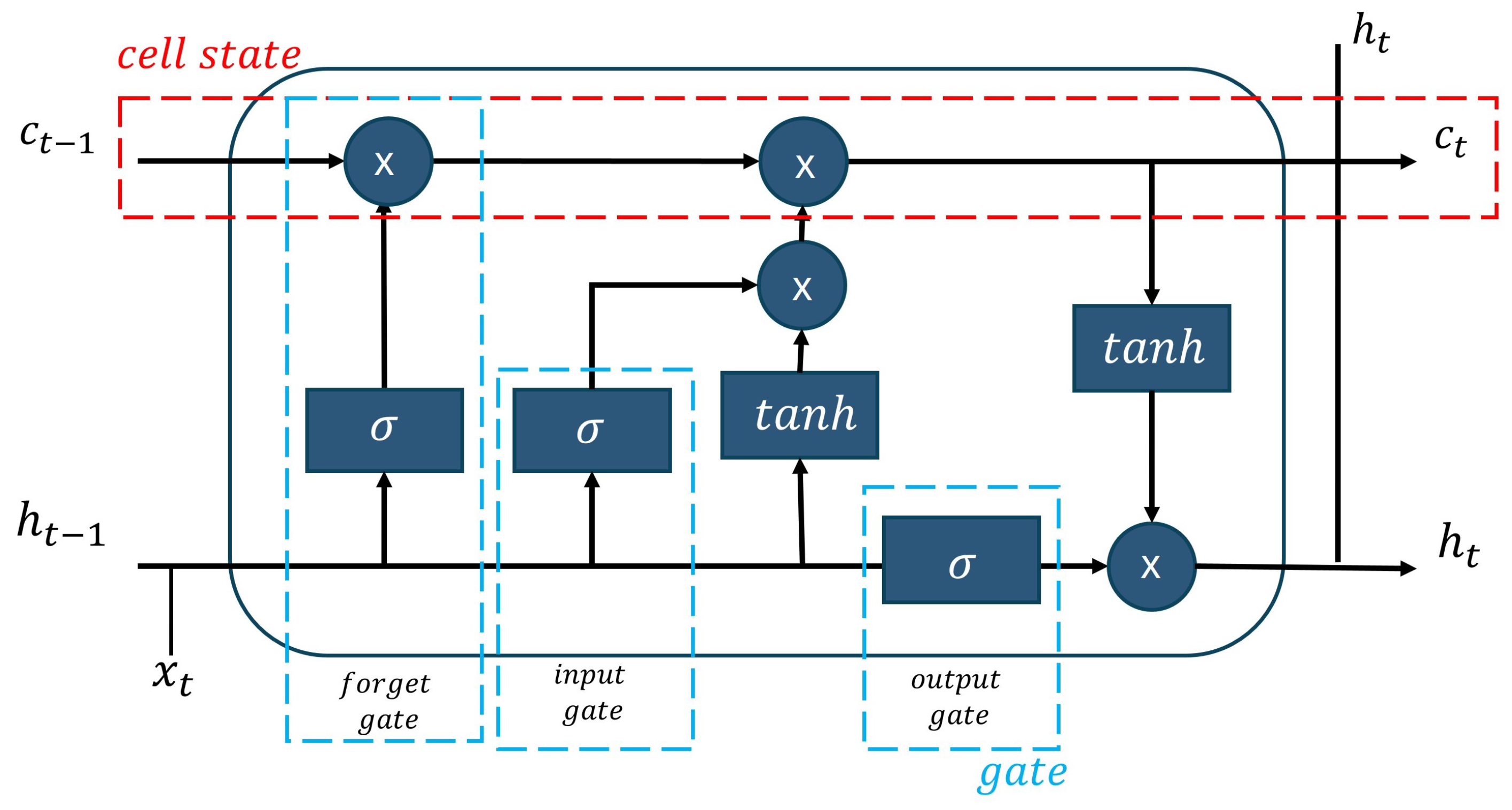
The Long Short-Term Memory (LSTM) is a recurrent neural network that can understand time series data with extended intervals and choose the most appropriate time lags for temporal prediction. The LSTM consists of cell states and gates. The memory storage unit of LSTM is known as the cell state. The gates in LSTM are responsible for controlling data flow while reading, writing, or forgetting. The gates include forgetting, input, and output gates, as depicted in Figure 3. The cell state is represented by the red dot box, and the gates are represented by three blue boxes: forget, input, and output.
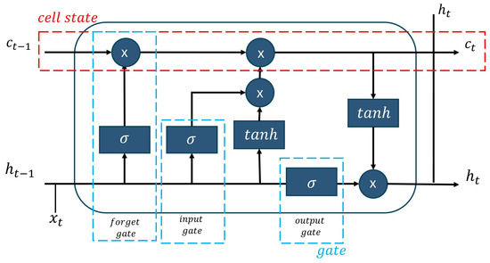
Figure 3.
The structure of long short-term memory (LSTM) technique.
Forget Gate: The forget gate decides what cell states should be forgotten. The cell state from the previous hidden state and the current input are passed through the sigmoid function. The output is a value in the range [0, 1] where 0 means forgotten and 1 means reserved. Equation (1), represents the sigmoid function; and are the weight matrix; is biased; is the input at the current time; and is the previous value of the hidden state.
Input Gate: The input gate updates the cell state. The gate applies the sigmoid and tanh functions. The output of the input gate combines the output from the forget gate and the input gate to update the cell state at time t as Equation (2). When is the output from the forget gate; ⊗ represents element-wise multiplication; the sigmoid function decides the cell state in the hidden state to update; values of W are the weight matrix; is the input at the current time t; is the previous value of the hidden state; and are biased; and the tanh activation function determines the new candidate values.
Output Gate: The output gate decides which hidden state is next taken as the output. The output of the cell can be calculated as Equation (3). When the gate uses the sigmoid function to decide which hidden state is taken as the output, and are the weight matrix, and is biased in the output state. The hidden state at time t can be updated as Equation (4) using the tanh function.
2.2.3. Spatial Interpolation Techniques
Spatial interpolation techniques are typically classified as deterministic (e.g., linear interpolation, IDW, and Spline) or non-deterministic (e.g., Kriging and Gaussian Processes). The IDW method considers that every input data point takes a localized impact that diminishes with distance weights. It assigns greater importance to closer data points, indicating they possess a higher weight. Many researchers have applied IDW to interpolate various parameters such as PM2.5 concentrations [25], soil Cadmium [26], and rainfall [27]. Moreover, the researchers used IDW to interpolate the values such as [28,29,30]. The Spline method utilizes a mathematical function to estimate values while minimizing surface curvature. This results in a smooth surface that passes exactly through the input points. In a study conducted by [31], the authors utilized spline interpolation to estimate groundwater contamination. The Kriging technique is a geostatistical interpolation method that estimates values in unknown areas by utilizing the distance and variation degree between known data points. In [32], the authors proposed that spatiotemporal changes in PM2.5 concentrations can be evaluated using different Kriging techniques, including ordinary, simple, and universal Kriging. The study found that universal Kriging is the most effective method for analyzing air pollution distributions in various areas. As a result, this technique can be extended to other regions to monitor air pollution changes over time. Ref. [33] compared interpolation methods for depth to groundwater. The results show that IDW has the lowest relative error coefficient compared to other techniques. Researchers widely favor it due to its superior accuracy compared to other methods. However, it may not be suitable for flat areas where IDW and Spline are more appropriate. Thus, this study uses IDW to extrapolate information about spatial data because it is simple , fast, and practical . It is suitable for generating flood hazard maps, enabling timely response to flood situations.
The inverse distance weighted (IDW) technique is a deterministic method used to estimate the value of unknown points based on the known points in a spatial data set [34]. To calculate the estimated values, a weighted average of the known values is taken, with the weight of each value determined by the distance between the known and unknown points, as shown in Equation (5).
where is value of the unknown point; the value of the ith known point is represented by ; N represents the total number of known points. is the weight value for each known point (i) can be determined by calculating the distance between the known and the unknown point (p).
Temporal data, such as water level and rainfall, provided as input will be used to create spatial data through the IDW interpolation for undeployed station locations in this paper.
2.3. Proposed Framework
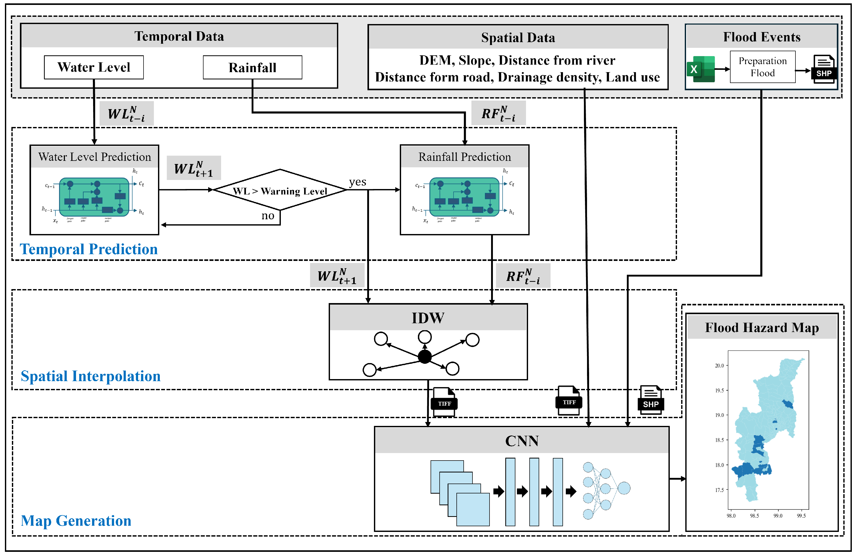
This paper proposes a framework for generating flood hazard maps. The proposed framework utilizes spatiotemporal data through interpolation from environmental monitoring stations such as telemetry stations and rain gauge stations, as well as spatial data. The framework consists of three main processes: temporal prediction, spatial interpolation, and map generation, as shown in Figure 4. The input data include both temporal and spatial information. Temporal information regarding flooding includes measurements such as water level and rainfall recorded by telemetry and rain gauge stations. Furthermore, the flood event transforms the Excel file into a spatial file, displaying the flooded area per subdistrict. This temporal prediction process uses two models using the LSTM technique to predict the likelihood of flooding: water level and rainfall. The area could flood if the expected water level exceeds the warning threshold. Therefore, the rainfall prediction model predicts rainfall values in advance when there is a possibility of flood in this area. These temporal data are converted into spatial data through the interpolation technique using the IDW technique to estimate unknown values with water level and rainfall in this area without a station. The CNN trains and acquires flood occurrence information from spatial data. Finally, the visualization process produces a hazard map displaying the predicted flood risk at the sub-district level. With its user-friendly interface, this visualization enhances the accessibility and comprehension of the predicted flood hazard information, empowering stakeholders to make informed decisions on flood risk management and mitigation strategies.
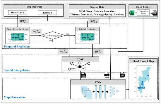
Figure 4.
The framework for spatiotemporal flood hazard map.
2.3.1. Temporal Prediction Process
This process focuses on predicting future data that affect floods from environmental monitoring stations, which are temporal data. This paper applies the LSTM technique to this process. It aims to predict values based on historical data, as shown in Figure 4, in a partial temporal data and temporal prediction technique. The input consists of water level and rainfall data, essential parameters in flood monitoring [35]. The developed process is designed to accurately predict future water and rainfall levels by leveraging past data. The process includes two prediction models. The first model predicts water levels for all telemetry stations within the study area, generating multi-output results that reflect the water levels at each station for the subsequent time step, representing where N represents the number of telemetry stations in this area and i is the previous time. These outputs consist of water level values for the next day represented as . Similarly, the second model predicts rainfall levels across all rain gauge stations in the study area represented as , providing comprehensive insights into future rainfall data representing . The output of this technique is the predicted water level and rainfall for all stations in the study area. The predictive model for flood risk will only activate if the water level exceeds the warning level, indicating a possible flooding threat in the area. Each telemetry station has its unique warning level value, and the model will continually monitor the situation. The model predicts rainfall if any station exceeds the threshold and generates the next step accordingly. Therefore, the output of this technique provides water level and rainfall data for all stations in the study area.
2.3.2. Spatial Interpolation Process
The process is shown in Figure 4, the input consists of and , which are outputs from the temporal prediction process. These temporal data are converted into spatial data through the interpolation technique. Spatial interpolation is widely used for predicting values at unknown locations based on known data points. The IDW technique estimates unknown values, such as future water levels and rainfall, based on the distance between known value stations. When there are no telemetry or rain gauge stations, the IDW technique calculates values based on the distance from the closest known station. Transforming temporal prediction output data into spatial data using the IDW technique is beneficial, as it provides valuable insights into the spatial distribution of predicted values.
2.3.3. Map Generation Process
This process follows Figure 4 in the part of map generation. This study uses geospatial data to create flood hazard maps, incorporating topographical features and real-time environmental observations. The study employs CNN to produce maps that outline subdistrict boundaries and identify areas impacted by floods within a specified study area. Using CNN to generate flood maps significantly enhances flood detection, response precision, and efficiency in diverse geographic provinces. The map generation process gathers data from spatial interpolation techniques, focusing on one day of water level and rainfall prediction. Additionally, the model considers various topographical features, such as a digital elevation model (DEM), slope, distance from the river, distance from the road, drainage density, and land use, resulting in eight features. Then, a composite band is utilized for streamlined data management by combining the eight individual bands into a single layer for simultaneous visualization and analysis of various spectral bands. The carefully curated input data are the basis for training to produce a detailed flood hazard map. Each data point within this spatial framework is a raster image, allowing the CNN to identify patterns and features. Historical flood event data are integrated into the training data set to enhance the model’s predictive capabilities. The model aims to achieve high accuracy and precision through extended training and testing. This technique leads to the development of a reliable flood map that can effectively guide proactive flood management measures.
3. Evaluation and Result
This section describes the experiment setup, evaluation, and results of the framework. Section 3.1 explains the data set and the parameter settings. Section 3.2 performance metrics and framework results, including temporal prediction and map generation.
3.1. Experiment Setup
3.1.1. Data
The Department of Disaster Prevention and Mitigation, Chiang Mai (DDPM CM), recorded flood events in this study area. The DDPM CM is responsible for collecting information on flood areas, including the date of the flood, the affected area, and the type of damage that occurred, in Excel format. These data cover the period from 2020 to 2022. To convert the data into geospatial data, village-level data are combined into sub-district data to show flooding events in each sub-district. Moreover, the DDPM CM provides data recorded from the telemetry stations and rain gauge stations; thus, there are two types of input data: temporal and spatial data.
Flood Temporal Data: the temporal data, water level, and rainfall recordings are obtained from the Upper Northern Region Irrigation Hydrology Center. These data include values from 14 telemetry stations and 16 rain gauge stations. The data cover the period from 1 April 2020 to 30 September 2022.
Flood Spatial Data: the flood spatial data consist of historical flood events and topographical spatial features. The historical flood event recorded by DDPM CM covers 2020–2022, and topographical spatial features, as shown in Figure 5, illustrate flood spatial data. The colors represent low and high values of features, including:
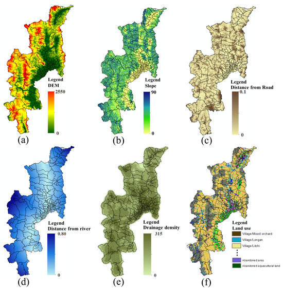
Figure 5.
Flood spatial data; (a) DEM, (b) slope, (c) distance from road, (d) distance from river, (e) drainage density, and (f) land use.
- (a)
- Digital Elevation Model (DEM): Elevation data representing terrain height. Sourced from the United States Geological Survey (https://earthexplorer.usgs.gov (accessed on 19 March 2024)).
- (b)
- Slope: Measurements of land steepness relative to horizontal. The data were obtained from the United States Geological Survey (https://earthexplorer.usgs.gov (accessed on 19 March 2024)).
- (c)
- Distance from the river and the location’s proximity to the nearest road. These data were sourced from the Open Street Map.
- (d)
- Distance from road: Proximity of location to the nearest river. These data were sourced from the Open Street Map.
- (e)
- Drainage density: Measurement of the stream network length per unit area. These data are available in the Fundamental Geographic Data Set (FGDS).
- (f)
- Land use: Categorization of surface activities on land. These data were obtained from the Land Development Department.
3.1.2. Parameter Settings
The parameter settings for the LSTM and the IDW technique are detailed in Table 1. The inputs consisted of 42 and 48 entries for the water level and rainfall prediction models, respectively, covering the data period from 1 April 2020 to 30 September 2022. The output predicts the next value at a one-time step. The data for the prediction span 678 days (80%), while the data for testing encompass 170 days (20%). The model is trained using the Adam optimizer with a learning rate of 0.00005. Additionally, the IDW technique sets input numbers 14 and 16 for water level and rainfall. The output cell size is 0.005, and the search radius point is 12 for interpolation values.

Table 1.
Temporal and spatial parameter settings.
This study used the CNN technique to analyze flooding in a particular study area. The input and parameter settings of the CNN technique are presented in Table 2, which provides detailed information about the model’s configuration. The data set used for this study consists of 4080 images, each representing a subdistrict and having a dimension of 33 × 33 × 8. We allocated 10 days for training, 6 days for validation, and 4 days for testing, with 204 images per day. The model comprises five layers in depth, with two pooling sizes and dense layers of sizes 120 and 86, respectively. The activation function used in the model is ReLU.
Table 2.
CNN parameter settings.
The framework was developed with Python version 3.12 using added libraries including sklearn, matplotlib, pandas, geopandas, keras, rasterio, pyidw, and geometry. The hardware uses a virtual machine service from the university; it has an Intel(R) Xeon(R) Gold 6254 vCPU @ 3.10 GHz with 64 cores (Intel Corporation, Santa Clara, CA, USA), 64 GB of RAM, and an Nvidia Tesla V100 8 GB vGPU (Nvidia Corporation, Santa Clara, CA, USA).
3.2. Evaluation
3.2.1. Performance Metrics
Root mean squared error (RMSE) measures the standard deviation of residuals. It is the square root of the average squared difference between the actual and predicted values as explained in Equation (6).
where is the actual value, is the predicted value, and n is number of observations.
Mean absolute error (MAE) measures the average of the residuals. It is the average absolute difference between the actual and predicted values as explained in Equation (7).
where is the actual value, is the predicted value, and n is the number of observations.
The R-squared value (R2 or the coefficient of determination) measures the proportion of variance of the target that the model. The value of R2 ranges from 0 to 1, where 0 means that none of the variability in the target variable is explained by the features used in the model, and a value of 1 means that the model perfectly explains all of the variability in the target variable using the features. The R2 can be calculated by Equation (8).
where is the actual value, is the predicted value, is the average of the actual value, and n is the number of observations.
A confusion matrix summarizes the performance of a classification model consisting of the number of true positives (TP), true negatives (TN), false positives (FP), and false negatives (FN) in the prediction model. The confusion matrix technique can calculate metrics including accuracy, precision, recall, and F1-score, which can be described as follows:
(1) Accuracy is a measure of the overall performance of a model and represents the ratio of correctly predicted observations to the total number of observations.
(2) Precision is the ratio of correctly predicted positive observations to the total.
(3) Recall is the proportion of true positives to all actual positives.
(4) F1-score is a single metric for measuring the performance of modeling.
3.2.2. Temporal Prediction Evaluation
The temporal prediction technique has been evaluated using three metrics: RMSE, MAE, and R2. The evaluation results are presented in Table 3. The evaluation is performed at iterations between 100 and 1000 of two models, including water and rainfall predictions. The average metric values are presented for the models’ training and testing in Table 3. The water level prediction model result achieved an RMSE of 0.028 and 0.135 for training and testing, respectively. The MAE values were 0.013 and 0.071 for training and testing, respectively. Additionally, the R2 values were 0.843 and 0.624. On the other hand, the rainfall prediction model achieved an RMSE of 0.044 and 0.196, an MSE of 0.021 and 0.112, and R2 values of 0.766 and 0.610 for training and testing, respectively. The models achieved R2 scores exceeding 0.6, indicating a good fit for the data [36]. Thus, both models exhibit high accuracy in predicting future values, as evidenced by the low error levels. Consequently, these models may be considered dependable and reliable tools for optimizing decision-making processes. In addition, the box plot graph presented in Figure 6 provides an insightful view of the LSTM models’ training process for predicting water level and rainfall. The graph shows a decrease in RMSE scores as the number of iterations during training increases, indicating an improvement in the accuracy of the predictions.
Table 3.
Temporal prediction performance evaluation in 2020–2022.
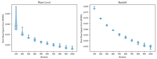
Figure 6.
RMSE of water level and rainfall prediction training process.
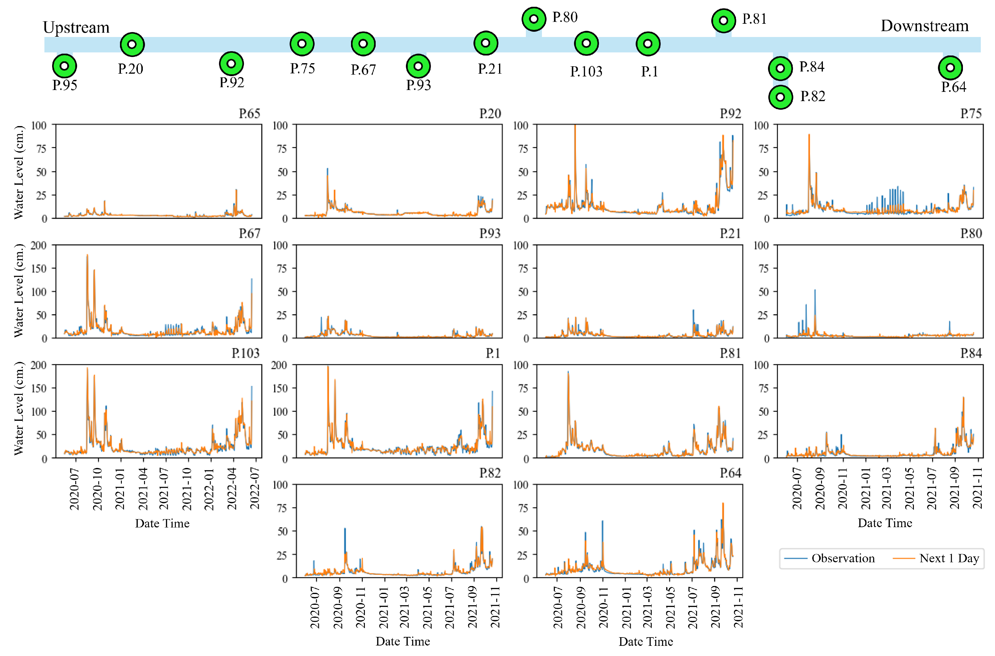
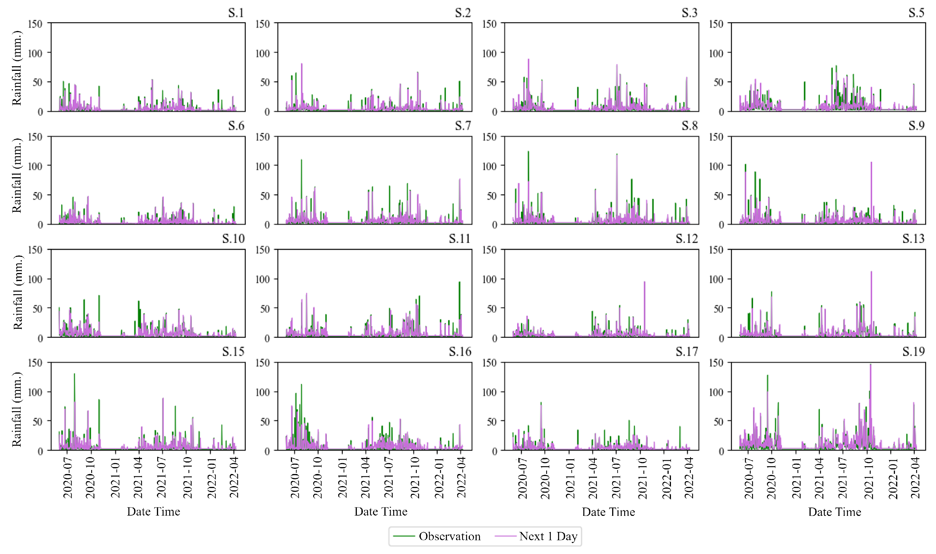
In Figure 7 (top), the image above shows the river network and the telemetry station locations. On the left is the upstream section of the river, while the right side shows the downstream section. Six primary stations are installed on the main river, namely P.20, P.75, P.67, P.21, P.103, and P.1. Additionally, other stations are located on the branch river. The bottom multi-graph in Figure 7 (bottom) represents water level predictions resulting from the training process. Each graph represents water levels at 14 telemetry stations in Chiang Mai Province. The green line represents the observed values, while the orange line depicts the predicted values. These graphs depict peaks in water levels during the years 2020–2021. Three to four hydrograph peaks may cause flooding during observation periods due to higher levels than usual. Similarly, Figure 8 displays a sample of rainfall predictions from the training process model. Each graph represents rainfall at 16 stations. The green line denotes observed values, while the purple line represents predicted values. These graphs show peaks in rainfall levels during the years 2020–2021. When observed, there will be much rain during the month of July to October , which is the rainy season in Thailand.
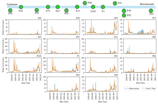
Figure 7.
The river network and telemetry station location (top) and graph comparison between actual and predicted water level data using LSTM at the training process of the telemetry stations during 2020–2021 in Chiang Mai Province (bottom).
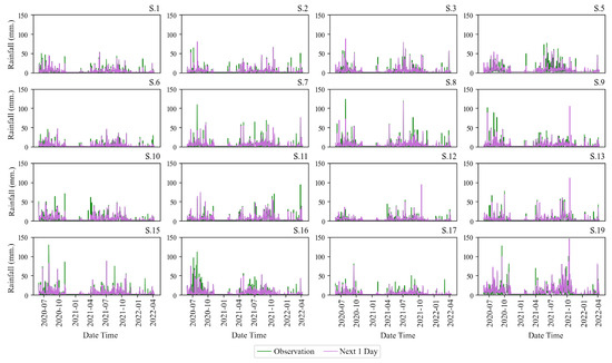
Figure 8.
The actual and predicted rainfall data using LSTM at the training process of the rainfall gauge stations during 2020–2021 in Chiang Mai Province.
3.2.3. Map Generation Evaluation
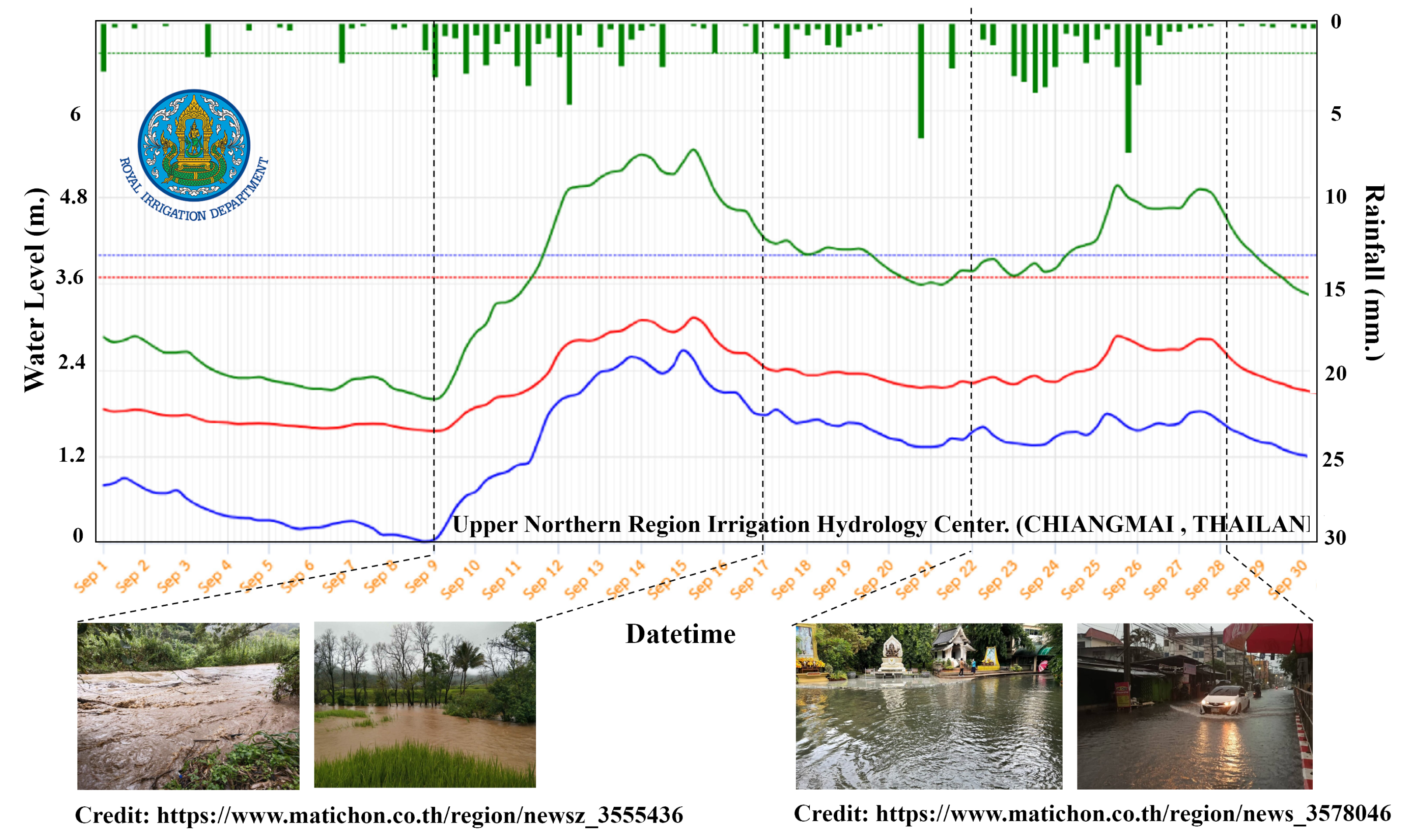
The performance of a model was evaluated using a confusion matrix, which included accuracy, precision, recall, and F1-score. The evaluation used four-day testing data coinciding with flooding events and heavy rainfall, including 10–11 and 23–24 September 2022. The times referenced from the Upper Northern Region Hydrology Center (Chiang Mai, Thailand) and Matichon news (https://www.matichon.co.th/ (accessed on 19 March 2024)) are depicted in Figure 9. The graph shows water levels measured at telemetry stations installed on the Ping river, where the blue line is P.67, the red line is P.1, and the green line represents P.103 represents. The rainfall is represented by a green-colored histogram. The figure indicates significant fluctuations and rainfall quantities. These peak hydrographs are flooding incidents in the mentioned area. The results of this evaluation are presented in Table 4, indicating that all metrics scored above 0.9. The model’s accuracy, precision, recall, and F1-score are 0.953, 0.976, 0.941, and 0.974, respectively. The high scores suggest that the model can accurately predict and map flood hazards in the area.
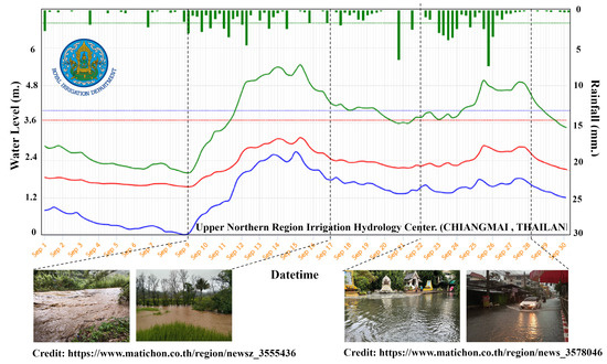
Figure 9.
The water level and rainfall information from the Upper Northern Region Hydrology Center and the Matichon news (accessed on 19 March 2024).
Table 4.
Confusion metric of map evaluation on 10–11, 23–24 September 2022.
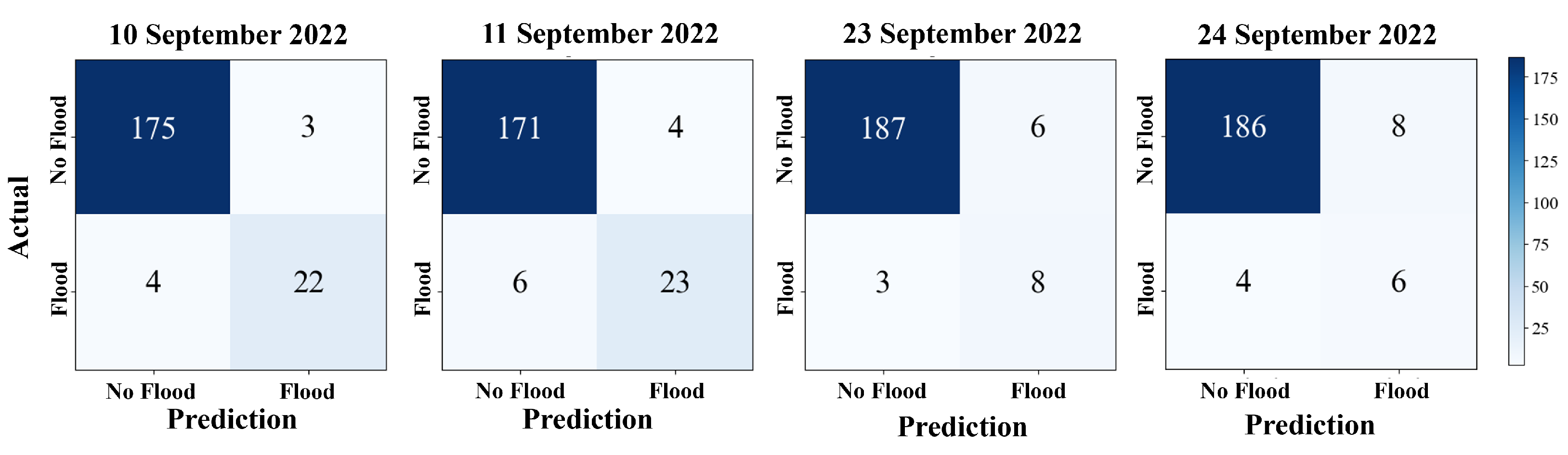
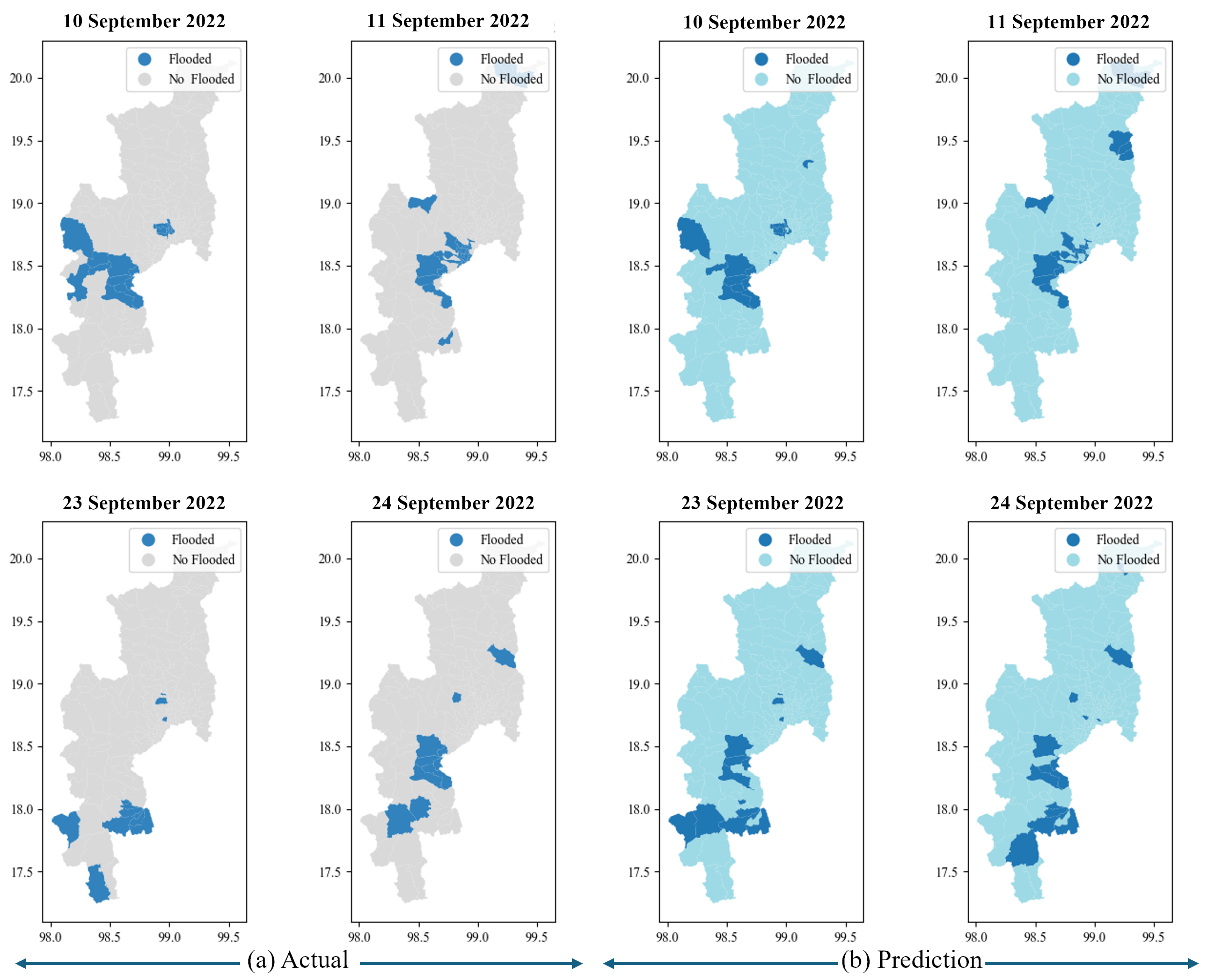
Moreover, Figure 10 details each confusion matrix value. It indicates the accuracy of the flood predictions compared to the actual situation. The total 204 represent sub-districts. For example, on 10 September 2022, a flood occurred in 26 sub-districts, with predicted floods in 22 sub-districts. There are false negatives in three sub-districts and false positives in four sub-districts. Additionally, there were no floods in 175 sub-districts. On 11 September 2022, 29 sub-districts were flooded. The model can be predicted to be 23 flooded. There are false negatives in four sub-districts and false positives in six sub-districts. In contrast, on September 23 and 24, flooding occurred in 11 and 10 sub-districts, respectively. The model predicts true negatives, false positives, and false negatives in similar sub-districts. Nonetheless, the model have give highly accurate predictions close to the actual situation. Figure 11, the flood hazard map illustrates the flooding occurrences in Chiang Mai province between 10 and 11 and 23–24 September 2022. The comparison between (a) actual flooding data indicated in navy blue and no floods indicated in gray is obtained from the Chiang Mai Provincial Disaster Prevention Department. Flooding predicted by the model is depicted in (b). The navy blue area represents flooding, and during these dates, the area in Chiang Mai faced actual flooding situations.

Figure 10.
Detail of confusion metric of map evaluation on 10–11, 23–24 September 2022.
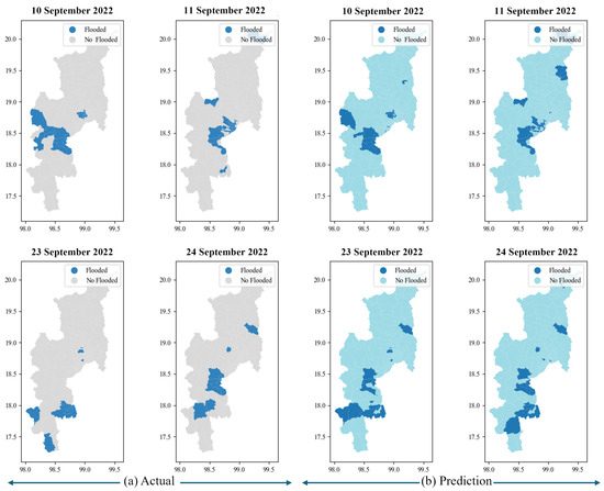
Figure 11.
Comparison between the actual flood event (a) and predicted flood event (b) represented with a flood hazard map on 10–11 and 23–24 September 2022.
4. Discussion
4.1. Temporal Prediction Process
The temporal prediction technique uses LSTM models to predict water levels and rainfall. The results of the water level prediction, as shown in Table 4, indicates a model error at 0.028–0.135 which is equivalent to water level amounts of around 10–40 cm for both training and testing, measured by RMSE and MAE at 0.013–0.071 which is equivalent to water level amounts of approximately 5–25 cm for water level prediction. Rainfall prediction has RMSE between 0.044 and 0.196 which is equivalent to rainfall amounts of approximately 8–38 mm. MAE at 0.021–0.112 which is equivalent to rainfall amounts of approximately 4–21 mm. Moreover, when considering the value, the models exhibit variance ranging from 0.62 to 0.84, signifying a relatively good performance. However, when considering the test data in detail, it is found that the low values may be due to test data that have not been trained before. Periods under intense scrutiny face adverse weather conditions, with rainfall and water levels significantly higher than normal during the upcoming rainy season of 2022.
Considering that the data used for training may be insufficient for this model, more historical data should be considered, perhaps using data from the past 10 years or when the study area experienced significant flooding within the study area. However, extending the data set becomes challenging due to the limited data collected from only a few monitoring stations within the study area. Only five years’ worth of data covering both water level and rainfall are available from the 14 telemetry stations and 16 rain gauge stations, posing a constraint on data availability within this study area.
Additionally, the multi-output models for prediction may influence the model inaccuracies, while one model can predict across all monitoring stations, it might lead to higher errors compared to using one model per station. However, employing individual models for each station may generate higher accuracy but must be traded off with a longer computational time.
In conclusion, to improve the accuracy of the prediction models, it is recommended to enhance the historical data set by incorporating more extensive temporal data, consider the trade-offs between using multi-output models and compare individual models for each monitoring station, keeping in mind the computational resources required for processing.
4.2. Map Generation Process
This map generation process creates a flood hazard map using a CNN. This model has highly effective results, as indicated by the high F1-score of 0.974. This represents the accuracy in predicting areas prone to flooding in the future. The model indicates the ability to differentiate between flood and no-flood areas efficiently. However, errors such as false positives and false negatives may occur due to minimal variations in geographic and water level or rainfall that do not significantly impact the predictions.
Furthermore, it is predicted that IDW’s spatial interpolation may result in an imperfect flood prediction if the available telemetry and rain gauge stations are inadequate. A dearth of data hampered the accuracy of this prediction model, leading to highly unreliable forecasts. To overcome this limitation, obtaining more information on flood-prone areas from the relevant agencies is imperative, as the current data used in the study are inadequate. With more comprehensive data, the model’s efficacy can be enhanced.
To improve the model’s accuracy, it is essential to integrate larger data sets into the training process and incorporate additional relevant data on flood-prone areas, such as recurring flood occurrences, temperature data, and spatially related information. However, caution is crucial when utilizing unreliable data, which can significantly affect the model’s accuracy. Regular updates to the model are also vital to ensure it can effectively respond to flood events.
4.3. Framework
The proposed framework has been designed to assist the agencies responsible for monitoring disasters in the Chiang Mai area, such as the Provincial Disaster Prevention Department, the Municipality, the Sub-district Administrative Organization, and the Upper Northern Region Irrigation Hydrology Center. Flood Hazard maps that utilize spatiotemporal data can provide high accuracy and responsiveness to flooding hazards, which helps organizations prepare effectively for flood situations. Although we may not be able to prevent such incidents from occurring, we can mitigate their impact by providing warning notifications to residents, directing evacuations to higher ground, and constructing high water walls to prevent overflow and flooding. Therefore, if we have highly accurate predictions and responsiveness to flood risk areas, we can work towards reducing future losses. Moreover, this framework can be applied in other areas, but measuring stations must cover the entire area and collect data on flooded areas. With this information available, a model can be created with high accuracy and responsiveness to flood events before they occur.
5. Conclusions
This research paper presents a framework for creating a spatiotemporal flood hazard map prediction using machine learning for flood early warning. The framework involves two main processes: temporal prediction and spatial data interpolation. Long Short-Term Memory (LSTM) is used for the temporal prediction process to forecast future water levels and rainfall. In the spatial data interpolation process, the Inverse Distance Weighting (IDW) technique estimates the missing values. The final flood hazard map is prepared by integrating spatiotemporal data, which includes temporal data (i.e., water level and rainfall) and spatial data (i.e., DEM, slope, distance from the river, distance from the road, drainage density, and land use). The study area is Chiang Mai Province, Thailand, covering 20,107 square kilometers. The study uses data from 14 water-level stations and 16 rain gauge stations operated by the Upper Northern Region Irrigation Hydrology Center in Chiang Mai, Thailand. These stations provide temporal data. The framework’s effectiveness is evaluated using performance metrics (i.e., RMSE, MAE, and R2) for the temporal prediction technique. For map generation evaluation, a confusion matrix is used to evaluate water level, rainfall, and six geography features as input. The models consistently achieved high accuracy scores, with R2 values exceeding 0.6, indicating a goodness of fit of the data. The map generation evaluation includes water level, rainfall, and six geography features as input. The results all show values above 0.90, meaning the model has high scores, signifying its capability to predict and map flood hazards in the area accurately.
The study highlights the significance of utilizing advanced predictive modeling techniques in flood management and disaster preparedness efforts. The suggested approach is useful for understanding and mitigating flood damage by providing accurate and timely information to agencies and communities. This enables them to take proactive measures to minimize the impact of flooding events.
In the future, the study aims to investigate the possibility of generating flood maps by combining satellite imagery with additional flood data from relevant agencies. This integration is necessary because the availability of historical flood data is limited, which results in imbalanced datasets. Additionally, the maps will indicate the intensity levels of flood occurrences.
Author Contributions
Conceptualization, P.P. and P.C.; methodology, P.P. and P.C.; validation, P.P. and P.C.; formal analysis, P.P.; investigation, P.P.; resources, P.P.and P.C.; data curation, P.P.; writing—original draft preparation, P.P.; writing—review and editing, P.C.; visualization, P.P. and P.C.; supervision, P.C.; project administration, P.C. All authors have read and agreed to the published version of the manuscript.
Funding
This research received no external funding.
Institutional Review Board Statement
Not applicable.
Informed Consent Statement
Not applicable.
Data Availability Statement
The data presented in this study are available on request from the corresponding author.
Acknowledgments
This work was supported by the CMU HPC Erawan Project, Information Technology Service Center (ITSC), Chiang Mai University, Chiang Mai, Thailand. The authors would like to thank ITCS for its computing resources. The Upper Northern Region Irrigation Hydrology Center (Chiang Mai, Thailand) for archiving the data and providing access to environmental data.
Conflicts of Interest
The authors declare no conflict of interest.
References
- The Meteorological Department Flood. Available online: https://www.tmd.go.th/info/info.php?FileID=70 (accessed on 17 October 2022).
- CRED. Natural Disasters 2020. Available online: https://reliefweb.int/report/world/cred-crunch-newsletter-issue-no-70-april-2023-disasters-year-review-2022 (accessed on 17 October 2022).
- Reyes, M.V.; Sarsycki, M. Disaster Risk Assessment Guideline. Available online: https://disaster.go.th/upload/download/file_attach/58a6b30dd6232.pdf (accessed on 19 March 2024).
- Ganguly, M.; Aynyas, R.; Nandan, A.; Mondal, P. Hazardous area map: An approach of sustainable urban planning and industrial development—A review. Nat. Hazards 2018, 91, 1385–1405. [Google Scholar] [CrossRef]
- Zhong, S.; Wang, C.; Yu, Z.; Yang, Y.; Huang, Q. Spatiotemporal exploration and hazard mapping of tropical cyclones along the coastline of China. Adv. Meteorol. 2018, 2018, 5479576. [Google Scholar] [CrossRef]
- Oeurng, C.; Sauvage, S.; Sánchez-Pérez, J.M. Assessment of hydrology, sediment and particulate organic carbon yield in a large agricultural catchment using the SWAT model. J. Hydrol. 2011, 401, 145–153. [Google Scholar] [CrossRef]
- Li, W.; Lin, K.; Zhao, T.; Lan, T.; Chen, X.; Du, H.; Chen, H. Risk assessment and sensitivity analysis of flash floods in ungauged basins using coupled hydrologic and hydrodynamic models. J. Hydrol. 2019, 572, 108–120. [Google Scholar] [CrossRef]
- Wang, Z.; Maeda, T.; Hayashi, M.; Hsiao, L.F.; Liu, K.Y. A nested air quality prediction modeling system for urban and regional scales: Application for high-ozone episode in Taiwan. Water Air Soil Pollut. 2001, 130, 391–396. [Google Scholar] [CrossRef]
- Sturtevant, B.R.; Scheller, R.M.; Miranda, B.R.; Shinneman, D.; Syphard, A. Simulating dynamic and mixed-severity fire regimes: A process-based fire extension for LANDIS-II. Ecol. Model. 2009, 220, 3380–3393. [Google Scholar] [CrossRef]
- Harshasimha, A.C.; Bhatt, C.M. Flood vulnerability mapping using maxent machine learning and analytical hierarchy process (AHP) of Kamrup Metropolitan District, Assam. Environ. Sci. Proc. 2023, 25, 73. [Google Scholar] [CrossRef]
- Lee, J.Y.; Kim, J.S. Detecting areas vulnerable to flooding using hydrological-topographic factors and logistic regression. Appl. Sci. 2021, 11, 5652. [Google Scholar] [CrossRef]
- Cao, C.; Xu, P.; Wang, Y.; Chen, J.; Zheng, L.; Niu, C. Flash flood hazard susceptibility mapping using frequency ratio and statistical index methods in coalmine subsidence areas. Sustainability 2016, 8, 948. [Google Scholar] [CrossRef]
- Singha, C.; Swain, K.C.; Meliho, M.; Abdo, H.G.; Almohamad, H.; Al-Mutiry, M. Spatial analysis of flood hazard zoning map using novel hybrid machine learning technique in Assam, India. Remote Sens. 2022, 14, 6229. [Google Scholar] [CrossRef]
- Antzoulatos, G.; Kouloglou, I.O.; Bakratsas, M.; Moumtzidou, A.; Gialampoukidis, I.; Karakostas, A.; Lombardo, F.; Fiorin, R.; Norbiato, D.; Ferri, M.; et al. Flood hazard and risk mapping by applying an explainable machine learning framework using satellite imagery and GIS data. Sustainability 2022, 14, 3251. [Google Scholar] [CrossRef]
- Liu, J.; Liu, K.; Wang, M. A residual neural network integrated with a hydrological model for global flood susceptibility mapping based on remote sensing datasets. Remote Sens. 2023, 15, 2447. [Google Scholar] [CrossRef]
- Massada, A.B.; Syphard, A.D.; Stewart, S.I.; Radeloff, V.C. Wildfire ignition-distribution modelling: A comparative study in the Huron–Manistee National Forest, Michigan, USA. Int. J. Wildland Fire 2012, 22, 174–183. [Google Scholar] [CrossRef]
- Amini, J. A method for generating floodplain maps using IKONOS images and DEMs. Int. J. Remote Sens. 2010, 31, 2441–2456. [Google Scholar] [CrossRef]
- Wang, Y.; Fang, Z.; Hong, H.; Peng, L. Flood susceptibility mapping using convolutional neural network frameworks. J. Hydrol. 2020, 582, 124482. [Google Scholar] [CrossRef]
- Youssef, A.M.; Pradhan, B.; Dikshit, A.; Mahdi, A.M. Comparative study of convolutional neural network (CNN) and support vector machine (SVM) for flood susceptibility mapping: A case study at Ras Gharib, Red Sea, Egypt. Geocarto Int. 2022, 37, 11088–11115. [Google Scholar] [CrossRef]
- Hu, C.; Wu, Q.; Li, H.; Jian, S.; Li, N.; Lou, Z. Deep learning with a long short-term memory networks approach for rainfall-runoff simulation. Water 2018, 10, 1543. [Google Scholar] [CrossRef]
- Gao, S.; Huang, Y.; Zhang, S.; Han, J.; Wang, G.; Zhang, M.; Lin, Q. Short-term runoff prediction with GRU and LSTM networks without requiring time step optimization during sample generation. J. Hydrol. 2020, 589, 125188. [Google Scholar] [CrossRef]
- Wilbrand, K.; Taormina, R.; ten Veldhuis, M.C.; Visser, M.; Hrachowitz, M.; Nuttall, J.; Dahm, R. Predicting streamflow with LSTM networks using global datasets. Front. Water 2023, 5, 1166124. [Google Scholar] [CrossRef]
- Gauch, M.; Kratzert, F.; Klotz, D.; Nearing, G.; Lin, J.; Hochreiter, S. Rainfall–runoff prediction at multiple timescales with a single Long Short-Term Memory network. Hydrol. Earth Syst. Sci. 2021, 25, 2045–2062. [Google Scholar] [CrossRef]
- Shrestha, S.G.; Pradhanang, S.M. Performance of LSTM over SWAT in Rainfall-Runoff Modeling in a Small, Forested Watershed: A Case Study of Cork Brook, RI. Water 2023, 15, 4194. [Google Scholar] [CrossRef]
- Ma, J.; Ding, Y.; Gan, V.J.; Lin, C.; Wan, Z. Spatiotemporal prediction of PM2.5 concentrations at different time granularities using IDW-BLSTM. IEEE Access 2019, 7, 107897–107907. [Google Scholar] [CrossRef]
- Sheng, J.; Yu, P.; Zhang, H.; Wang, Z. Spatial variability of soil Cd content based on IDW and RBF in Fujiang River, Mianyang, China. J. Soils Sediments 2021, 21, 419–429. [Google Scholar] [CrossRef]
- Giarno; Didiharyono, D.; Fisu, A.A.; Mattingaragau, A. Influence rainy and dry season to daily rainfall interpolation in complex terrain of Sulawesi. IOP Conf. Ser. Earth Environ. Sci. 2020, 469, 012003. [Google Scholar] [CrossRef]
- Prathom, C.; Champrasert, P. General circulation model downscaling using interpolation—Machine learning model combination—Case study: Thailand. Sustainability 2023, 15, 9668. [Google Scholar] [CrossRef]
- Yang, F.; Huang, G.; Li, Y. A New Combination Model for Air Pollutant Concentration Prediction: A Case Study of Xi’an, China. Sustainability 2023, 15, 9713. [Google Scholar] [CrossRef]
- Akbar, T.A.; Javed, A.; Ullah, S.; Ullah, W.; Pervez, A.; Akbar, R.A.; Javed, M.F.; Mohamed, A.; Mohamed, A.M. Principal Component Analysis (PCA)–Geographic Information System (GIS) modeling for groundwater and associated health risks in Abbottabad, Pakistan. Sustainability 2022, 14, 14572. [Google Scholar] [CrossRef]
- Shyamala, G.; Arun Kumar, B.; Manvitha, S.; Vinay Raj, T. Assessment of spatial interpolation techniques on groundwater contamination. In Proceedings of the International Conference on Emerging Trends in Engineering (ICETE) Emerging Trends in Smart Modelling Systems and Design, Hyderabad, India, 22–23 March 2019; Springer: Berlin/Heidelberg, Germany, 2019; pp. 262–269. [Google Scholar] [CrossRef]
- Rusmili, S.H.A.; Mohamad Hamzah, F.; Choy, L.K.; Azizah, R.; Sulistyorini, L.; Yudhastuti, R.; Chandraning Diyanah, K.; Adriyani, R.; Latif, M.T. Ground-Level Particulate Matter (PM2.5) Concentration Mapping in the Central and South Zones of Peninsular Malaysia Using a Geostatistical Approach. Sustainability 2023, 15, 16169. [Google Scholar] [CrossRef]
- Sun, Y.; Kang, S.; Li, F.; Zhang, L. Comparison of interpolation methods for depth to groundwater and its temporal and spatial variations in the Minqin oasis of northwest China. Environ. Model. Softw. 2009, 24, 1163–1170. [Google Scholar] [CrossRef]
- Maleika, W. Inverse distance weighting method optimization in the process of digital terrain model creation based on data collected from a multibeam echosounder. Appl. Geomat. 2020, 12, 397–407. [Google Scholar] [CrossRef]
- Orozco, M.M.; Caballero, J.M. Smart disaster prediction application using flood risk analytics towards sustainable climate action. MATEC Web Conf. 2018, 189, 10006. [Google Scholar] [CrossRef]
- Moksony, F.; Heged, R. Small is beautiful. The use and interpretation of R2 in social research. Szociol. Szemle Spec. Issue 1990, 130–138. [Google Scholar]


Disclaimer/Publisher’s Note: The statements, opinions and data contained in all publications are solely those of the individual author(s) and contributor(s) and not of MDPI and/or the editor(s). MDPI and/or the editor(s) disclaim responsibility for any injury to people or property resulting from any ideas, methods, instructions or products referred to in the content. |
© 2024 by the authors. Licensee MDPI, Basel, Switzerland. This article is an open access article distributed under the terms and conditions of the Creative Commons Attribution (CC BY) license (https://creativecommons.org/licenses/by/4.0/).