Optimization Study of Soil Organic Matter Mapping Model in Complex Terrain Areas: A Case Study of Mingguang City, China

Abstract

Traditional soil organic matter mapping is mostly polygonal drawing, which is even more difficult to accurately depict in complex terrain areas. The spatial distribution of soil organic matter is closely related to agricultural production, natural resources, environmental governance, and socio-economic development. Efficiently, economically, and accurately obtaining information on changes in soil organic matter in areas with diverse topography is an urgent problem to be solved. Mingguang City has a high research value because of its unique topography and natural landscape. To solve the problem of soil organic matter mapping in this area, this study will construct an excellent organic matter prediction model. Using 173 soil survey samples (123 for training and 50 for testing), the optimal feature variable subsets selected from 31 environmental variables through Pearson correlation, stepwise regression-variance inflation factor, and recursive feature elimination models based on different algorithms were employed. Each selected feature subset was then used to construct organic matter prediction models using multiple advanced machine learning algorithms. By comparing accuracy validation and model performance, the organic matter prediction model suitable for Mingguang City (RFE-RF_SVM) was obtained, that is, the prediction model of organic matter based on support vector machines with the feature variables screened by the feature recursive elimination algorithm of random forest with RMSE = 3.504, VSI = 0.036, and R-squared = 0.730. Furthermore, the analysis focused on assessing the significance of the predictive factors. The mapping results of this study show that the soil organic matter content in the central and northwestern parts of the study area is low, and the reasons for this situation are different. The central part is mainly caused by the change of land use and topography, while the northwestern part is caused by the loose soil structure caused by the parent material. The government can take targeted measures to improve the soil in the areas with poor organic matter.

1. Introduction

Soil is the material basis of human production and life, and organic matter is an important part of the soil solid phase. It can bind mineral soil particles tightly together and improve the physical structure of soil [1]. Soil organic matter (SOM) in a broad sense refers to the decomposition and synthesis of organic compounds by various animal, plant and microbial residues in the soil. It is the main source of nutrients for plants. Within a certain range of content, organic matter content is a good way to reflect the level of high and low soil fertility [2,3]. Therefore, the content of SOM is extremely important for agricultural production and land productivity evaluation [4,5]. In the last century, to investigate the organic matter content level of a certain piece of land, it was necessary to collect a significant amount of samples for laboratory determination, which was labor-intensive, arduous, and could not be popularized on a large scale [6]. The geostatistical method can simulate the spatial autocorrelation model and use the collected soil sample information for spatial interpolation to obtain the distribution map of regional SOM content, which provides a basis for regional soil fertility assessment [7,8]. The SoilGrids system only uses 150,000 sample data to obtain the global spatial distribution map of soil organic matter with the support of the organic matter prediction model constructed by XGBoost, Nnet and RF algorithms, and its efficiency and accuracy are incomparable to those of previous geostatistical models [9]. Nowadays, digital soil mapping technology based on the machine learning model can predict a large range of soil information through the simulation of discrete and sparse typical sample points, providing the possibility of timely and accurate acquisition of regional soil information [10]. For example, using 1014 surface soil sample data, we use the Boruta method to filter the characteristics of a huge set of environmental variables and predict the spatial distribution of soil organic matter in Florida based on eight machine learning models [11].

Digital soil mapping has received increasing attention, and with the deepening of research, global soil scholars have continuously developed mapping techniques. From random forest algorithms to innovative approaches combining with adaptive spline functions, or from new modeling ideas to extending the mapping level from two-dimensional soil surface to three-dimensional soil body attribute mapping [9,12,13], these are accompanied by the application of new algorithms, making digital soil attribute mapping enter an unprecedented period of explosive growth. There are many studies on mapping in complex terrain such as mountains, plains, or both, but there are still few and unevenly distributed soil survey points, while the situation where plains, hillsides, and low mountains are abundantly distributed within the mapping area remains a blank spot. Under such circumstances, how to accurately predict the spatial distribution of SOM is still a challenging problem. The organic matter mapping in the region that divides China into northern and southern regions is a typical example. The terrain is diverse and complex, with numerous factors affecting the soil-forming environment. The objective of this study is to develop a model that can draw a spatial distribution map of SOM in complex terrain with scarce and unevenly distributed soil survey points, providing a solution for organic matter mapping and exploring the environmental control factors that affect its spatial distribution variation.

2. Materials and Methods

2.1. Study Area

The study area is located between 32°26′51″ N–33°13′15″ N and 117°49′27″ E–118°25′32″ E, which falls within the range of the north-south demarcation line in China. The total area is 2335 km², with a cultivated land area of 1106 km², accounting for 47% of the region. The area is influenced by the Tanlu fault zone and is rich in mineral resources. The topography and landforms are unique and complex, with a general trend of high in the south and low in the north. The low mountainous area in the south is part of the watershed between the north and south of China, accounting for 35% of the region. It belongs to a semi-humid monsoon climate transitioning from northern subtropical to warm temperate, with four distinct seasons, rain and heat occurring simultaneously in the identical season. The mean yearly temperature is 15 °C, and the accumulated temperature above 0 °C is 5470 °C. The average annual rainfall is 934.1 mm, mainly concentrated in summer. The area has experienced multiple tectonic movements, and its geological structure is situated at the intersection of the North China Platform and the Yangtze Platform. The exposed strata in the area can be divided into two major rock series: Precambrian basement metamorphic rocks and Mesozoic-Cenozoic continental clastic rocks and volcanic rocks. The crop planting structure is diverse, with wheat being the main crop in the north and rice being the main food crop in the central and southern regions. In addition, there are also mung beans, corn, and mugwort planted. There are about 200 species of woody plants and more than 1000 species of herbaceous plants. The vegetation in the southern region is dominated by coniferous forests, deciduous broadleaf forests, and mixed forests of deciduous and evergreen broadleaves. The formed forest ecosystem provides abundant habitats for animals and plants. There are significant spatial differences in natural landscapes and land use patterns within Mingguang County, presenting three geographical patterns with clear boundaries but staggered distributions (Figure 1) [14]. Through the above elaboration, the study area generally presents a geographical spatial arrangement pattern of plain terrain in the north, hillock terrain in the middle and hills and mountains in the south. Among them, the average elevation of the plain area is only a few meters, the hillock is tens of meters high, and the hills are hundreds of meters. The whole study area covers a variety of different landforms, which has high research value.

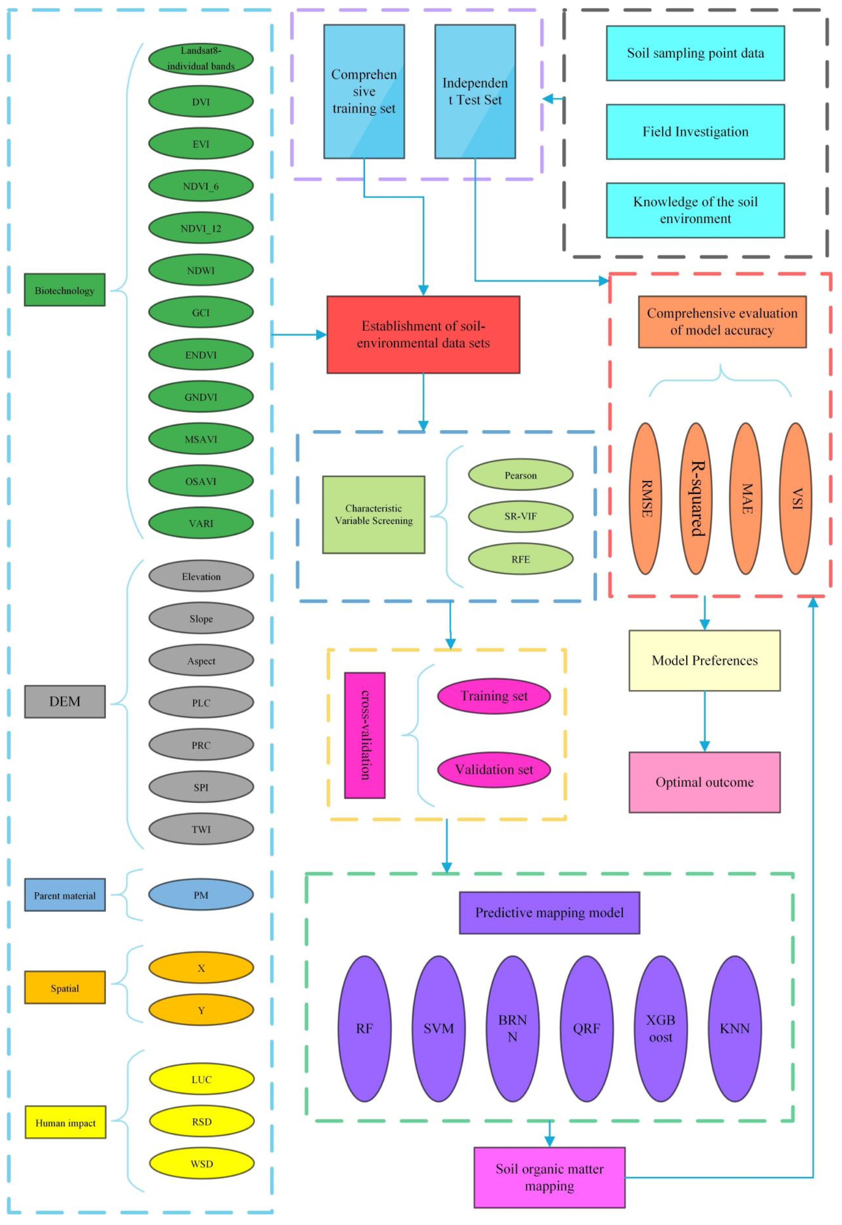
2.2. Database and Methodology

The following data were used to create the basic database in this study: Landsat 8 OLI remote sensing images (30 m resolution) for June and December downloaded from the United States Geological Survey (USGS, Reston, VA, USA) and a 30 m × 30 m digital elevation model (DEM); second soil survey data (soil type map) for the study area came from Mingguang Soil and Fertilizer Workstation; a total of 173 soil sampling sites were set up throughout the region. In order to ensure the stability and typicality of the soil sample sites, most sample points are distributed in a concentrated and contiguous cultivated layer of cultivated land. After air-drying and sieving in the laboratory, the potassium dichromate (K₂Cr₂O₇) oxidation-capacity method was used for determination (

Table 1. Data used for research and analysis.

Data Types	Environmental Factor	Definition	Spatial Resolution	Source
Biotechnology	Band_1	Landsat8-individual bands	30 m	USGS
	Band_2
	Band_3
	Band_4
	Band_5
	Band_6
	Band_7
	DVI	Difference Vegetation Index		Remote sensing image-derived data
	EVI	Enhanced Vegetation Index
	NDVI_6	Normalized Difference Vegetation Index-June
	NDVI_12	Normalized Difference Vegetation Index-December
	NDWI	Normalized Difference Water Index
	GCI	Green Chlorophyll Vegetation Index
	ENDVI	Extended normalized difference vegetation index
	GNDVI	Normalized Green Difference Vegetation Index
	MSAVI	Modified Soil Adjustment Vegetation Index
	OSAVI	Optimization Of Soil Regulatory Vegetation Index
	VARI	Visible-band Difference Vegetation Index
Topographical	Elevation	Digital elevation model model		Geospatial Data Cloud
	Slope	Degree of surface inclination		DEM-derived data
	Aspect	The direction in which the slope faces
	PLC	Plan Curvature
	PRC	Profile Curvature
	SPI	Stream Power Index
	TWI	Topographic Wetness Index
Parent material	PM	Soil map deep-dive		Local soil map
Spatial	X	Longitudes		Data from the Third Territorial Survey
	Y	Dimension
Human impact	LUC	Land Use Structure
	RSD	Residential Site Distance
	WSD	Water Source Distance

).

There are significant differences in terrain, landforms, and crop planting structures within the study area. In order to obtain realistic spatial distribution characteristics of organic matter with minimal sampling costs, the prediction results of SOM prediction models based on K-nearest neighbors, support vector machines, random forests, quantile random forests, XGboost, and neural network algorithms were compared to find an optimal solution. Before model construction, the training set and test set were randomly split in R using the caret package at a ratio of 70% and 30%, respectively. The training set was utilized for the machine learning model training, whereas the test set was used to independently assess the precision of the prediction results. Secondly, evaluation metrics such as R2, root mean square error (RMSE), and mean absolute error (MAE) were used to assess the performance of the prediction models and select the best mapping model (Figure 2).

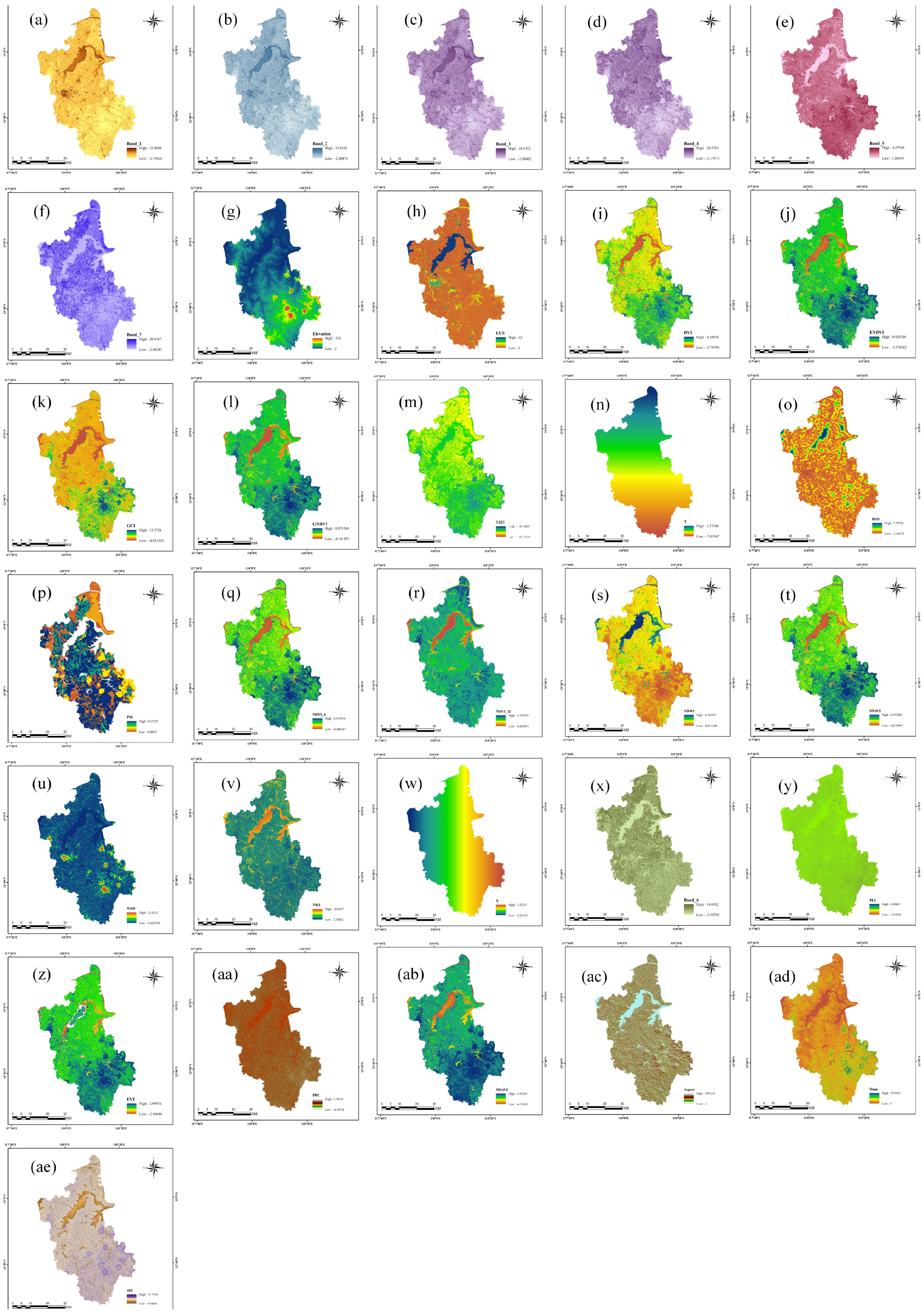
2.3. Extraction of Organic Matter Influencing Factors

According to the soil-forming factor theory of Dokuchaev, the formation and development of soil are influenced by soil-forming factors, so the soil properties at any stage are the historical comprehensive results of the influence of these factors [15]. Thus, the following aspects were considered to extract a data set related to SOM content [7].

2.3.1. Biological Factors

Biological factors are the main influencing factors in the soil-forming process. In the soil-forming process, living organisms must appear in the parent material and influence soil formation by participating in the accumulation of SOM and the formation of soil structure, which is closely related to the formation of organic matter. Under certain conditions, the growth of vegetation can be understood as a specific characterization of SOM content. After plants wither and enter the soil, they form a positive feedback with SOM content, which can be characterized by remote sensing bands, vegetation indices, distribution of vegetation types, etc. [16,17].

The research area belongs to summer in June, and the growth of plants has a good correlation with SOM. Landsat8 OLI is a land imaging instrument that can express ground data well and extract remote sensing image band data in June 2021. The band data includes image data of bands 1 to 7 (B1–B7). Band 1 Coastal (Band_1, 0.433–0.453 μm, Figure 3a) is mainly used for coastal zone observation, but it can reflect vegetation information; Band 2 Blue (Band_2, 0.450–0.515 μm, Figure 3b) is mainly used for water penetration, which can eliminate the influence of summer rainwater accumulation and identify soil vegetation; Band 3 Green (Band_3, 0.525–0.600 μm, Figure 3c) can distinguish vegetation well; Band 4 Red (Band_4, 0.630–0.680 μm, Figure 3d), Band 5 NIR (Band_5, 0.845–0.885 μm, Figure 3e), Band 6 SWIR 1 (Band_6, 1.560–1.660 μm, Figure 3x) have good explanatory power for the growth, biomass and type of ground vegetation, respectively; Band 7 SWIR 2 (Band_7, 2.100–2.300 μm, Figure 3f) not only reflects vegetation coverage and moist soil, but also can distinguish rock minerals.

In addition, remote sensing-derived vegetation index data are a simple and empirical measure of surface vegetation conditions, mainly relying on the larger reflection difference between green vegetation in the NIR band and the R band [18]. Commonly used indices include DVI (Figure 3i), EVI (Figure 3z), NDVI (Figure 3q,r), and NDWI (Figure 3s). We attempt to introduce GCI (Figure 3k), ENDVI (Figure 3j), GNDVI (Figure 3l), MSAVI (Figure 3ab), OSAVI (Figure 3t), VARI (Figure 3m) and other indices to observe whether they have a positive impact on the prediction model.

2.3.2. Terrain Factors

Altitude has a certain limitation on the accumulation of SOM, which indirectly controls the input and output of organic matter synthesis by affecting the distribution and development environment of surface plants. The 30 m resolution DEM (Figure 3g) can effectively describe the elevation spatial distribution within the area, where the research area is between 2 and 324 m in altitude. In addition, as a form of basic elevation data, the DEM derives various specialized data sets [19].

The slope is a key factor that affects the accumulation and loss of soil nutrients. Organic matter in steep terrain tends to have lower organic matter content than that in flat areas, which is due to the migration of organic matter in the soil under the action of gravity and water flow. The increase in slope enhances the migration effect, and the opportunity for SOM loss also increases. In the study area, the slope ranges from 0° to 39.92°, with the largest slope in the low mountainous area in the south-central part. A slope map was calculated and drawn using ArcGIS10.6 software (Figure 3ad).

Aspect determines the duration of sunlight and the intensity of solar radiation received by surface vegetation, further affecting photosynthesis and humification processes. Slope aspect is the angle between the projection of the normal to a tangent plane at a point on the ground in the horizontal plane and the north direction at that point. A slope aspect map was calculated and drawn using ArcGIS10.6 software (Figure 3ac). Slope aspect between 0° and 180° is east slope, while 180°–360° is west slope [20].

PLC (plan curvature) is mainly used to express the degree of terrain relief and changes in surface shape, which affects the distribution and convergence of water flow. The convergence area has a higher probability of soil moisture, which may lead to SOM loss. A planar curvature map was calculated and drawn using ArcGIS10.6 software (Figure 3y). Positive values represent transverse bumps, negative values represent transverse depressions, and zero represents linear surfaces [21].

PRC (profile curvature) is parallel to the slope and determines the rate at which water flows across the slope. If the rate is too fast, it can lead to soil erosion, while a slower rate is beneficial for sediment formation [22]. ArcGIS10.6 software calculates and draws a profile curvature map (Figure 3aa), with negative values representing uplift and low velocity, positive values representing downwarping and increased velocity, and zero representing linearity.

SPI is an index that measures the intensity of water flow, describing the distribution, rate, and potential for soil erosion by water flow [23]. ArcGIS10.6 software calculates and draws a Stream Power Index map (Figure 3ae), with the formula:

$$SPI=SCA\times Tan\left(slope\right)$$

(1)

SCA represents sink flow per unit area and slope represents slope (in degrees) [24].

TWI is a physical indicator of the impact of regional terrain on the direction and accumulation of runoff. A higher TWI indicates stronger runoff capacity at that location, which increases the risk of soil erosion and organic matter loss [25]. ArcGIS10.6 software calculates and draws a Topographic Wetness Index map (Figure 3v), with the formula:

$$TWI=In\left[SCA/Tan\left(slope\right)\right]$$

(2)

SCA, slope as above [24].

2.3.3. Parent Material Factors

As the material source of soil, the composition of PM (soil parent material) will directly affect the development and properties of soil. Due to the difficulty in directly obtaining the spatial distribution map of parent material, it is generally replaced by geological maps indirectly. At all scales of mapping, parent material is used as the basic and distinguishing characteristics of soil types, which is a very important environmental variable for soil [26]. Through understanding the process of soil development and deeply mining the internal information of soil map, the spatial distribution characteristics of PM can be extracted (Figure 3p).

2.3.4. Anthropogenic Factors

Anthropogenic factors, also known as anthropogenic environmental covariates, refer to the general term for human production activities that have a profound impact on soil development. For example, long-term cultivation of rice by humans leads to alternating oxidation-reduction reactions, material leaching and deposition in the soil, resulting in the transformation into paddy soil and changes in the direction and process of soil development. Good field management can improve the physical and chemical properties of soil, affecting texture, bulk density, soil porosity, and nutrient content. In the past decade, China has promoted the construction of high-standard farmland nationwide, mainly through transforming small fields into large ones, large-scale land leveling, improving irrigation and drainage facilities, and investing heavily in organic fertilizers, all of which have had a certain impact on soil development. In this paper, LUS (land use structure) data [27] (Figure 3h), RSD (residential site distance) data [28] (Figure 3o), and WSD (water source distance) (Figure 3u) are used as anthropogenic environmental covariates [29].

2.3.5. Spatial Factors

Soil properties vary with different spatial locations, which is essentially due to the difference in hydrothermal conditions at different spatial locations. However, there are many factors that affect hydrothermal conditions, making it extremely difficult to obtain accurate information on their changes. According to the first law of geography, everything is interrelated, but the degree of correlation decreases with increasing distance, and vice versa [7]. Therefore, spatial location not only can replace hydrothermal conditions, but also can express the spatial correlation of organic matter. Spatial location raster data with a resolution of 30 m were created based on the latitude and longitude of the study area (Figure 3w,n).

2.4. Model Building

The working principle of digital SOM mapping is highly unified with the processing idea of machine learning. For huge and complex soil attribute information, machine learning algorithms can well express their internal relationships, speculate soil information in unknown areas, and another advantage is to efficiently process complex nonlinear relationships between soil information and environmental information [30].

2.4.1. Modeling Method

k-Nearest Neighbor (KNN) Algorithm

The k-nearest neighbor (KNN) algorithm calculates the similarity between input sample points using Euclidean Distance, Manhattan Distance, or Minkowski Distance. In all feature spaces of the sample, the majority vote of k closest neighbors confirms the ownership of the variable [31]. This algorithm can be used for both classification and regression problems. Its advantages are simple algorithm, inclusive of outliers, capable of handling nonlinear problems, and effective in dealing with different types of cross-sample. The selection of k value in classification and regression needs to be carefully considered. Generally, the lower the k value (k ≥ 1), the greater the model complexity, the more sensitive it is to sample noise, and the weaker its generalization ability. Conversely, it can use cross-validation to determine the appropriate k value. This study uses R4.3.2 software to build a KNN algorithm model and analyzes the accuracy of the model in expressing SOM distribution.

Support Vector Machine

The support vector machine (SVM) is a generalized linear classifier for the binary classification of data, which is based on the Vapnik–Chervonenkis (VC) dimension theory and structural risk minimization principle. For nonlinear problems, SVM can use kernel functions to construct high-dimensional mappings of input data and determine the optimal parameters of the kernel function through cross-validation [32]. Commonly used kernel functions include polynomial kernel (PK), radial basis function kernel (PBFK), and linear kernel (LK). In this study, a support vector machine model was constructed using a radial basis kernel, with the regularization parameter C playing a decisive role. The expression of the radial basis function is:

$$K(x,y)=\exp (-\gamma \Vert x-y{\Vert }^2)$$

(3)

where γ is a positive parameter and ||x − y|| is the Euclidean distance between two vectors. By adjusting the value of γ, you control the width and shape of the radial basis function, which in turn affects the performance of the SVM [33].

Random Forest

Random forests are composed of multiple classification and regression trees, each of which is independent and unaffected by the others. During training, individual sample sets are selected from the training data set, and feature variables are used as explanatory variables for the model. All trees randomly select a splitting rule for confirming tree nodes and vote on the result based on a certain deterministic averaging process. Random forests can be used to handle both classification and regression problems, and they also support continuous and discrete data. Their advantage lies in their strong generalization ability, making them suitable for model fitting and simulation of data with low bias and high variance. They have good prediction accuracy on a global scale or within small watersheds [34]. In R4.3.2 software, the caret package is used to build random forest models, outputting feature importance rankings to analyze the contribution level of feature variables.

Quantile Random Forest

Quantile regression forests is an ensemble learning method based on decision trees proposed by Nicolai for regression analysis [35]. Unlike the random forest algorithm, it not only considers the predicted values of each sample in the training set, but also takes into account the distribution of the predicted values to better understand the uncertainty and diversity of the data. That is, while each test sample enters the decision tree prediction, the quantiles of all decision tree predictions are calculated, and, when integrating, the predicted values of all numbers are weighted and averaged according to the quantiles, with the final output result. The quantile is any real number, generally taking values such as 0.1, 0.25, 0.5, 0.75, 0.9, etc. The weights can be adjusted according to the size of the quantile. The advantage of this model is that it considers the distribution of predicted values, captures data uncertainty more effectively, effectively reduces variance and bias, and has high stability [36]. In this paper, the quantile regression forests model was created using the caret package in R4.3.2 software to analyze the model results.

XGBoost

XGBoost is an efficient and flexible advanced supervised algorithm based on the boosting framework. It is an optimized distributed gradient boosting decision tree algorithm proposed by Tianqi Chen et al., which is similar to gradient boosting decision trees, but optimizes parallel computing efficiency, missing value handling, and prediction performance. It can handle various types of structured and semi-structured heterogeneous data. Typically, greedy or approximate algorithms are used for splitting, and the splitting of nodes depends on the change in information gain. If the change is positive, the node is split; if it is negative, it is not. In addition, additional regularization terms and support for row and column sampling are added when calculating the loss function to smooth the model and avoid overfitting. The advantages of this model are that it can obtain global optimal solutions, perform cross-validation during iterations, and effectively handle missing values [37]. In this study, we used R4.3.2 software to build XGBoost models and train them to obtain optimal parameters.

Neural Network

The neural network is a computer model that abstracts the interconnection between human brain neurons. It consists of several layers of neurons, each of which processes information from the earlier layer through weighted summation and activation function processing before passing it on to the next layer of neurons. The overall structure can be summarized as input layer, hidden layer, and output layer, mainly used to solve complex problems. Its training process includes multiple iteration cycles, each of which performs forward propagation and backward propagation once, and adjusts weights and biases based on the current loss function value [38,39]. This study used Bayesian regularized neural networks (BRNNs) for model prediction, in which uncertainty was introduced into the weights for regularization, and an infinite number of neural networks on the ensemble weight distribution were used for prediction [40]. In R4.3.2 software, a Bayesian neural network analysis was performed on organic matter sample information, and the algorithm was optimized.

2.4.2. Variable Selection

In this study, in order to explore which variable screening method can help improve the precision of the model, three methods were selected: Pearson correlation coefficient (PCC), stepwise regression-variance inflation factor (SR-VIF) and recursive feature elimination (RFE).

The association between all variables was investigated using the Pearson correlation coefficient [41,42], which was used to measure the correlation between SOM content and all environmental variables. The relationship was quantitatively expressed with a numerical range of −1 to 1, where 1 represents complete positive correlation, −1 represents complete negative correlation, and 0 indicates no correlation. The calculation formula is:

$$\mathrm{pearson}=\mathrm{sqrt}\left[\right(n\times \sum xy)/(n\times \sum x^2)-(\sum x{)}^2\left)\right]$$

(4)

Among them, Pearson represents the correlation coefficient between Pearson, n represents the number of samples, ∑xy represents the covariance between two variables, ∑x² represents the variance of a variable, and ∑x represents the mean value of a variable. Pearson correlation analysis was performed in R4.3.2 software to explore which environmental variables are closely related to SOM content from the data and assist in subsequent variable screening [43].

The SR-VIF method can automatically select the most important variables from the variable set. Its core idea is to introduce each independent variable one by one, and after introducing a new independent variable, it is necessary to test the original independent variables and remove those whose regression sum of squares are not significant. In this paper, the stepwise regression selection method was used as backward method, with Akaike information criterion (AIC) as the screening standard [44,45]. This standard can balance the complexity of the model and the effect of model fitting data, that is, the lower the AIC value, the better the model’s fit. On this basis, variance inflation factor (VIF) was connected to further detect multicollinearity of variables. Finally, the variables retained in the model were both important and not seriously collinear [46].

RFE is a search algorithm that repeatedly builds models, traverses all features to discover the optimal combination, and obtains the global optimal solution for actual effects. Its most important aspect is the repeated recursive training of models, eliminating weak features, i.e., removing feature variables that have no positive impact on model prediction performance and accuracy [47]. In this study, we built RFE models based on K-nearest neighbors, support vector machines, random forests, quantile random forests, XGBoost, and neural network algorithms in R4.3.2 software. We used cross-validation to evaluate feature importance and used this importance as the criterion for feature variable.

RFE is a Brute force search method that repeatedly builds models, traverses all features to find the best combination, and obtains the global optimal solution for actual effects [48]. Its most important aspect is the repeated recursive training of models, eliminating weak features, i.e., removing feature variables that have no positive impact on model prediction performance and accuracy [47]. In this study, we built RFE models based on K-nearest neighbors, support vector machines, random forests, quantile random forests, XGBoost, and neural network algorithms in R4.3.2 software. We used cross-validation to evaluate feature importance and used this importance as the criterion for feature variable reduction.

2.4.3. Accuracy Verification

For the SOM content prediction models built by K-nearest neighbors, support vector machines, random forests, quantile random forests, XGBoost and neural network algorithms, three indicators of MAE [49], RMSE [50] and R-squared [51] are used for accuracy evaluation. The sum of the differences between each actual value and predicted value is called MAE, and the smaller its value, the smaller the deviation between the predicted value and the actual value, indicating a better fit of the model; the square root of the sum of the squares of the differences between each actual value and predicted value is called RMSE; R-squared is calculated through Total Sum of Squares (TSS) and Residual Sum of Squares (RSS), with the formula as follows:

$$R‐\mathrm{squared}=1-(RSS/TSS)$$

(5)

Among them, TSS represents the total variability of the dependent variable, and RSS represents the variability of the residuals that cannot be explained by the regression model. The value range is between 0 and 1, with 0 representing poor fit and no connection, and 1 representing perfect fit [52].

These three accuracy evaluation criteria are somewhat related. MAE and RMSE are used as auxiliary discrimination indicators, with no specific hard standards, and the smaller the value in relative situations, the better. R² also has no specific division requirements, and different evaluation objectives have different standards. Its numerical value can well express the goodness of fit. For the prediction of SOM content, generally, if the accuracy reaches above 0.5, it indicates that the model is available and has a good fitting effect. In addition to calculating accuracy by dividing the training set and test set within the model training process, an additional test set is still reserved to calculate accuracy for comparison purposes to avoid overfitting of the model [50].

In addition, in order to find the optimal mapping model, this study constructs variance summary indices (VSIs) as a reference for model selection. The formula of VSI is as follows:

$$VSI=\left|RMSE{ }_M-RMSE{ }_T\right|+\left|R{‐\mathrm{squared} }_{\mathrm{M}}-R{‐\mathrm{squared} }_{\mathrm{T}}\right|$$

(6)

where RMSE_M is the RMSE of a certain training model, RMSE_T is the RMSE of the trained model on the test set, R-squared_M represents R-squared on the training set, and R-squared_T represents R-squared on the test set. The value of VSI is a real number greater than or equal to zero, with a smaller value indicating stronger generalization ability and higher stability of the model. When the value is zero, it means that the model can perfectly capture the underlying distribution or pattern of the data.

3. Results and Analysis

3.1. Selection of Limiting Factors of SOM

3.1.1. PCC Selection Results

There are a total of 31 covariates in the overall environmental variable set. The linear correlation between each variable and organic matter was calculated using the Pearson coefficient, and the results are shown in

Table A1. Results of correlation between environmental variables and organic matter content.

Factors	Pearson	Factors	Pearson
Band_1	−0.790	RSD	0.215
Band_2	−0.809	MSAVI	−0.024
Band_3	−0.795	PM	−0.254
Band_4	−0.753	NDVI_6	−0.026
Band_5	−0.759	NDVI_12	0.148
Band_6	−0.810	NDWI	−0.204
Band_7	−0.834	OSAVI	−0.026
Elevation	−0.321	Slope	0.051
LUS	−0.171	PLC	0.104
DVI	−0.579	PRC	−0.042
ENDVI	−0.167	Aspect	−0.249
EVI	−0.037	SPI	0.017
GCI	0.199	WSD	0.017
GNDVI	0.204	TWI	−0.066
VARI	−0.268	X	0.172
Y	0.244

. The positive or negative sign only represents positive or negative correlation, and it should be converted to absolute value for comparison. The analysis results show that seven bands in Landsat8 OLI had a significant negative correlation with SOM, with absolute values ranging from 0.753 to 0.834, which had high reference significance. In addition, DVI and Elevation had a high negative correlation with SOM, with absolute values of 0.579 and 0.321, respectively; the absolute values of correlation coefficients of most other variables were between 0.1 and 0.3, indicating weak correlation, limited explanatory power for SOM, and that they can only play a certain auxiliary role; variables such as EVI, MSAVI, NDVI_6, OSAVI, Slope, Profile Curvature, SPI, Water Source Distance and TWI had very weak correlation with SOM, with coefficient absolute values less than 0.1, and their impact is minimal.

The Pearson coefficient only calculates the correlation numerically and cannot directly delete variables with weak correlation based on this result, because some variables may show better performance in the model. In this study, we mainly selected variables with a relatively strong correlation, so we used the condition of Pearson coefficient greater than 0.1 as the variable screening condition, and we obtained the variables for model training by ourselves [53,54].

3.1.2. SR-VIF Selection Results

Step-to-step regression analysis screened out 11 variables from 31 variables to get the best feature subset. The results of the subset are shown in

Table A2. Step by step regression of AIC index value of each combination.

Stepwise Variable Combination	AIC
Band_5 + DVI + Band_1 + Band_2 + Band_3 + Band_6 + Band_7 + NDWI + Elevation + LUS + ENDVI + EVI + GCI + RSD + MSAVI + PM + NDVI_6 + NDVI_12 + OSAVI + Slope + PLC + PRC + Aspect + SPI + WSD + TWI + VARI + X + Y	314.69
Band_5 + DVI + Band_1 + Band_2 + Band_3 + Band_6 + Elevation + LUS + ENDVI + RSD + MSAVI + PM + NDVI_6 + NDVI_12 + OSAVI + Slope + PLC + PRC + Aspect + SPI + WSD + TWI + VARI + X + Y	306.77
Band_5 + DVI + Band_1 + Band_2 + Band_3 + Band_6 + Elevation + LUS + ENDVI + PM + NDVI_6 + NDVI_12 + OSAVI + PLC + PRC + Aspect + SPI + WSD + TWI + VARI + X + Y	301.18
Band_5 + Band_1 + Band_2 + Band_3 + Band_6 + Elevation + LUS + ENDVI + PM + NDVI_6 + NDVI_12 + OSAVI + Aspect + SPI + WSD + TWI + VARI + X + Y	295.96
Band_5 + Band_2 + Band_3 + Band_6 + Elevation + LUS + ENDVI + PM + NDVI_6 + NDVI_12 + OSAVI + Aspect + SPI + WSD + TWI + VARI + X + Y	294.40
Band_5 + Band_2 + Band_3 + Band_6 + Elevation + LUS + ENDVI + PM + NDVI_6 + NDVI_12 + OSAVI + SPI + WSD + VARI + Y	290.07
Band_5 + Band_2 + Band_3 + Band_6 + Elevation + LUS + ENDVI + PM + NDVI_12 + OSAVI + SPI + WSD + Y	287.47
Band_5 + Band_2 + Band_3 + Elevation + ENDVI + PM + NDVI_12 + OSAVI + SPI + WSD + Y	286.13

, and the coefficients of each variable in the model are shown in

Table A3. Stepwise regression feature variable coefficients and collinear results.

Factors	Iinear Regression Coefficient	VIF
Band_5	−12.782	26.023
Band_2	−9.110	16.079
Band_3	7.117	32.159
Elevation	−0.095	1.805
ENDVI	−151.364	7.266
PM	−7.202	1.620
NDVI_12	4.928	1.661
OSAVI	125.731	13.555
SPI	0.179	1.123
WSD	1.378	1.164
Y	−0.850	2.329

.

The variance collinearity analysis of the 11 selected variables is shown in Table A3. The results indicate that Band_5 (VIF = 26.023), Band_2 (VIF = 16.079), Band_3 (VIF = 32.159), and OSAVI (13.556) all have values greater than 10, indicating that these four variables are collinear and may impact the model’s correctness negatively. However, when comparing the collinearity analysis results with the Pearson correlation analysis results, it was found that the variables that need to be deleted are highly correlated with SOM. Therefore, instead of directly deleting the variables with high collinearity, they were divided into various scenarios and analyzed in depth by incorporating them into the model, and a final decision was made on which ones to keep or discard.

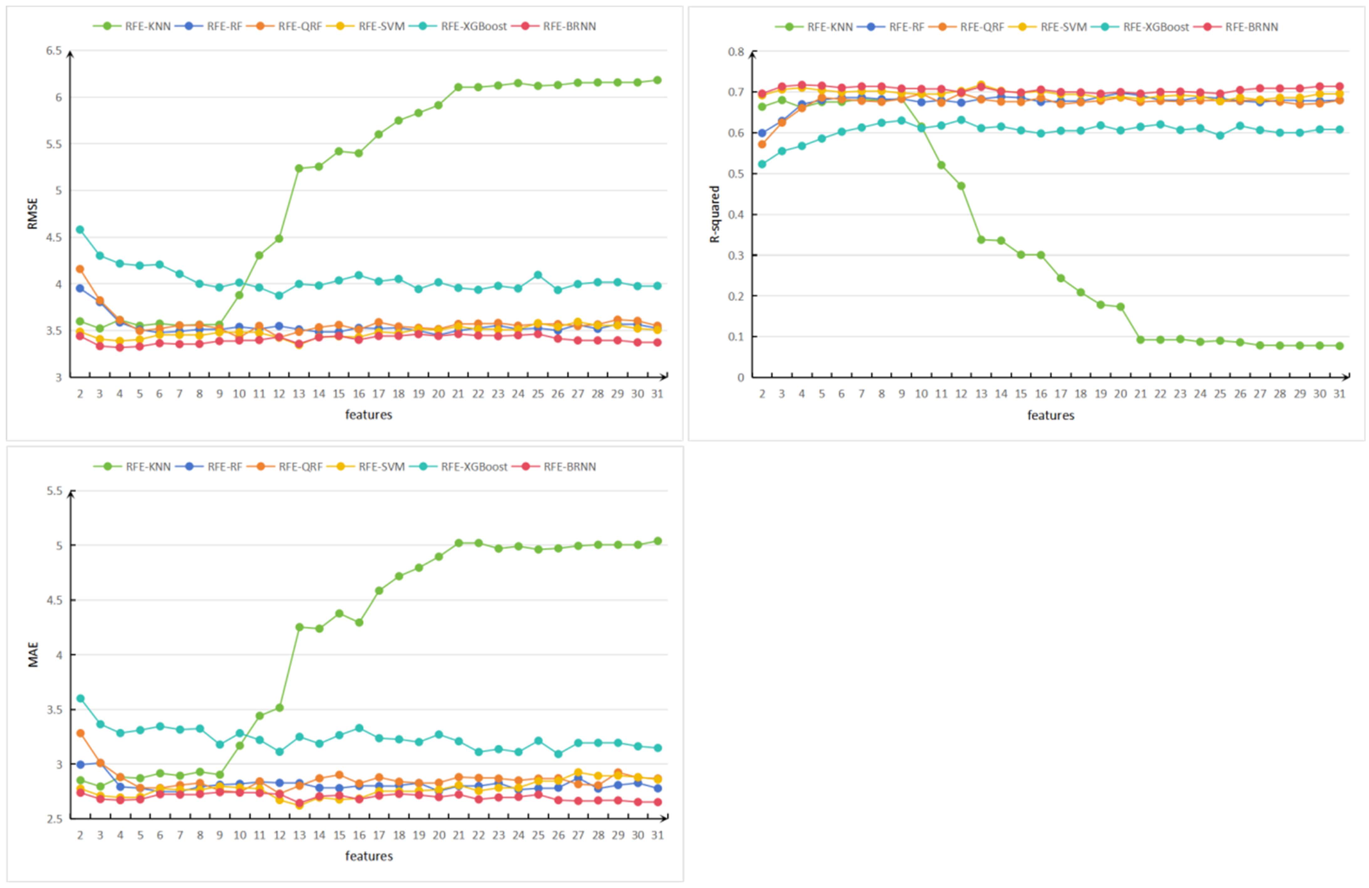
3.1.3. RFE Selection Results

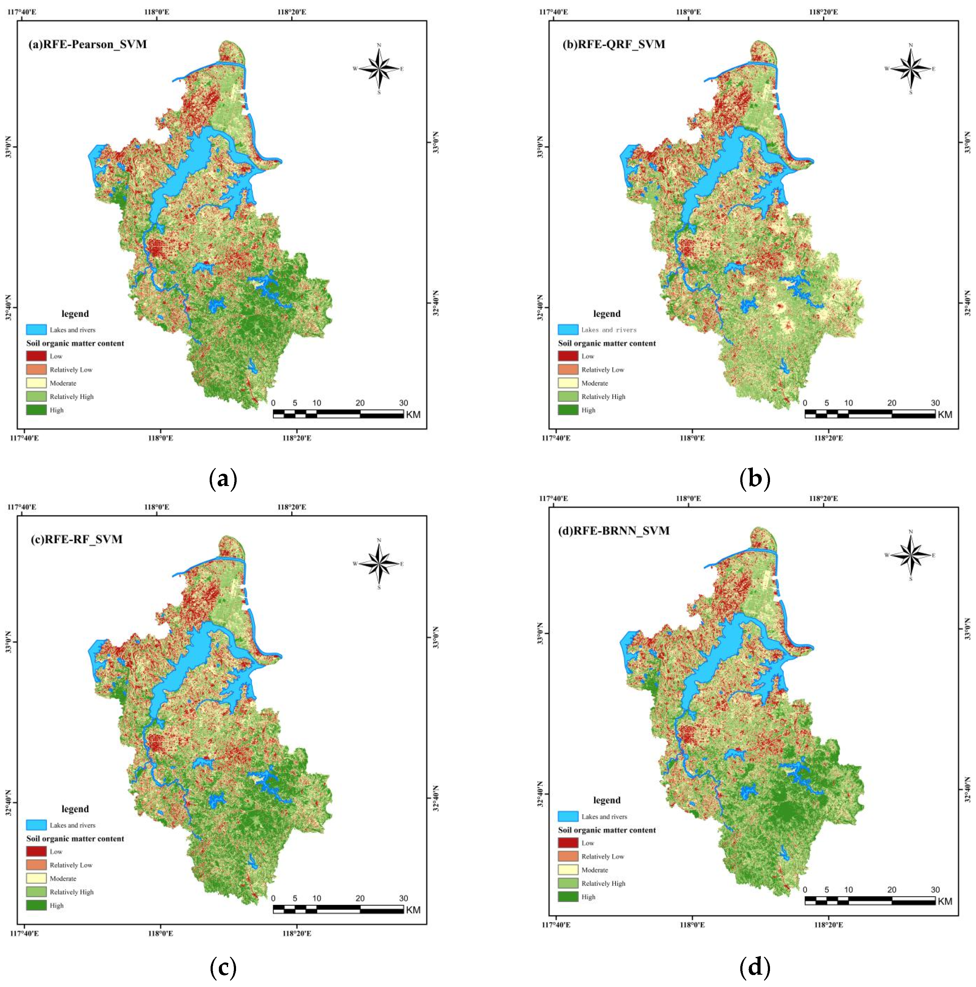
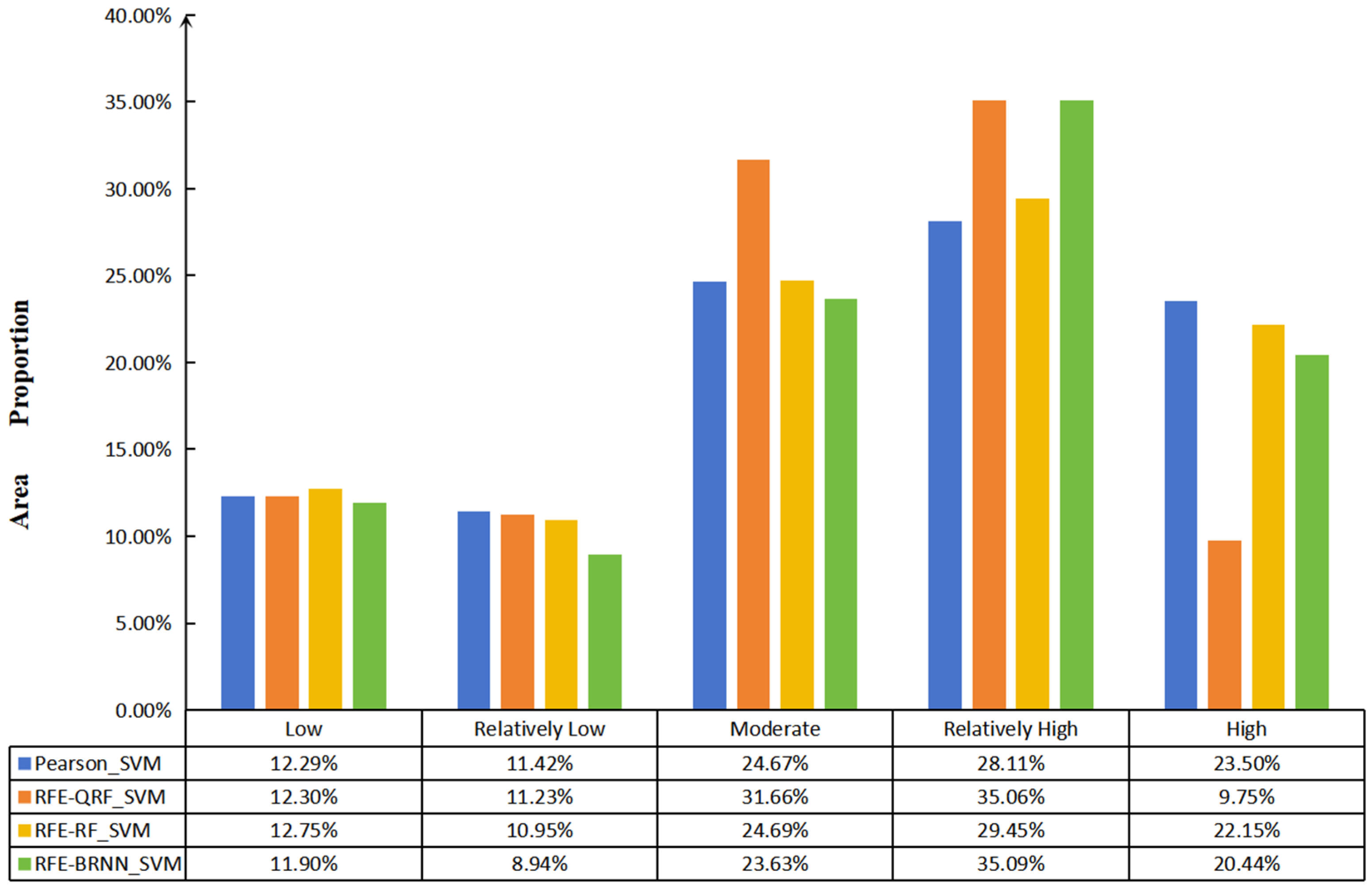
In this study, recursive feature elimination analysis models were constructed based on multiple base models (K-nearest neighbors, SVM, RF, QRF, XGBoost, and BRNN) to find multiple optimal feature subsets from a total of 31 variables. Each number of variable subsets [41,55,56] was tried, and the comparison results are shown in Figure 4. Among all the models, the recursive feature elimination model based on the BRNN algorithm had the highest accuracy (RMSE = 3.319). Compared with the results based on KNN, SVM, RF, QRF, and XGBoost algorithms, the RMSE index was lower by 0.204, 0.027, 0.134, 0.107, and 0.556, respectively. The optimal feature subset selected a total of four variables (Band_7, Band_2, Band_6, Band_1). The recursive feature elimination model based on the SVM algorithm had the best fitting effect (R-squared = 0.718). Compared with the results based on K-nearest neighbors, RF, QRF, XGBoost, and BRNN algorithms, the R-squared index was higher by 0.038, 0.021, 0.021, 0.086, and 0.001, respectively. The optimal feature subset selected a total of 13 variables (Band_7, Band_2, Band_6, Band_1, Band_3, Band_5, Band_4, DVI, Y, X, VARI, Elevation, NDVI_12). The recursive feature elimination model based on the QRF algorithm had better accuracy than XGBoost but selected the same set of feature variables.

3.2. SOM Mapping

In this study, 60 model groups were generated by combining the 10 feature variable subsets screened by 3 methods with 6 machine learning models. The optimal model was selected to generate the spatial distribution map of SOM based on indicators such as RMSE, R-squared, and VSI of the training set and test set. The data of each indicator in the 60 model groups are diverse. In the case of higher accuracy, select the top four model groups with the smallest VSI to generate four spatial distribution maps of SOM. According to the characteristics of SOM content, it is divided into five levels: high (>35 g/kg), higher (25 g/kg–35 g/kg), medium (15 g/kg–25 g/kg), lower (10 g/kg–15 g/kg), and low (<10 g/kg), as shown in Figure 5.

The proportion of each SOM content level obtained from the optimal model groups in Figure 6 shows that there is a problem of low SOM level in the study area, which is likely to occur mainly on cultivated land. It can be clearly seen from the figure that the SOM content in the whole study area is distributed from south to north with higher levels in the south and lower levels in the north. The natural surface soil in the low mountainous areas in the south has a high level of organic matter, while the central and northwestern areas are mostly hilly lands with relatively low altitude but large topographic relief. The water shortage at the top of the hills is mostly used for dry farming, and the fields between the hills are all paddy fields, resulting in a staggered distribution of SOM content in this part of the region.

The SOM level in most areas of the region is concentrated at medium and higher levels, which is related to the long-term land improvement work and soil testing and formula fertilization projects in the area, aiming to improve the overall soil fertility of the local area. In particular, the natural SOM in the forests of the low mountainous areas in the south has not been destroyed due to the decay of animals and plants. The SOM map generated by RFE-RF_SVM (Figure 5c) shows that about 12.75% of the regional area belongs to the SOM deficiency area, with lower and higher levels of SOM content accounting for 10.95% and 22.15%, respectively, and medium and higher levels being the main concentrated areas, accounting for 24.69% and 28.45%, respectively. The SOM map generated by the RFE-QRF_SVM model group (Figure 5b) shows that the high level of organic matter content area is only 9.75%, which is the smallest among the four models. The results of the RFE-BRNN_SVM model group (Figure 5d) show that the lower-level area is the smallest, accounting for only 8.94%. The overall trend of the results of the Pearson_SVM model group is highly consistent with that of the optimal model, with 12.29%, 11.42%, 24.67%, 28.11% and 23.50% under the classification standard from low to high, respectively.

The purpose of comparing and evaluating these four result maps is to understand the prediction efficiency of optimal model combination and selected feature subsets on SOM content. The RFE-QRF_SVM model group has a much lower proportion in the high level compared with other models, while it has a higher proportion in the medium and higher levels than other models. The RFE-BRNN_SVM model has a higher proportion in the higher level, resulting in a lower proportion in the lower level than other models. The Pearson_SVM and RFE-RF_SVM model groups have similar results in each level, which are superior in stability to the other two model combinations, and their VSI values are also very close. Low-level SOM content is mostly related to soil moisture, soil structure, biomass, and topography, while medium-level SOM is mostly related to land use patterns and topography. High-level is closely related to land vegetation types, altitude, and topography. Therefore, areas with large topographic relief, loose soil structure, exposed or low biomass surface coverage in the study area have relatively low organic matter content, mainly distributed in some parts of the northwest and central regions.

3.3. Performance Evaluation of Combined Models

3.3.1. Combined Model Training Accuracy

This study trained a total of 123 samples, which were divided into 9 types based on 3 feature variable screening methods, and calculated 9 groups of feature subsets, plus a total of 10 groups of feature variable sets, which were then applied to 6 machine learning models in turn. As a result, 60 model combination scenarios and their training results were obtained, as shown in

Table 2. Each model combines results on the training set and the test set.

Variable Filtering	Learning Model	Training_RMSE	Training_Q-Squared	Training_MAE	Testing-RMSE	Testing-Q-Squared	Testing-MAE
All	KNN	6.107	0.099	5.090	6.121	0.213	5.163
	SVM	3.639	0.694	3.071	3.546	0.722	2.875
	RF	3.365	0.721	2.767	3.587	0.721	2.983
	QRF	3.413	0.715	2.800	3.977	0.684	3.273
	XGBoost	3.741	0.668	2.971	3.917	0.660	3.162
	BRNN	3.377	0.723	2.765	3.674	0.701	3.129
Pearson	KNN	6.075	0.114	5.025	6.032	0.242	5.101
	SVM	3.549	0.714	2.951	3.586	0.719	2.935
	RF	3.329	0.729	2.747	3.718	0.711	3.045
	QRF	3.407	0.719	2.819	3.752	0.723	3.121
	XGBoost	3.593	0.692	2.896	3.721	0.694	3.013
	BRNN	3.384	0.726	2.775	3.709	0.695	3.108
SR	KNN	5.652	0.250	4.548	6.011	0.202	4.943
	SVM	3.105	0.771	2.535	3.494	0.732	2.900
	RF	3.392	0.711	2.757	3.774	0.693	3.104
	QRF	3.377	0.715	2.803	3.818	0.702	3.122
	XGBoost	3.423	0.694	2.718	3.893	0.665	3.175
	BRNN	3.078	0.760	2.507	3.658	0.703	3.108
SR-VIF	KNN	5.892	0.215	4.804	6.450	0.085	5.278
	SVM	6.010	0.134	4.984	6.537	0.059	5.300
	RF	5.475	0.233	4.387	5.744	0.289	4.488
	QRF	5.368	0.275	4.271	5.638	0.297	4.329
	XGBoost	5.963	0.223	4.711	6.848	0.106	5.658
	BRNN	5.892	0.133	4.840	6.513	0.064	5.318
RFE-KNN	KNN	3.437	0.708	2.844	3.488	0.734	0.940
	SVM	3.343	0.728	2.711	3.388	0.765	2.789
	RF	3.500	0.698	2.836	3.726	0.693	2.993
	QRF	3.535	0.688	2.848	3.895	0.669	3.142
	XGBoost	3.954	0.633	3.136	4.457	0.594	3.644
	BRNN	3.307	0.830	2.704	3.397	0.749	2.866
RFE-SVM	KNN	4.755	0.431	3.832	5.091	0.445	4.017
	SVM	3.278	0.755	2.622	3.517	0.730	2.894
	RF	3.323	0.723	2.716	3.464	0.745	2.839
	QRF	3.334	0.730	2.734	3.414	0.759	2.765
	XGBoost	3.545	0.691	2.878	4.087	0.630	3.324
	BRNN	3.249	0.750	2.657	3.726	0.692	3.158
RFE-RF	KNN	6.057	0.121	4.997	6.084	0.217	5.111
	SVM	3.470	0.728	2.826	3.504	0.730	2.874
	RF	3.343	0.724	2.745	3.537	0.729	2.857
	QRF	3.375	0.715	2.797	3.723	0.720	3.039
	XGBoost	3.470	0.708	2.676	3.698	0.697	2.821
	BRNN	3.324	0.730	2.691	3.585	0.716	2.985
RFE-QRF	KNN	4.825	0.414	3.862	5.068	0.449	3.986
	SVM	3.379	0.728	2.693	3.441	0.742	2.808
	RF	3.346	0.717	2.726	3.470	0.743	2.860
	QRF	3.374	0.716	2.737	3.501	0.740	2.842
	XGBoost	3.604	0.688	2.882	3.675	0.705	2.872
	BRNN	3.352	0.729	2.714	3.562	0.719	3.034
RFE-XGBoost	KNN	4.825	0.414	3.862	5.068	0.449	3.986
	SVM	3.379	0.728	2.693	3.441	0.742	2.808
	RF	3.346	0.717	2.726	3.470	0.743	2.860
	QRF	3.374	0.716	2.737	3.501	0.740	2.842
	XGBoost	3.604	0.688	2.882	3.675	0.705	2.872
	BRNN	3.352	0.729	2.714	3.562	0.719	3.034
RFE-BRNN	KNN	3.397	0.716	2.688	3.602	0.717	3.011
	SVM	3.376	0.724	2.727	3.367	0.767	2.761
	RF	3.296	0.732	2.675	3.740	0.690	2.999
	QRF	3.243	0.738	2.628	3.841	0.678	3.030
	XGBoost	3.629	0.682	2.864	4.518	0.582	3.555
	BRNN	3.313	0.730	2.709	3.395	0.748	2.865

Among them, the model combination of SR_BRNN has the smallest RMSE (3.078) and MAE (2.507), and the model combination of RFE-KNN_BRNN achieves the best fitting effect (R-squared = 0.830).

3.3.2. Test Set Accuracy

The 60 trained model combinations were run on the test set, which was a separate and randomly divided sample set that did not participate in model training. Correspondingly, 60 sets of test results were obtained, as shown in Table 2. Among them, RFE-BRNN had the smallest RMSE (3.367) and the largest R-squared (0.767), while RFE-KNN_KNN had the smallest MAE (0.940).

3.3.3. Comprehensive Performance

It is not scientific to choose the best model based solely on the accuracy of model training or testing, as it may lead to overfitting of the model, which performs well on the training set but poorly on new data sets. In this study, we comprehensively evaluated the results of RMSE, R-squared and VSI in the model test set, as shown in Table 2. The accuracy of 75% of the model combinations in the test set was between 3 and 4 for RMSE, between 0.6 and 0.8 for R-squared, and overall showed excellent predictive ability, indicating that the trained models can express the actual ground conditions in the study area. Among them, the optimal model combination RFE-RF_SVM can show high accuracy on new data sets, good fitting effect, and good stability, with values of RMSE = 3.504, VSI = 0.036 and R-squared = 0.730, respectively. That is to say, when ensuring that both the training set and the test set have better RMSE than the mean value, select the model with the smallest VSI value (Figure 7).

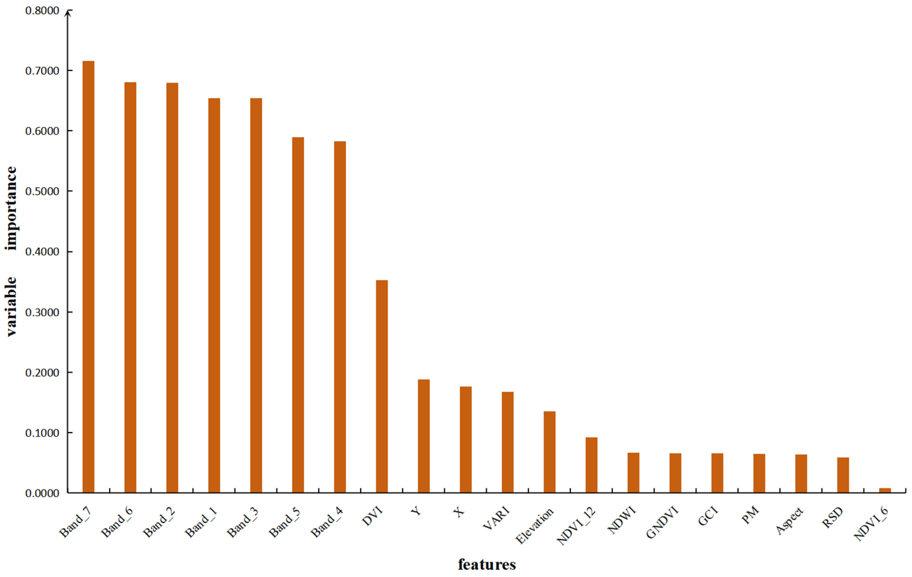
3.4. Optimal Variable Contribution Analysis

The method for selecting key feature variables in the optimal model group is based on recursive feature elimination of the random forest algorithm. By repeatedly building random forest models through backward method training, and according to the importance ranking [57], the most important feature variables are retained to form the optimal feature subset (Band_7, Band_6, Band_2, Band_3, Band_1, Band_5, Band_4, DVI, PM, Elevation, VARI, NDVI_12, Y, X, NDWI, GCI, GNDVI, RSD, Aspect, NDVI_6). The results of the optimal model group show that (Figure A1) variables such as band 7 (Band_7 = 21.96%), band 6 (Band_6 = 18.66%), band 2 (Band_2 = 10.94%), band 3 (Band_3 = 9.11%), and band 1 (Band_1 = 8.53%) have the highest contribution in this model.

Based on the optimal feature subset obtained, high-precision and high-efficiency prediction of SOM content is carried out under the model of the support vector machine algorithm. During its training process, the importance of each variable to the model is measured according to its contribution degree, and it is sorted according to its importance. Remote sensing bands have the greatest impact on model prediction. In addition, spatial variables X and Y contribute greatly, further indicating that organic matter has spatial autocorrelation. VARI, GNDVI, and GCI indicators also contribute to the prediction of SOM to a certain extent, providing new possibilities for related organic matter research, which can be further studied in depth (Figure A2).

4. Discussion

SOM plays a crucial role in soil [58]. It is not only the main source of plant nutrition, but also improves the physical properties of soil. In addition, it can enhance soil fertility and buffering, reduce pesticide residues and heavy metal hazards in soil, and promote microbial activity [59,60,61]. Accurately mastering SOM is essential for soil science research and agricultural production. Many soil scientists around the world try to use various advanced models and methods to predict and simulate accurate results. For the forecast of organic matter in deep soil layers, most depth functions are constructed to describe the change of organic matter with depth. Generally, several depth function components are defined to form a soil model [62]. The selection of models mostly compares their accuracy and fitting effect, which has the limitation of subjective judgment by researchers. In this paper, under the condition of better accuracy in the test set, the VSI index is used to clearly select the optimal model by comprehensively considering the exactness results of the model training set and test set.

This study introduces six different machine learning models and applies them to the mapping of SOM in areas with diverse terrain and landforms. The mapping results can provide good help in identifying the distribution of SOM. A new approach is proposed for mapping soil organic matter in complex terrain [63,64,65]. Among all the model groups, 70% of the model groups have good mapping accuracy, and there is little difference in their performance. However, the RFE-RF_SVM model group has better prediction and stability than other models [66,67,68]. The random forest model also has good accuracy and can be further studied in terms of feature variable screening and other aspects to find better solutions and improve the accuracy and performance of this model in predicting SOM in complex terrain areas. The mapping results generated by the optimal model group show that the SOM content in the center and northwestern regions of the study area is low, the fertility is insufficient, and there is a risk of low productivity. The main reasons for the low organic matter content in these two areas are different and vary spatially.

The top five factors for model mapping importance are landsat8 bands 7, 6, 2, 3, and 1. They all have the ability to effectively provide information on surface vegetation, material types, and soil moisture conditions, which are directly related to the source of organic matter in soil and the growth of plants and animals. These have a high correlation with organic matter [69,70,71]. The central part is dominated by hilly land, where water sources at the top of hills are scarce and mostly rely on rainfall for replenishment, restricting the survival of animals or microorganisms in the soil and resulting in low organic matter production [72]. In addition, most of the hilly land has been developed into cultivated land, with planting structures mostly consisting of wheat or rice–wheat rotations, with little tree coverage and low soil biomass [73]. Cultivated land with steeper slopes may carry away some organic matter under the action of irrigation and other running water, further affecting SOM. Most of the northwest is constrained by soil type and terrain, with more sand and gravel in the soil, large soil particles, and loose soil structure resulting in high soil porosity, which means water can easily evaporate and permeate, causing a severe loss of soil nutrients, including organic matter, with lower nutrient content [74]. Coupled with a larger terrain slope, it further promotes the loss of organic matter and other nutrients. Research found that environmental covariates VARI, GCI, and GNDVI introduced into the model had a positive effect. Among them, VARI improved the ability of soil identification and resistance to atmospheric interference [75]; GCI can measure the content of chlorophyll in various plants, reflecting the physiological state of vegetation, that is, showing the activity and abundance of vegetation growth, reflecting the level of nutrients such as organic matter from the side [76]; GNDVI can monitor the nitrogen content of vegetation, and nitrogen has a high degree of correlation and parallelism with organic matter, also expressing organic matter content to a certain extent [77]. For SOM model prediction, these vegetation indices may provide a new idea, through in-depth analysis of this vegetation index, providing a new perspective for future research.

In general, the three main sources of SOM are aboveground plant residues, root residues and root exudates, animals and microorganisms in the soil, and human-made organic fertilizer application. The connotation of environmental characteristic variables is the ability to effectively express these influencing factors. The three sources support each other and maintain SOM at a certain level. Therefore, irrigation facilities can be built to alleviate soil moisture deficiency, trees can be planted to stabilize soil and prevent water and nutrient loss, and increased organic fertilizer application can improve soil physical structure to increase SOM content [78,79]. The optimal model is obtained under the geographical spatial pattern of hills, hillocks and plains concentrated at the same time in the study area. The regional terrain is complex, but its prediction effect is unknown in other areas with larger terrain drops, such as the crisscross of mountains and plains. Further research is needed to fill this part of the missing.

5. Conclusions

This study attempts to find a set of optimal models that can accurately identify the spatial distribution of SOM in the area where Mingguang City, China is located. The model has excellent performance and accuracy, which can greatly improve the efficiency of SOM mapping, saving time and costs. Although three quarters of the 60 model groups listed in this paper have good accuracy, according to the selection of test set RMSE and VSI indicators, RFE-RF_SVM has the best comprehensive performance. It is worth noting that although the feature variable subsets obtained through various variable screening methods are different, the best models for prediction are all SVM. Therefore, it is recommended to use the support vector machine algorithm to build a prediction model under the premise of recursive feature elimination for variable screening and adjust parameters according to actual situations, which can handle the mapping problem of multi-terrain mixed areas very well. According to the results of the model, the overall level of SOM content in the center and northwestern regions of the study area is relatively low, but the causes of the lower organic matter levels in the central and northwestern parts are quite different. The model’s performance on new data sets shows that this mapping model can well understand the soil–landscape relationship and is highly consistent with the actual situation. Using digital soil mapping models based on machine learning methods can efficiently determine the spatial distribution of organic matter.

According to field sampling observations and model mapping results, the southern, central and northwestern parts of the study area face different problems. The southern part is mainly composed of low mountain areas, mostly covered by natural vegetation, with high organic matter content. However, due to human intervention, some areas have been developed into forestry farms, resulting in reduced biodiversity and hindering the accumulation of original organic matter, leading to widespread land degradation and reduced soil fertility. Due to the demand for grain cultivation, the upland areas in the central part of the study area are transformed into drylands because they are not suitable for rice cultivation. Years of continuous cultivation, lack of water resources, excessive application of chemical fertilizers, and lack of organic matter input have made the soil compact and hard. The northwestern part has loose soil structure, mostly sand and stones, but after years of cultivation, the soil quality has improved. A series of engineering projects have been implemented locally to improve the environmental conditions for SOM development, thereby improving soil quality and fertility. By drawing a spatial distribution map of SOM, we can clearly grasp the distribution of SOM in different regions, helping the government more accurately identify areas with low organic matter levels. In these areas, the government can take various measures to improve soil quality. For example, it can promote the use of organic fertilizers instead of chemical fertilizers; it can also promote the full decomposition of crop straw and return it to the field to increase the organic matter content in the soil; in addition, it can implement integrated agricultural technology that combines water and fertilizer to improve the efficiency of fertilizer use. In this way, we can more effectively improve soil quality, increase SOM levels, improve crop yields and quality, and achieve sustainable agricultural production.

References

1. Yazdanshenas, H.; Tavili, A.; Jafari, M.; Shafeian, E. Evidence for relationship between carbon storage and surface cover characteristics of soil in rangelands. Catena 2018, 167, 139–146. [Google Scholar] [CrossRef]
2. Picariello, E.; Baldantoni, D.; Izzo, F.; Langella, A.; De Nicola, F. Soil organic matter stability and microbial community in relation to different plant cover: A focus on forests characterizing Mediterranean area. Appl. Soil Ecol. 2021, 162, 103897. [Google Scholar] [CrossRef]
3. Mallah Nowkandeh, S.; Noroozi, A.A.; Homaee, M. Estimating soil organic matter content from Hyperion reflectance images using PLSR, PCR, MinR and SWR models in semi-arid regions of Iran. Environ. Dev. 2018, 25, 23–32. [Google Scholar] [CrossRef]
4. Gu, X.; Wang, Y.; Sun, Q.; Yang, G.; Zhang, C. Hyperspectral inversion of soil organic matter content in cultivated land based on wavelet transform. Comput. Electron. Agric. 2019, 167, 105053. [Google Scholar] [CrossRef]
5. Zhao, X.; Zhao, D.; Wang, J.; Triantafilis, J. Soil organic carbon (SOC) prediction in Australian sugarcane fields using Vis–NIR spectroscopy with different model setting approaches. Geoderma Reg. 2022, 30, e00566. [Google Scholar] [CrossRef]
6. Horta, A.; Azevedo, L.; Neves, J.; Soares, A.; Pozza, L. Integrating portable X-ray fluorescence (pXRF) measurement uncertainty for accurate soil contamination mapping. Geoderma 2021, 382, 114712. [Google Scholar] [CrossRef]
7. McBratney, A.B.; Santos, M.M.; Minasny, B. On digital soil mapping. Geoderma 2003, 117, 3–52. [Google Scholar] [CrossRef]
8. Dalal, R.; Henry, R. Simultaneous determination of moisture, organic carbon, and total nitrogen by near infrared reflectance spectrophotometry. Soil Sci. Soc. Am. J. 1986, 50, 120–123. [Google Scholar] [CrossRef]
9. Bond-Lamberty, B.; Hengl, T.; Mendes de Jesus, J.; Heuvelink, G.B.M.; Ruiperez Gonzalez, M.; Kilibarda, M.; Blagotić, A.; Shangguan, W.; Wright, M.N.; Geng, X.; et al. SoilGrids250m: Global gridded soil information based on machine learning. PLoS ONE 2017, 12, e0169748. [Google Scholar]
10. Zhao, D.; Arshad, M.; Wang, J.; Triantafilis, J. Soil exchangeable cations estimation using Vis-NIR spectroscopy in different depths: Effects of multiple calibration models and spiking. Comput. Electron. Agric. 2021, 182, 105990. [Google Scholar] [CrossRef]
11. Keskin, H.; Grunwald, S.; Harris, W.G. Digital mapping of soil carbon fractions with machine learning. Geoderma 2019, 339, 40–58. [Google Scholar] [CrossRef]
12. De Sousa, L.; Poggio, L.; Batjes, N.; Heuvelink, G.; Kempen, B.; Riberio, E.; Rossiter, D. SoilGrids 2.0: Producing quality-assessed soil information for the globe with quantified spatial uncertainty. Soil 2021, 7, 217–240. [Google Scholar]
13. Zeng, P.; Song, X.; Yang, H.; Wei, N.; Du, L. Digital Soil Mapping of Soil Organic Matter with Deep Learning Algorithms. ISPRS Int. J. Geo Inf. 2022, 11, 299. [Google Scholar] [CrossRef]
14. Wang, T. Research on Spatial Prediction of Soil TextureBased on GF-1 Image and Machine Learning: A Case Study of Mingguang City. Master’s Thesis, Anhui Agricultural University, Hefei, China, 2023. [Google Scholar]
15. Tobler, W.R. A computer movie simulating urban growth in the Detroit region. Econ. Geogr. 1970, 46 (Suppl. S1), 234–240. [Google Scholar] [CrossRef]
16. Sereni, L.; Guenet, B.; Lamy, I. Mapping risks associated with soil copper contamination using availability and bio-availability proxies at the European scale. Environ. Sci. Pollut. Res. 2022, 30, 19828–19844. [Google Scholar] [CrossRef] [PubMed]
17. Wanghe, K.; Guo, X.; Luan, X.; Li, K. Assessment of Urban Green Space Based on Bio-Energy Landscape Connectivity: A Case Study on Tongzhou District in Beijing, China. Sustainability 2019, 11, 4943. [Google Scholar] [CrossRef]
18. Minasny, B.; McBratney, A.B. Digital soil mapping: A brief history and some lessons. Geoderma 2016, 264, 301–311. [Google Scholar] [CrossRef]
19. Dobos, E.; Montanarella, L.; Nègre, T.; Micheli, E. A regional scale soil mapping approach using integrated AVHRR and DEM data. Int. J. Appl. Earth Obs. Geoinf. 2001, 3, 30–42. [Google Scholar] [CrossRef]
20. Grinand, C.; Arrouays, D.; Laroche, B.; Martin, M.P. Extrapolating regional soil landscapes from an existing soil map: Sampling intensity, validation procedures, and integration of spatial context. Geoderma 2008, 143, 180–190. [Google Scholar] [CrossRef]
21. Akumu, C.E.; Johnson, J.A.; Etheridge, D.; Uhlig, P.; Woods, M.; Pitt, D.G.; McMurray, S. GIS-fuzzy logic based approach in modeling soil texture: Using parts of the Clay Belt and Hornepayne region in Ontario Canada as a case study. Geoderma 2015, 239–240, 13–24. [Google Scholar] [CrossRef]
22. Sena, N.C.; Veloso, G.V.; Fernandes-Filho, E.I.; Francelino, M.R.; Schaefer, C.E.G.R. Analysis of terrain attributes in different spatial resolutions for digital soil mapping application in southeastern Brazil. Geoderma Reg. 2020, 21, e00268. [Google Scholar] [CrossRef]
23. Silveira, C.T.; Oka-Fiori, C.; Santos, L.J.C.; Sirtoli, A.E.; Silva, C.R.; Botelho, M.F. Soil prediction using artificial neural networks and topographic attributes. Geoderma 2013, 195–196, 165–172. [Google Scholar] [CrossRef]
24. Sharma, A. Integrating terrain and vegetation indices for identifying potential soil erosion risk area. Geo Spat. Inf. Sci. 2010, 13, 201–209. [Google Scholar] [CrossRef]
25. Pei, T.; Qin, C.-Z.; Zhu, A.X.; Yang, L.; Luo, M.; Li, B.; Zhou, C. Mapping soil organic matter using the topographic wetness index: A comparative study based on different flow-direction algorithms and kriging methods. Ecol. Indic. 2010, 10, 610–619. [Google Scholar] [CrossRef]
26. Heung, B.; Bulmer, C.E.; Schmidt, M.G. Predictive soil parent material mapping at a regional-scale: A Random Forest approach. Geoderma 2014, 214–215, 141–154. [Google Scholar] [CrossRef]
27. Bormann, H.; Klaassen, K. Seasonal and land use dependent variability of soil hydraulic and soil hydrological properties of two Northern German soils. Geoderma 2008, 145, 295–302. [Google Scholar] [CrossRef]
28. Rossiter, D.G.; Liu, J.; Carlisle, S.; Zhu, A.X. Can citizen science assist digital soil mapping? Geoderma 2015, 259–260, 71–80. [Google Scholar] [CrossRef]
29. Ziadat, F.M. Land suitability classification using different sources of information: Soil maps and predicted soil attributes in Jordan. Geoderma 2007, 140, 73–80. [Google Scholar] [CrossRef]
30. Hui, D.; Adhikari, K.; Hartemink, A.E.; Minasny, B.; Bou Kheir, R.; Greve, M.B.; Greve, M.H. Digital Mapping of Soil Organic Carbon Contents and Stocks in Denmark. PLoS ONE 2014, 9, e105519. [Google Scholar]
31. Mansuy, N.; Thiffault, E.; Paré, D.; Bernier, P.; Guindon, L.; Villemaire, P.; Poirier, V.; Beaudoin, A. Digital mapping of soil properties in Canadian managed forests at 250m of resolution using the k-nearest neighbor method. Geoderma 2014, 235–236, 59–73. [Google Scholar] [CrossRef]
32. Wu, W.; Li, A.-D.; He, X.-H.; Ma, R.; Liu, H.-B.; Lv, J.-K. A comparison of support vector machines, artificial neural network and classification tree for identifying soil texture classes in southwest China. Comput. Electron. Agric. 2018, 144, 86–93. [Google Scholar] [CrossRef]
33. Awad, M.; Khanna, R.; Awad, M.; Khanna, R. Support vector machines for classification. In Efficient Learning Machines: Theories, Concepts, and Applications for Engineers and System Designers; Apress: Berkeley, CA, USA, 2015; pp. 39–66. [Google Scholar]
34. Grimm, R.; Behrens, T.; Märker, M.; Elsenbeer, H. Soil organic carbon concentrations and stocks on Barro Colorado Island—Digital soil mapping using Random Forests analysis. Geoderma 2008, 146, 102–113. [Google Scholar] [CrossRef]
35. Meinshausen, N.; Ridgeway, G. Quantile regression forests. J. Mach. Learn. Res. 2006, 7, 983–999. [Google Scholar]
36. Vaysse, K.; Lagacherie, P. Using quantile regression forest to estimate uncertainty of digital soil mapping products. Geoderma 2017, 291, 55–64. [Google Scholar] [CrossRef]
37. Lu, Q.; Tian, S.; Wei, L. Digital mapping of soil pH and carbonates at the European scale using environmental variables and machine learning. Sci. Total Environ. 2023, 856, 159171. [Google Scholar] [CrossRef] [PubMed]
38. Hateffard, F.; Dolati, P.; Heidari, A.; Zolfaghari, A.A. Assessing the performance of decision tree and neural network models in mapping soil properties. J. Mt. Sci. 2019, 16, 1833–1847. [Google Scholar] [CrossRef]
39. Behrens, T.; Förster, H.; Scholten, T.; Steinrücken, U.; Spies, E.D.; Goldschmitt, M. Digital soil mapping using artificial neural networks. J. Plant Nutr. Soil Sci. 2005, 168, 21–33. [Google Scholar] [CrossRef]
40. Tien Bui, D.; Pradhan, B.; Lofman, O.; Revhaug, I.; Dick, O.B. Landslide susceptibility assessment in the Hoa Binh province of Vietnam: A comparison of the Levenberg–Marquardt and Bayesian regularized neural networks. Geomorphology 2012, 171–172, 12–29. [Google Scholar] [CrossRef]
41. Camera, C.; Zomeni, Z.; Noller, J.S.; Zissimos, A.M.; Christoforou, I.C.; Bruggeman, A. A high resolution map of soil types and physical properties for Cyprus: A digital soil mapping optimization. Geoderma 2017, 285, 35–49. [Google Scholar] [CrossRef]
42. Nabiollahi, K.; Golmohamadi, F.; Taghizadeh-Mehrjardi, R.; Kerry, R.; Davari, M. Assessing the effects of slope gradient and land use change on soil quality degradation through digital mapping of soil quality indices and soil loss rate. Geoderma 2018, 318, 16–28. [Google Scholar] [CrossRef]
43. Cohen, I.; Huang, Y.; Chen, J.; Benesty, J.; Benesty, J.; Chen, J.; Huang, Y.; Cohen, I. Pearson correlation coefficient. In Noise Reduction in Speech Processing; Springer: Berlin/Heidelberg, Germany, 2009; pp. 1–4. [Google Scholar]
44. Mondejar, J.P.; Tongco, A.F. Estimating topsoil texture fractions by digital soil mapping—A response to the long outdated soil map in the Philippines. Sustain. Environ. Res. 2019, 29, 31. [Google Scholar] [CrossRef]
45. Mosleh, Z.; Salehi, M.H.; Jafari, A.; Borujeni, I.E.; Mehnatkesh, A. The effectiveness of digital soil mapping to predict soil properties over low-relief areas. Environ. Monit. Assess. 2016, 188, 195. [Google Scholar] [CrossRef] [PubMed]
46. Hamzehpour, N.; Shafizadeh-Moghadam, H.; Valavi, R. Exploring the driving forces and digital mapping of soil organic carbon using remote sensing and soil texture. Catena 2019, 182, 104141. [Google Scholar] [CrossRef]
47. Brungard, C.W.; Boettinger, J.L.; Duniway, M.C.; Wills, S.A.; Edwards, T.C. Machine learning for predicting soil classes in three semi-arid landscapes. Geoderma 2015, 239–240, 68–83. [Google Scholar] [CrossRef]
48. Zhao, Z.-D.; Zhao, M.-S.; Lu, H.-L.; Wang, S.-H.; Lu, Y.-Y. Digital Mapping of Soil pH Based on Machine Learning Combined with Feature Selection Methods in East China. Sustainability 2023, 15, 12874. [Google Scholar] [CrossRef]
49. Piikki, K.; Söderström, M. Digital soil mapping of arable land in Sweden—Validation of performance at multiple scales. Geoderma 2019, 352, 342–350. [Google Scholar] [CrossRef]
50. Brus, D.J.; Kempen, B.; Heuvelink, G.B.M. Sampling for validation of digital soil maps. Eur. J. Soil Sci. 2011, 62, 394–407. [Google Scholar] [CrossRef]
51. Srisomkiew, S.; Kawahigashi, M.; Limtong, P. Digital mapping of soil chemical properties with limited data in the Thung Kula Ronghai region, Thailand. Geoderma 2021, 389, 114942. [Google Scholar] [CrossRef]
52. Chicco, D.; Warrens, M.J.; Jurman, G. The coefficient of determination R-squared is more informative than SMAPE, MAE, MAPE, MSE and RMSE in regression analysis evaluation. Peerj Comput. Sci. 2021, 7, e623. [Google Scholar] [CrossRef] [PubMed]
53. Schober, P.; Boer, C.; Schwarte, L.A. Correlation coefficients: Appropriate use and interpretation. Anesth. Analg. 2018, 126, 1763–1768. [Google Scholar] [CrossRef]
54. Overholser, B.R.; Sowinski, K.M. Biostatistics primer: Part 2. Nutr. Clin. Pract. 2008, 23, 76–84. [Google Scholar] [CrossRef] [PubMed]
55. Yang, R.-M.; Liu, L.-A.; Zhang, X.; He, R.-X.; Zhu, C.-M.; Zhang, Z.-Q.; Li, J.-G. The effectiveness of digital soil mapping with temporal variables in modeling soil organic carbon changes. Geoderma 2022, 405, 115407. [Google Scholar] [CrossRef]
56. Chen, S.; Richer-de-Forges, A.C.; Leatitia Mulder, V.; Martelet, G.; Loiseau, T.; Lehmann, S.; Arrouays, D. Digital mapping of the soil thickness of loess deposits over a calcareous bedrock in central France. Catena 2021, 198, 105062. [Google Scholar] [CrossRef]
57. Vaysse, K.; Lagacherie, P. Evaluating Digital Soil Mapping approaches for mapping GlobalSoilMap soil properties from legacy data in Languedoc-Roussillon (France). Geoderma Reg. 2015, 4, 20–30. [Google Scholar] [CrossRef]
58. Guo, P.-T.; Li, M.-F.; Luo, W.; Tang, Q.-F.; Liu, Z.-W.; Lin, Z.-M. Digital mapping of soil organic matter for rubber plantation at regional scale: An application of random forest plus residuals kriging approach. Geoderma 2015, 237–238, 49–59. [Google Scholar] [CrossRef]
59. Lehmann, J.; Kleber, M. The contentious nature of soil organic matter. Nature 2015, 528, 60–68. [Google Scholar] [CrossRef] [PubMed]
60. Schmidt, M.W.I.; Torn, M.S.; Abiven, S.; Dittmar, T.; Guggenberger, G.; Janssens, I.A.; Kleber, M.; Kögel-Knabner, I.; Lehmann, J.; Manning, D.A.C.; et al. Persistence of soil organic matter as an ecosystem property. Nature 2011, 478, 49–56. [Google Scholar] [CrossRef] [PubMed]
61. Tiessen, H.; Cuevas, E.; Chacon, P. The role of soil organic matter in sustaining soil fertility. Nature 1994, 371, 783–785. [Google Scholar] [CrossRef]
62. Kempen, B.; Brus, D.; Stoorvogel, J. Three-dimensional mapping of soil organic matter content using soil type–specific depth functions. Geoderma 2011, 162, 107–123. [Google Scholar] [CrossRef]
63. Rossi, G.; Ferrarini, A.; Dowgiallo, G.; Carton, A.; Gentili, R.; Tomaselli, M. Detecting complex relations among vegetation, soil and geomorphology. An in-depth method applied to a case study in the Apennines (Italy). Ecol. Complex. 2014, 17, 87–98. [Google Scholar] [CrossRef]
64. Vincent, S.; Lemercier, B.; Berthier, L.; Walter, C. Spatial disaggregation of complex Soil Map Units at the regional scale based on soil-landscape relationships. Geoderma 2018, 311, 130–142. [Google Scholar] [CrossRef]
65. Camacho, M.E.; Quesada-Román, A.; Mata, R.; Alvarado, A. Soil-geomorphology relationships of alluvial fans in Costa Rica. Geoderma Reg. 2020, 21, e00258. [Google Scholar] [CrossRef]
66. Pereira, G.W.; Valente, D.S.M.; de Queiroz, D.M.; Santos, N.T.; Fernandes-Filho, E.I. Soil mapping for precision agriculture using support vector machines combined with inverse distance weighting. Precis. Agric. 2022, 23, 1189–1204. [Google Scholar] [CrossRef]
67. Heung, B.; Ho, H.C.; Zhang, J.; Knudby, A.; Bulmer, C.E.; Schmidt, M.G. An overview and comparison of machine-learning techniques for classification purposes in digital soil mapping. Geoderma 2016, 265, 62–77. [Google Scholar] [CrossRef]
68. Nketia, K.A.; Asabere, S.B.; Ramcharan, A.; Herbold, S.; Erasmi, S.; Sauer, D. Spatio-temporal mapping of soil water storage in a semi-arid landscape of northern Ghana—A multi-tasked ensemble machine-learning approach. Geoderma 2022, 410, 115691. [Google Scholar] [CrossRef]
69. Mulder, V.L.; de Bruin, S.; Schaepman, M.E.; Mayr, T.R. The use of remote sensing in soil and terrain mapping—A review. Geoderma 2011, 162, 1–19. [Google Scholar] [CrossRef]
70. Goossens, R.; Van Ranst, E. The use of remote sensing to map gypsiferous soils in the Ismailia Province (Egypt). Geoderma 1998, 87, 47–56. [Google Scholar] [CrossRef]
71. Mahmoudabadi, E.; Karimi, A.; Haghnia, G.H.; Sepehr, A. Digital soil mapping using remote sensing indices, terrain attributes, and vegetation features in the rangelands of northeastern Iran. Environ. Monit. Assess. 2017, 189, 500. [Google Scholar] [CrossRef] [PubMed]
72. Kane, E.S.; Hockaday, W.C.; Turetsky, M.R.; Masiello, C.A.; Valentine, D.W.; Finney, B.P.; Baldock, J.A. Topographic controls on black carbon accumulation in Alaskan black spruce forest soils: Implications for organic matter dynamics. Biogeochemistry 2010, 100, 39–56. [Google Scholar] [CrossRef]
73. Du Preez, C.C.; Van Huyssteen, C.W.; Mnkeni, P.N. Land use and soil organic matter in South Africa 2: A review on the influence of arable crop production. S. Afr. J. Sci. 2011, 107, 1–8. [Google Scholar] [CrossRef]
74. Riley, H.; Pommeresche, R.; Eltun, R.; Hansen, S.; Korsaeth, A. Soil structure, organic matter and earthworm activity in a comparison of cropping systems with contrasting tillage, rotations, fertilizer levels and manure use. Agric. Ecosyst. Environ. 2008, 124, 275–284. [Google Scholar] [CrossRef]
75. Xue, J.; Su, B. Significant Remote Sensing Vegetation Indices: A Review of Developments and Applications. J. Sens. 2017, 2017, 1353691. [Google Scholar] [CrossRef]
76. Haboudane, D.; Miller, J.R.; Tremblay, N.; Zarco-Tejada, P.J.; Dextraze, L. Integrated narrow-band vegetation indices for prediction of crop chlorophyll content for application to precision agriculture. Remote Sens. Environ. 2002, 81, 416–426. [Google Scholar] [CrossRef]
77. Lu, M.-y.; Liu, Y.; Liu, G.-j. Precise prediction of soil organic matter in soils planted with a variety of crops through hybrid methods. Comput. Electron. Agric. 2022, 200, 107246. [Google Scholar] [CrossRef]
78. Sanchez, P.A.; Ahamed, S.; Carré, F.; Hartemink, A.E.; Hempel, J.; Huising, J.; Lagacherie, P.; McBratney, A.B.; McKenzie, N.J.; Mendonça-Santos, M.D.L. Digital soil map of the world. Science 2009, 325, 680–681. [Google Scholar] [CrossRef] [PubMed]
79. Brevik, E.C.; Calzolari, C.; Miller, B.A.; Pereira, P.; Kabala, C.; Baumgarten, A.; Jordán, A. Soil mapping, classification, and pedologic modeling: History and future directions. Geoderma 2016, 264, 256–274. [Google Scholar] [CrossRef]
Figure 1. Geographic location of the study area and soil sample sites(The circle and straight line in the upper left area of the figure represent the approximate range of the North-South demarcation line of China).
Sustainability 16 04312 g001
Figure 2. Methodology flow chart of this study.
Sustainability 16 04312 g002
Figure 3. Environmental factors used in the study: (a) Band_1, (b) Band_2, (c) Band_3, (d) Band_4, (e) Band_5, (f) Band_7, (g) Elevation, (h) LUS, (i) DVI, (j) ENDVI, (k) GCI, (l) GNDVI, (m) VARI, (n) Y, (o) RSD, (p) PM, (q) NDVI, (r) NDVI_12, (s) NDWI, (t) OSAVI, (u) WSD, (v) TWI, (w) X, (x) Band_6, (y) PLC, (z) EVI, (aa) PRC, (ab) MSAVI, (ac) Aspect, (ad) Slope, and (ae) SPI.
Sustainability 16 04312 g003
Figure 4. Various screening model accuracy results (RMSE, R-squared, MAE).
Sustainability 16 04312 g004
Figure 5. Spatial distribution map of SOM in different optimal model groups: (a) RFE-Pearson_SVM, (b) RFE-QRF_SVM, (c) RFE-RF_SVM, and (d) RFE-BRNN_SVM.
Sustainability 16 04312 g005
Figure 6. Proportion of SOM content levels in different optimal models.
Sustainability 16 04312 g006
Figure 7. VSI indicators of each model.
Sustainability 16 04312 g007