
Determinants of Yearly CO2 Emission Fluctuations: A Machine Learning Perspective to Unveil Dynamics


Abstract
1. Introduction
- Over time, how have economic factors, CO2-related industries, educational levels and population dynamics interacted to influence the short-term change in the trend of CO2 emissions across diverse countries with diverse characteristics, with respect to the factors mentioned?
- What insight in terms of the identification and quantification of the temporal dynamics and the influence of these factors can machine learning techniques highlight to deepen one’s understanding of this change over time on a global scale?
2. Materials and Methods
2.1. Data Collection
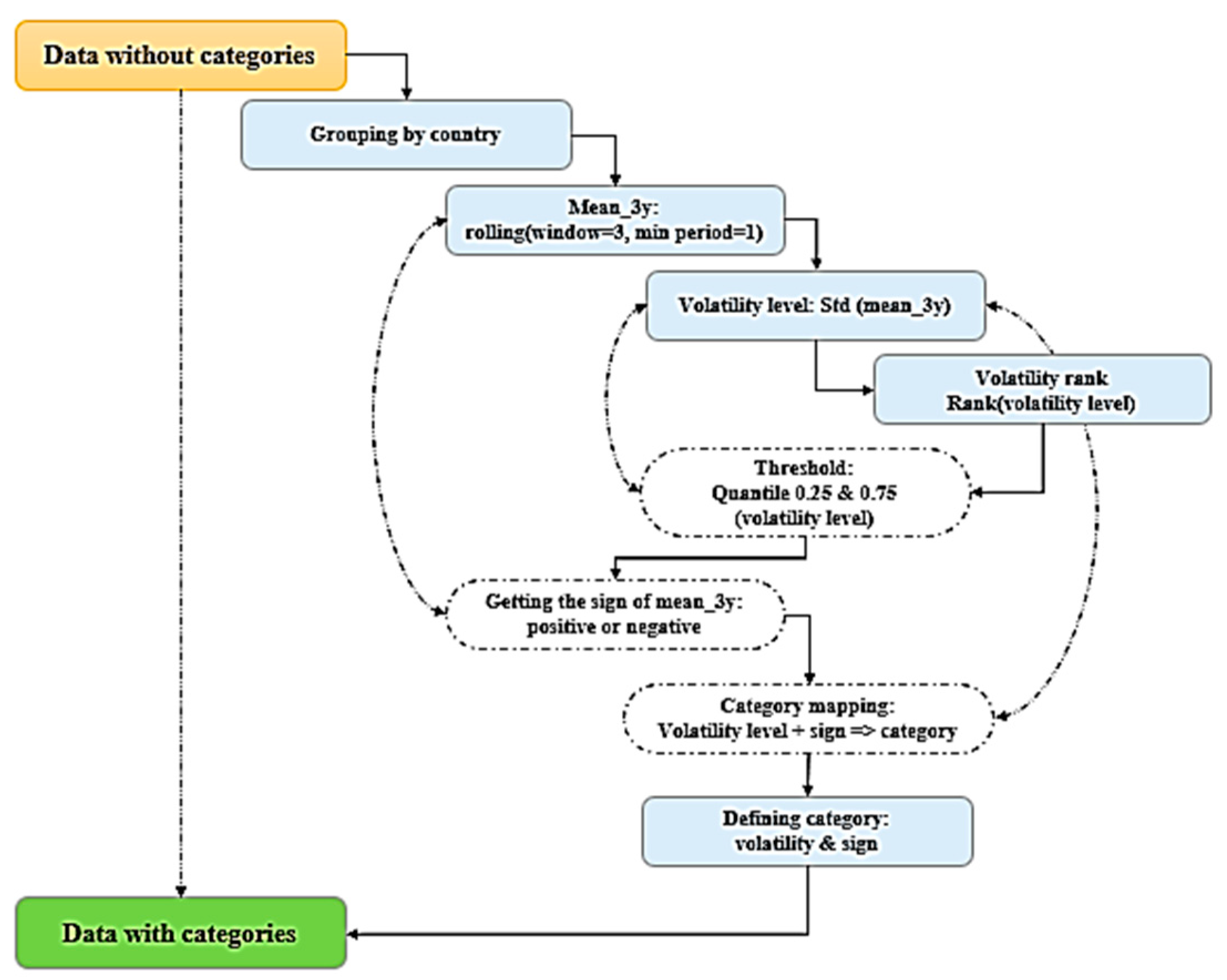
2.2. Data Preparation
2.3. Machine Learning Algorithms
2.4. Metrics
- o
- For the selection of the best performing algorithm:
- o
- For final evaluation:
- ▪
- Regression: Mean squared error, Residuals, R-squared
- ▪
- Classification: Accuracy score, Matthew correlation coefficient [33], Confusion matrix and classification report.
2.5. Explainable Machine Learning Techniques
2.5.1. Partial Dependence Plots (PDPs)
2.5.2. Sensitivity Analysis
2.5.3. Feature Analysis
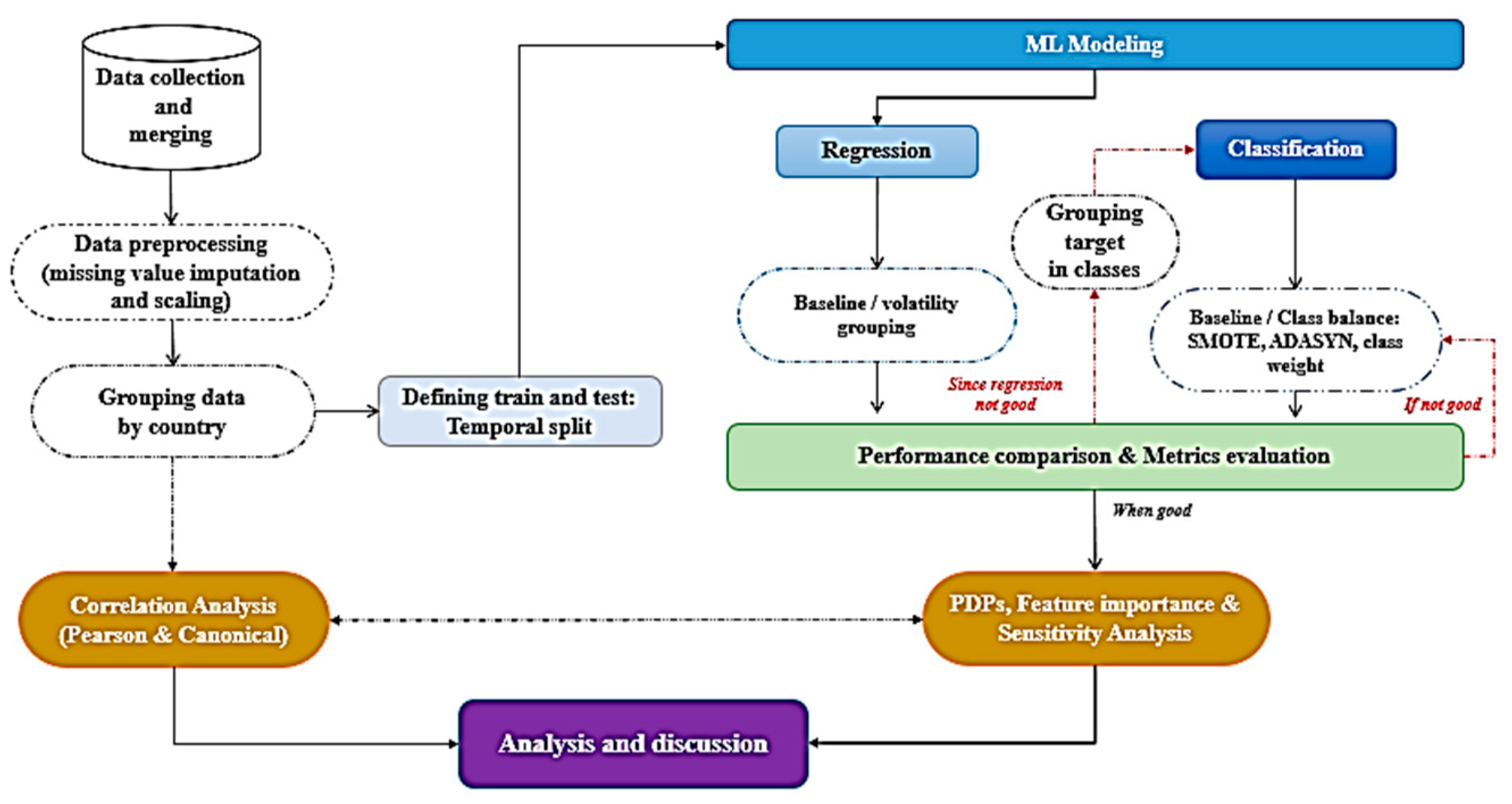
2.6. Research Design
3. Results
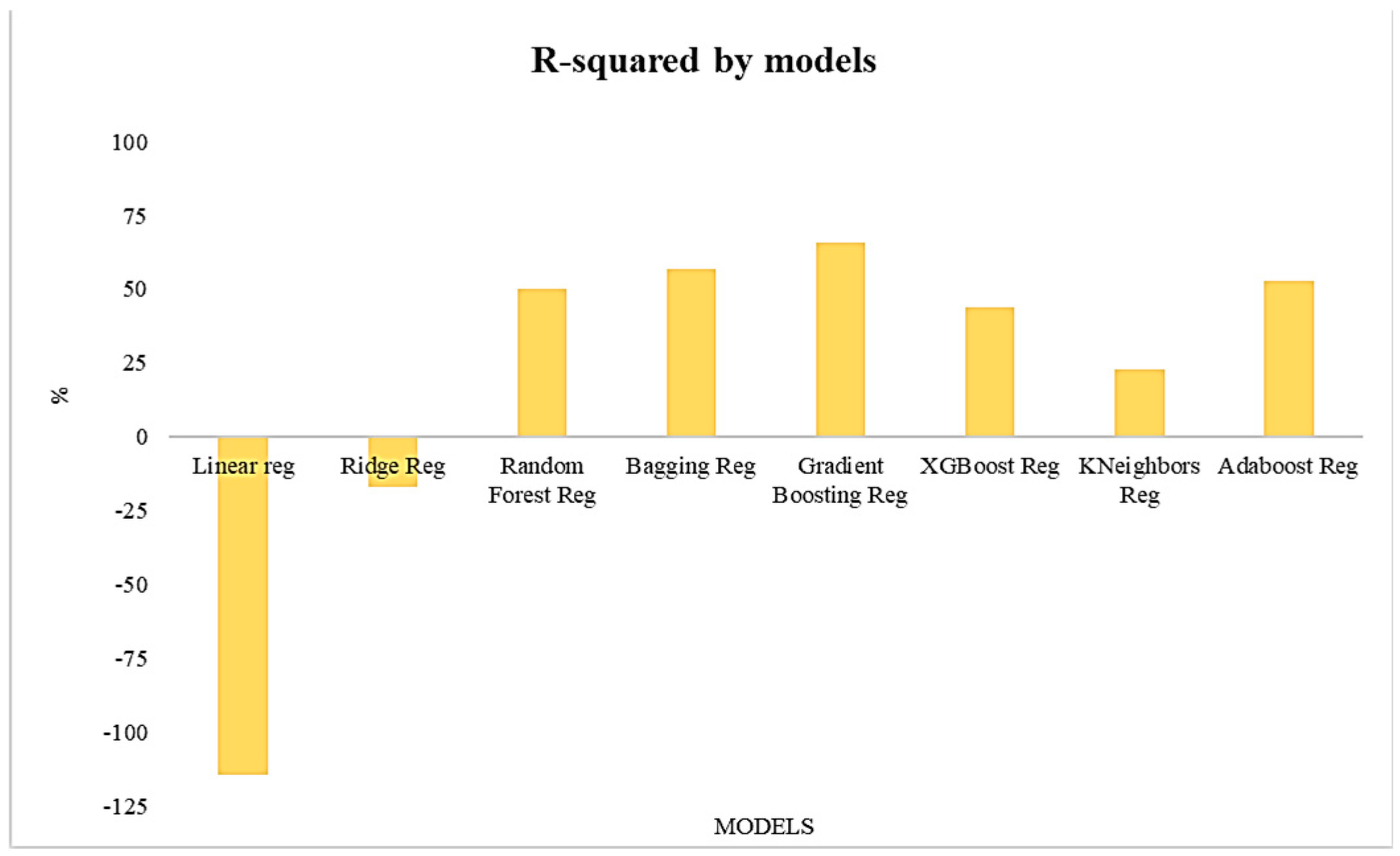
3.1. Regression Analysis
3.2. Classification Analysis
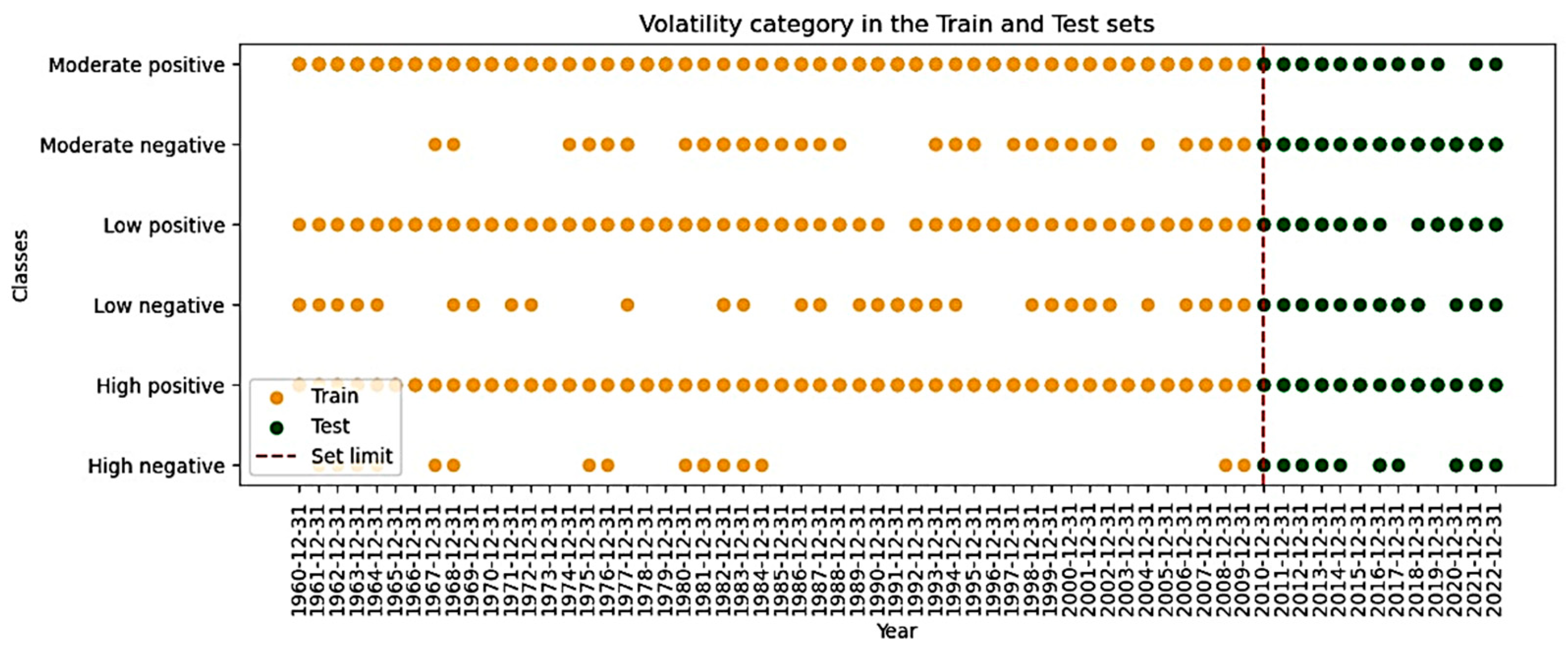
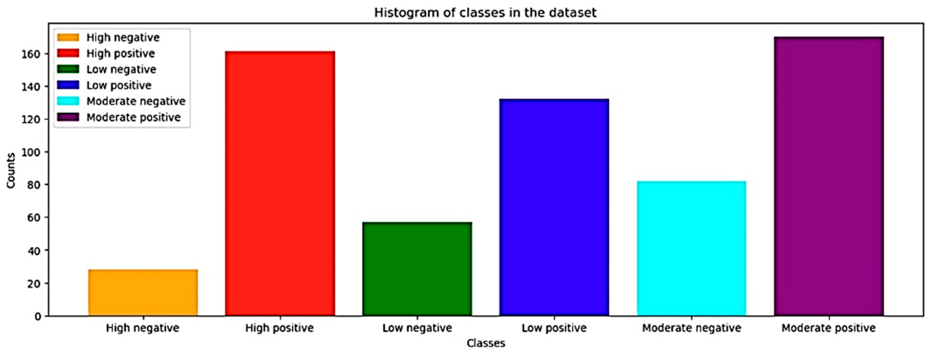
Grouping Target in Classes
3.3. Feature Analysis
3.3.1. Feature Importance Analysis
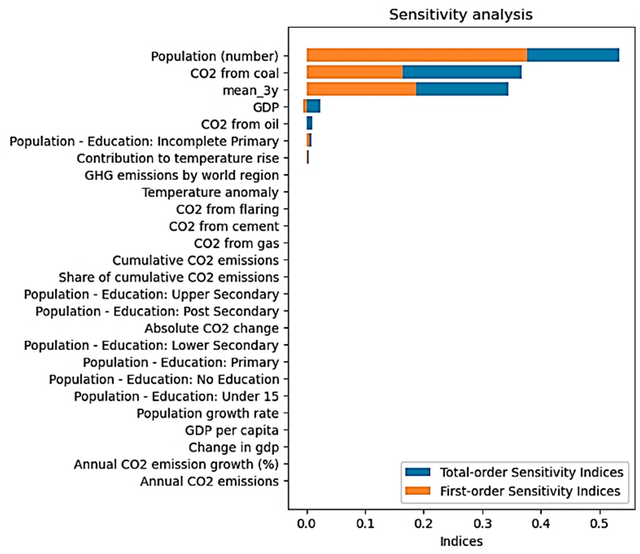
3.3.2. Sensitivity Analysis
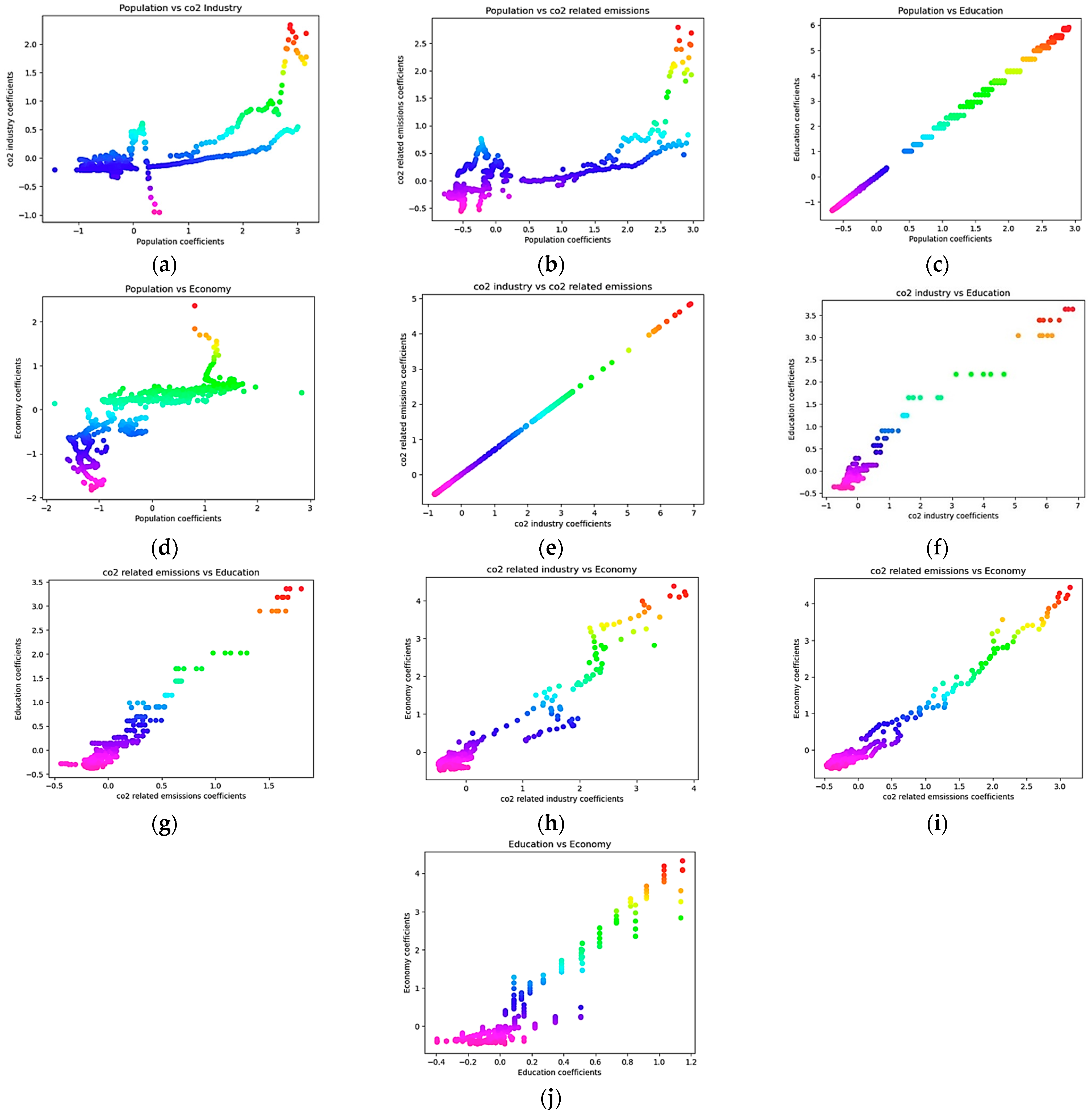
3.3.3. Correlation Analysis
3.4. Discussion
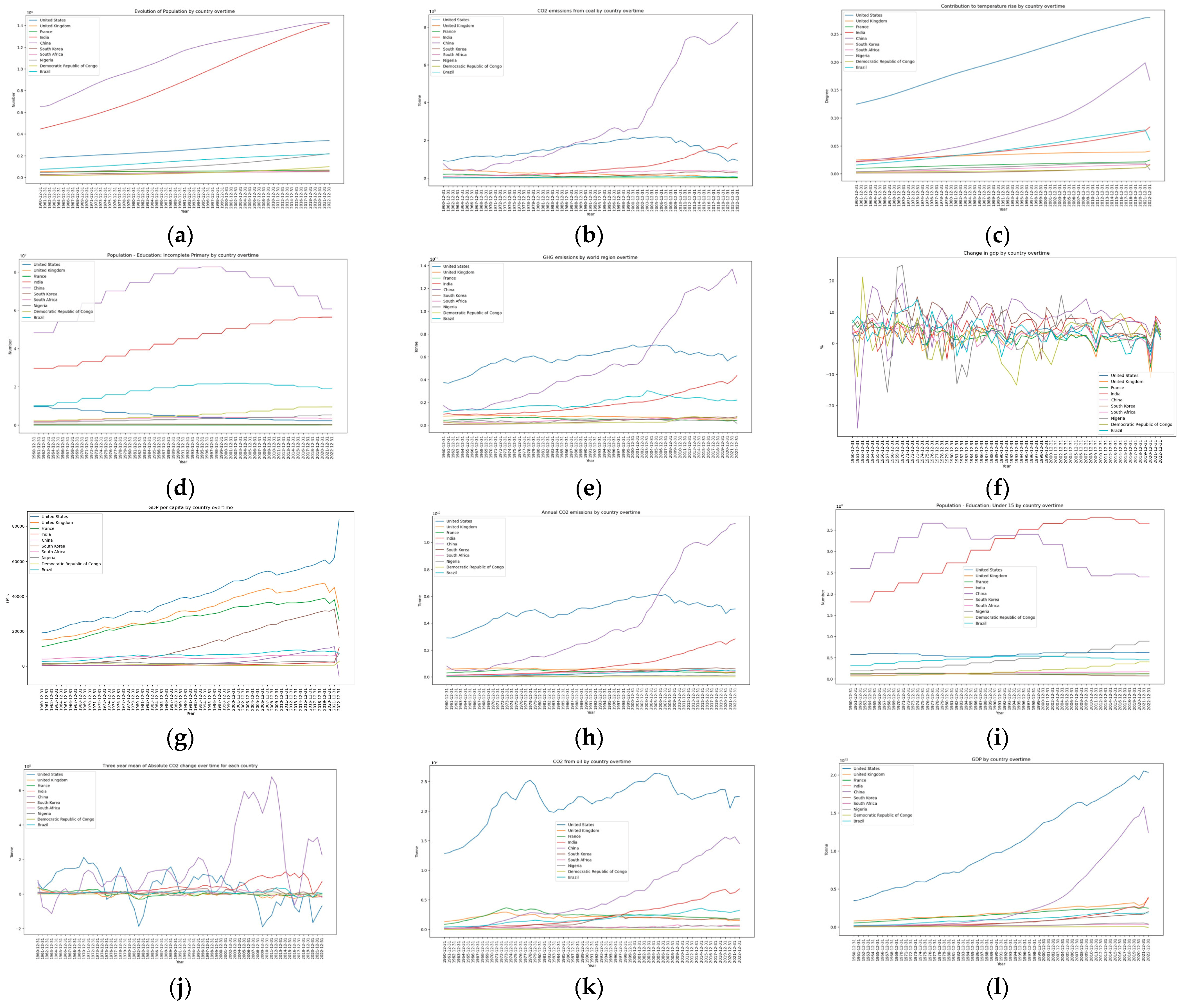
- High negative: Countries in this group have a high average population and GDP, a high CO2 emission from both coal and oil. Despite their high GDP and CO2 emissions, these countries have seen a decrease in CO2 emissions over time. However, they also have a high contribution to temperature rise. These countries’ high contribution to global warming is due to their extensive use of fossil fuels for energy production, industrial processes, and transportation. Despite recent decreases in emissions, the cumulative effect of their past and present emissions continues to drive global temperature rise.
- High positive: Countries in this group also have a high average population, a slightly lower GDP compared to the High negative group, and they have seen an increase in CO2 emissions over time. Surprisingly, they have a lower contribution to temperature rise compared to the High negative group. This could be due to their past contribution.
- Low negative: Countries in this group have a lower average population and GDP compared to the High groups. They have lower CO2 emissions from both coal and oil and have seen a decrease in CO2 emissions over time. Finally, they contribute less to temperature rise compared to the High groups.
- Low positive: Countries in this group have a similar average population to the Low negative group. They have a lower GDP compared to the Low negative group but they have seen an increase in CO2 emissions over time. They also contribute less to temperature rise compared to the High groups.
- Moderate negative: Countries in this group have a moderate average population and GDP. They have moderate CO2 emissions from both coal and oil, and they have seen a decrease in CO2 emissions over time. They contributed moderately to temperature rise compared to the High groups.
- Moderate positive: Countries in this group have a similar average population to the Moderate negative group. They have a lower GDP compared to the Moderate negative group and they have seen an increase in CO2 emissions over time. They have a lower contribution to temperature rise compared to the Moderate negative group.
- Population (number): The average population is higher in the High positive group (approximately 807 million) compared to the High negative group (approximately 481 million). This suggests that countries with larger populations tend to have increasing CO2 emissions.
- CO2 emissions from Coal: Both groups have high CO2 emissions from coal, but the High positive group has slightly higher emissions on average (approximately 1.76 billion tonnes) compared to the High negative group (approximately 1.45 billion tonnes).
- CO2 emissions from Oil: The High negative group has higher CO2 emissions from oil (approximately 1.58 billion tonnes) compared to the High positive group (approximately 885 million tonnes).
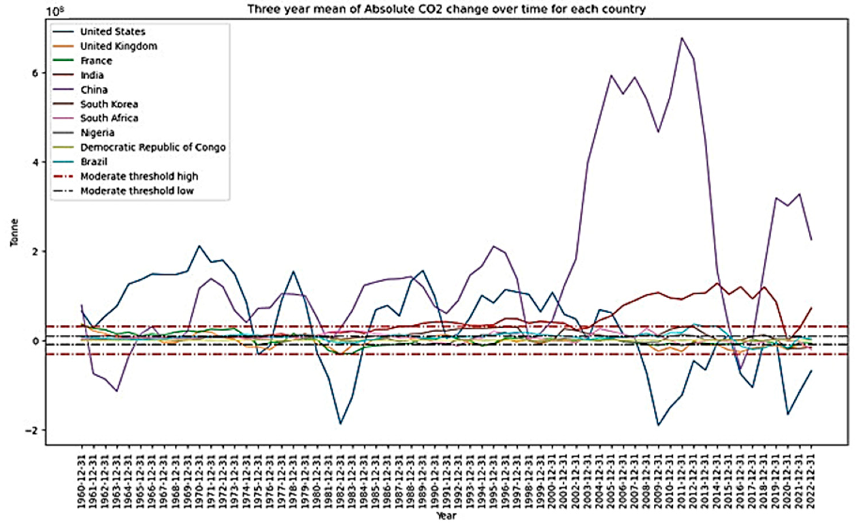
- 3-Year Mean Change in CO2 emissions (Mean-3y): The High negative group shows a decrease in CO2 emissions over time (average change of −73 million tonnes), while the High positive group shows an increase (average change of 107 million tonnes).
- GDP: is higher on average in the High negative group (approximately 9.99 trillion USD) compared to the High positive group (approximately 4.27 trillion USD). This suggests that wealthier countries tend to have decreasing CO2 emissions.
- Population with Incomplete Primary Education: The High positive group has a higher average population with incomplete primary education (approximately 43.2 million) compared to the High negative group (approximately 20.4 million).
- Contribution to Temperature Rise: The High negative group has a higher average contribution to temperature rise (0.173) compared to the High positive group (0.099).
- Population: The average population is approximately the same in both groups (approximately 67 million). This suggests that population size does not significantly differentiate these two groups.
- CO2 emissions from Coal: The Low negative group has slightly higher CO2 emissions from coal on average (approximately 104 million tonnes) compared to the Low positive group (approximately 82 million tonnes).
- 3-Year Mean Change in CO2 emissions (Mean-3y): The Low negative group shows a decrease in CO2 emissions over time (average change of −3 million tonnes), while the Low positive group shows an increase (average change of 4.8 million tonnes).
- GDP: The GDP is slightly higher on average in the Low negative group (approximately 171 billion USD) compared to the Low positive group (approximately 138 billion USD).
- CO2 emissions from Oil: The Low negative group has slightly higher CO2 emissions from oil (approximately 24 million tonnes) compared to the Low positive group (approximately 23 million tonnes).
- Population with Incomplete Primary Education: The Low positive group has a slightly higher average population with incomplete primary education (approximately 3.94 million) compared to the Low negative group (approximately 3.90 million).
- Contribution to Temperature Rise: The Low negative group has a slightly higher average contribution to temperature rise (0.0102) compared to the Low positive group (0.0085).
- Population: The average population is slightly higher in the Moderate positive group (approximately 79 million) compared to the Moderate negative group (approximately 72 million).
- CO2 emissions from Coal: The Moderate positive group has slightly higher CO2 emissions from coal on average (approximately 124 million tonnes) compared to the Moderate negative group (approximately 115 million tonnes).
- 3-Year Mean Change in CO2 emissions (Mean-3y): The Moderate negative group shows a decrease in CO2 emissions over time (average change of −10.7 million tonnes), while the Moderate positive group shows an increase (average change of 10.6 million tonnes).
- GDP: The GDP is significantly higher on average in the Moderate negative group (approximately 1.96 trillion USD) compared to the Moderate positive group (approximately 979 billion USD).
- CO2 Emissions from Oil: The Moderate negative group has higher CO2 emissions from oil (approximately 212 million tonnes) compared to the Moderate positive group (approximately 171 million tonnes).
- Population with Incomplete Primary Education: The Moderate positive group has a higher average population with incomplete primary education (approximately 5.82 million) compared to the Moderate negative group (approximately 2.10 million).
- Contribution to Temperature Rise: The Moderate negative group has a higher average contribution to temperature rise (0.029) compared to the Moderate positive group (0.0225).
4. Conclusions
Author Contributions
Funding
Institutional Review Board Statement
Informed Consent Statement
Data Availability Statement
Acknowledgments
Conflicts of Interest
Appendix A. Features Description and Rationale
| N° | Variables | Source | Unit | Description | Rationale | Source | Period Considered |
| 1 | Year-on-year change in CO2 emissions | [42] | Tonnes | Absolute annual change in carbon dioxide emissions | Target of the analysis | Global Carbon Budget, 2023) | 1960 to 2022 |
| 2 | Annual greenhouse gas emissions by world region | [43] | Tonnes | Emissions, cumulative emissions and the global mean surface temperature response by country, gas (CO2, Ch4, N2 O or GHG) and source emissions (fossil, land use) | Regional greenhouse gas emission will certainly affect the neighboring countries level of CO2 emissions | [44] | 1960 to 2021 |
| 3 | Annual temperature anomalies | [45] | Celsius | The deviation of a specific month’s average surface temperature | Fluctuations of the temperature can be informative regarding the change in CO2 emissions | [46] | 1960 to 2023 |
| 4 | Annual emissions of carbon dioxide (CO₂) from flaring | [47] | Tonnes | Annual emissions of carbon dioxide (CO₂) from flaring based on territorial emissions (excluding traded goods and international aviation) | The amount of excess of oil or gas burned during their production can explain changes in CO2 emissions | [48] | 1960 to 2022 |
| 5 | Annual emissions of carbon dioxide (CO₂) from cement | [47] | Tonnes | Annual emissions of carbon dioxide (CO₂) from cements based on territorial emissions (excluding traded goods and international aviation) | The production of concrete is an important source of CO2 emissions | [49] | 1960 to 2022 |
| 6 | Annual emissions of carbon dioxide (CO₂) from gas | [47] | Tonnes | Annual emissions of carbon dioxide (CO₂) from gas based on territorial emissions (excluding traded goods and international aviation) | The production of gas releases a significant amount of CO2 | [8,48] | 1960 to 2022 |
| 7 | Annual emissions of carbon dioxide (CO₂) from oil | [47] | Tonnes | Annual emissions of carbon dioxide (CO₂) from oil based on territorial emissions (excluding traded goods and international aviation) | The production of oil is directly linked to CO2 emissions, thus, affecting its change | [8,48] | 1960 to 2022 |
| 8 | Annual emissions of carbon dioxide (CO₂) from coal | [47] | Tonnes | Annual emissions of carbon dioxide (CO₂) from coal based on territorial emissions (excluding traded goods and international aviation) | The production of coal represents a major source of CO2 emissions | [8] | 1960 to 2022 |
| 9 | Cumulative CO2 emissions | [50] | Tonnes | Sum of CO2 emissions produced from fossil fuels and industry | The total amount of CO2 emissions accumulated during a period can significantly affect the change in CO2 emissions in a yearly period | [51] | 1960 to 2022 |
| 10 | Annual CO2 emissions growth | [50] | Percentage | Annual percentage growth of total emissions of CO2 excluding land use usage | CO2 emissions growth is an important indicator to explain changes in CO2 emissions | [8] | 1960 to 2022 |
| 11 | Share of Cumulative CO2 emissions | [52] | Tonnes | Cumulative CO2 emissions measured as a percentage of global total cumulative emissions of CO2 | Understanding which country contributes the most is an important indicator of change in CO2 emissions. | [53] | 1960 to 2022 |
| 12 | Contribution to the global mean surface temperature rise | [54] | Celsius | Each country’s contribution to global surface mean temperature rise from cumulative CO2, Ch4, N2O | This factor can indirectly explain variations of CO2 emissions | [55] | 1960 to 2021 |
| 13 | Population growth rate | [56] | Percentage | Average exponential growth of the population over a given period | The increased concentration in population generally results in many activities like urbanization, deforestation, etc., which have the potential to influence the level of CO2 emissions | [8,57] | 1960 to 2021 |
| 14 | Population (number) | [58] | Number | Population by country | Idem | [8,57] | 1960 to 2022 |
| 15 | Population with no education | [59] | Number | Educational attainment | Education plays a significant role in reducing the vulnerability of a society, and can increase awareness to pollution | [60] | 1960 to 2022 |
| 16 | Population with primary education | [59] | Number | Educational attainment | Idem | Idem | 1960 to 2022 |
| 17 | Population with incomplete primary education | [59] | Number | Educational attainment | Idem | Idem | 1960 to 2022 |
| 18 | Population with Secondary education | [59] | Number | Educational attainment | Idem | Idem | 1960 to 2022 |
| 19 | Population with upper secondary education | [58] | Number | Educational attainment | Idem | Idem | 1960 to 2022 |
| 20 | Population with lower secondary education | [59] | Number | Educational attainment | Idem | Idem | 1960 to 2022 |
| 21 | Population under 15 | [59] | Number | Educational attainment | Idem | Idem | 1960 to 2022 |
| 22 | Global Domestic Product (GDP) | [61] | US dollar | Sum of gross value added by all resident producers in the economy plus any product taxes and minus any subsidies not included in the value of the products | There is a certain correlation between the prosperity of country and its level of CO2 emissions. | 1960 to 2022 | |
| 23 | Global Domestic Product per capita | [62] | US dollar | GDP divided by midyear population | Idem | [12,63] | 1960 to 2022 |
| 24 | Change in GDP | [64] | Percentage | Annual percentage growth of GDP at market prices based on constant local currency. | Idem | [12,63] | 1960 to 2022 |
Appendix B. Statistic Description of the Dataset
| Annual CO2 Emissions | GHG Emissions by World Region | Temperature Anomaly | CO2 from Flaring | CO2 from Cement | CO2 from Gas | CO2 from Oil | CO2 from Coal | Cumulative CO2 Emissions | |
| count | 630.00 | 630.00 | 630.00 | 630.00 | 630.00 | 630.00 | 630.00 | 630.00 | 630.00 |
| mean | 1,180,717,000.00 | 1,804,513,000.00 | 0.29 | 7,744,875.00 | 39,100,780.00 | 155,176,800.00 | 377,323,700.00 | 590,266,200.00 | 49,326,940,000.00 |
| std | 2,067,422,000.00 | 2,450,693,000.00 | 0.34 | 13,920,800.00 | 120,124,900.00 | 346,134,300.00 | 645,444,900.00 | 1,255,671,000.00 | 86,020,780,000.00 |
| min | 1,647,474.00 | 51,732,420.00 | −0.31 | 0.00 | 50,771.00 | 0.00 | 688,832.00 | 0.00 | 33,411,650.00 |
| 25% | 119,760,600.00 | 428,377,400.00 | −0.02 | 0.00 | 3,499,390.00 | 493,724.80 | 34,982,420.00 | 21,795,300.00 | 2,533,510,000.00 |
| 50% | 394,471,300.00 | 669,718,000.00 | 0.25 | 2,121,456.00 | 8,233,956.00 | 19,968,290.00 | 165,657,100.00 | 135,809,200.00 | 13,698,860,000.00 |
| 75% | 634,479,800.00 | 2,143,402,000.00 | 0.58 | 6,483,802.00 | 24,980,980.00 | 90,109,130.00 | 268,966,300.00 | 416,902,800.00 | 51,740,210,000.00 |
| max | 11,396,780,000.00 | 13,710,640,000.00 | 0.93 | 88,436,970.00 | 858,232,600.00 | 1,743,539,000.00 | 2,642,692,000.00 | 8,250,736,000.00 | 426,914,600,000.00 |
| Share of Cumulative CO2 Emissions | Contribution to Temperature Rise | Population—Education: Post Secondary | Population—Education: Upper Secondary | Population—Education: Lower Secondary | Population—Education: Primary | Population—Education: Incomplete Primary | Population—Education: No Education | Population—Education: under 15 | Population (Number) | |
| count | 630.00 | 630.00 | 630.00 | 630.00 | 630.00 | 630.00 | 630.00 | 630.00 | 630.00 | 630.00 |
| mean | 5.33 | 0.05 | 16,722,340.00 | 36,436,890.00 | 43,712,180.00 | 32,234,490.00 | 14,956,620.00 | 42,991,600.00 | 82,316,990.00 | 277,365,400.00 |
| std | 9.27 | 0.06 | 27,933,400.00 | 53,308,720.00 | 97,421,520.00 | 52,721,110.00 | 22,983,330.00 | 79,366,320.00 | 115,380,700.00 | 395,267,600.00 |
| min | 0.01 | 0.00 | 36,100.00 | 68,500.00 | 430,700.00 | 0.00 | 0.00 | 0.00 | 6,612,300.00 | 15,276,560.00 |
| 25% | 0.27 | 0.01 | 1,326,700.00 | 4,598,100.00 | 5,399,125.00 | 3,810,300.00 | 444,000.00 | 2,542,500.00 | 11,825,100.00 | 50,089,850.00 |
| 50% | 1.16 | 0.02 | 5,783,600.00 | 13,641,200.00 | 10,568,000.00 | 10,126,800.00 | 3,799,500.00 | 5,732,150.00 | 25,066,800.00 | 66,412,130.00 |
| 75% | 4.75 | 0.05 | 15,051,400.00 | 39,150,200.00 | 28,268,300.00 | 27,610,400.00 | 19,467,000.00 | 30,892,300.00 | 61,191,000.00 | 250,691,100.00 |
| max | 38.78 | 0.28 | 154,720,400.00 | 250,631,200.00 | 537,276,300.00 | 200,622,500.00 | 82,623,900.00 | 292,338,700.00 | 380,274,300.00 | 1,425,894,000.00 |
| Population Growth Rate | GDP | GDP Per Capita | Change in GDP | Annual CO2 Emission Growth (%) | Absolute CO2 Change | |
| count | 630.00 | 630.00 | 630.00 | 630.00 | 630.00 | 630.00 |
| mean | 1.57 | 2,098,799,000,000.00 | 12,938.54 | 4.02 | 3.43 | 26,837,800.00 |
| std | 0.98 | 3,839,755,000,000.00 | 15,577.38 | 4.81 | 10.74 | 103,135,300.00 |
| min | −0.39 | −71,767,060,000.00 | −6173.54 | −27.27 | −48.33 | −547,516,900.00 |
| 25% | 0.68 | 166,345,200,000.00 | 1367.95 | 1.74 | −1.09 | −961,013.50 |
| 50% | 1.37 | 693,487,400,000.00 | 5221.58 | 3.85 | 3.07 | 5,909,344.00 |
| 75% | 2.45 | 1,841,303,000,000.00 | 23,704.80 | 6.73 | 6.84 | 24,604,410.00 |
| max | 5.92 | 20,529,460,000,000.00 | 83,951.61 | 25.01 | 82.62 | 911,781,900.00 |
Appendix C. Regression Results Summary
| Models | Residuals | Mean Squared Error | R-Squared | Mean Cross Validation Score | ||||||||
| Baseline | PCA | FS | Baseline | PCA | FS | Baseline | PCA | FS | Baseline | PCA | FS | |
| Linear regression | −59,327,819.08 | - | - | 3.103195 × 10²⁰ | - | - | −1.144 | - | - | −253.80 | - | - |
| Ridge Regression | −40,263,611.43 | - | - | 1.699994 × 10²⁰ | - | - | −0.17 | - | - | −29.06 | - | - |
| Random Forest Regressor | −24,435,046.47 | - | - | 59,685,956 × 108 | - | - | 0.58 | - | - | −0.89 | - | - |
| Bagging Regressor | −22,162,025.93 | - | - | 59,739,629 × 108 | - | - | 0.58 | - | - | −40.29 | - | - |
| Gradient Boosting Regressor | −14,687,525.64 | −20,216,617.8 | −18,239,234.8 | 50,060,367 × 108 | 609,461 × 106 | 4,886,957 × 105 | 0.65 | 0.57 | 0.66 | −1.88 | −0.71 | −0.71 |
| XGBoost Regressor | −28,289,899.56 | - | - | 79,866,357 × 108 | - | - | 0.44 | - | - | −53.54 | - | - |
| KNeighbors Regressor | −34,832,710.33 | - | - | 1.110808 × 10²⁰ | - | - | 0.23 | - | - | −0.32 | - | - |
| Adaboost Regressor | −23,440,275.88 | - | - | 64,210,504 × 108 | - | - | 0.55 | - | - | −1.24 | - | - |
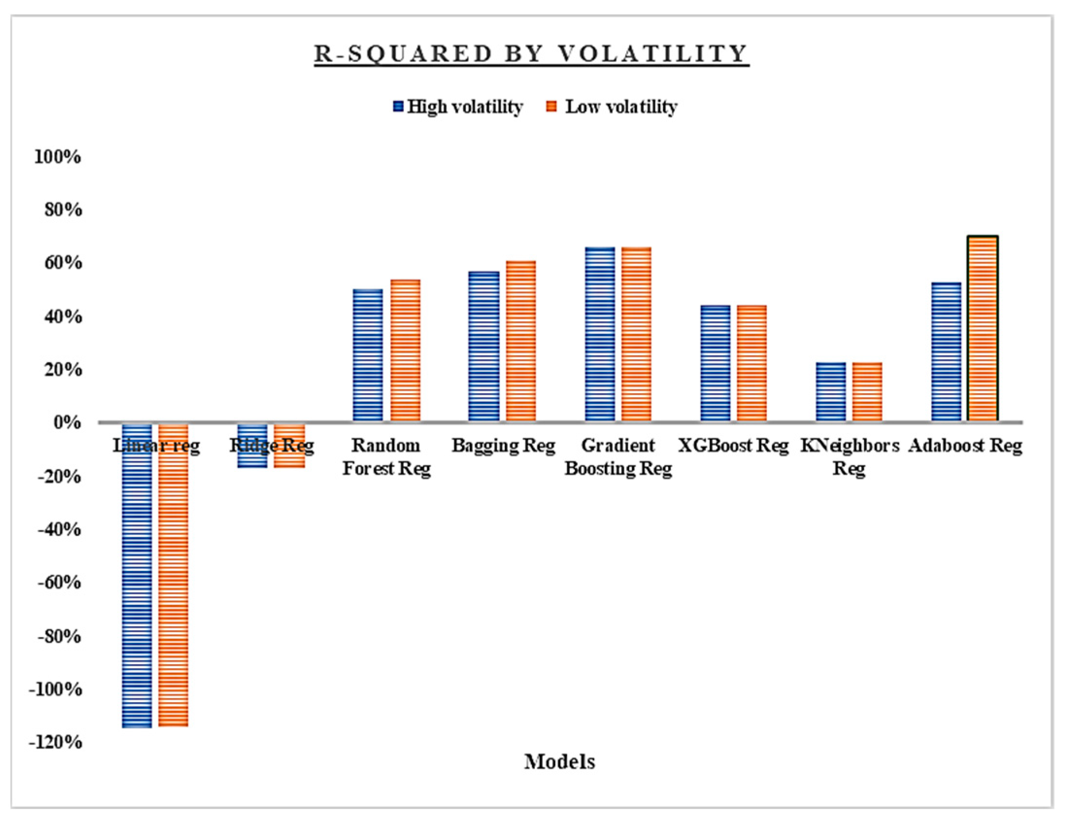
Appendix C.1. Grouping by Volatility by Targets: High Volatility
| Models | Residuals | Mean Squared Error | R-Squared | Mean Cross Validation Score |
| Linear regression | −59,327,819.08 | 3.103195 × 10²⁰ | −1.144 | −253.80 |
| Ridge Regression | −40,263,611.43 | 1.699994 × 10²⁰ | −0.17 | −29.18 |
| Random Forest Regressor | −28,879,206.47 | 7,216,968 × 108 | 0.50 | −0.85 |
| Bagging Regressor | −28,411,174.11 | 6,158,571 × 108 | 0.57 | −3.34 |
| Gradient Boosting Regressor | −17,772,056.50 | 4,940,930 × 108 | 0.66 | −1.55 |
| XGBoost Regressor | −28,289,899.56 | 7,986,635 × 108 | 0.44 | −0.94 |
| KNeighbors Regressor | −29,801,474.76 | 1.1108049 × 10²⁰ | 0.23 | −0.32 |
| Adaboost Regressor | −7,268,139.56 | 64,677,311 × 108 | 0.53 | −0.60 |
Appendix C.2. Grouping by Volatility by Targets: Low Volatility
| Models | Residuals | Mean Squared Error | R-Squared | Mean Cross Validation Score |
| Linear regression | −59,327,819.08 | 3.103195 × 10²⁰ | −1.14 | −253.80 |
| Ridge Regression | −40,263,611.43 | 1.699994 × 10²⁰ | −0.17 | −29.18 |
| Random Forest Regressor | −28,455,959.39 | 6,675,874 × 107 | 0.54 | −0.89 |
| Bagging Regressor | −297,537 × 102 | 244,154 × 109 | 0.61 | −1.35 |
| Gradient Boosting Regressor | −17,282,934.1 | 491,648 × 108 | 0.66 | −1.99 |
| XGBoost Regressor | −28,289,899.56 | 7,986,635 × 108 | 0.44 | −0.94 |
| KNeighbors Regressor | −34,832,710.33 | 1.1108049 × 10²⁰ | 0.23 | −0.32 |
| Adaboost Regressor | −7,268,139.56 | 4,388,766 × 108 | 0.70 | −0.97 |
Appendix D. Year-on-Year Change in CO2 Emissions for the Considered Countries

References
- Patel, S.S.; McCaul, B.; Cáceres, G.; Peters, L.E.R.; Patel, R.B.; Clark-Ginsberg, A. Delivering the promise of the Sendai Framework for Disaster Risk Reduction in fragile and conflict-affected contexts (FCAC): A case study of the NGO GOAL’s response to the Syria conflict. Prog. Disaster Sci. 2021, 10, 100172. [Google Scholar] [CrossRef]
- Garschagen, M.; Doshi, D.; Reith, J.; Hagenlocher, M. Global patterns of disaster and climate risk—An analysis of the consistency of leading index-based assessments and their results. Clim. Chang. 2021, 169, 11. [Google Scholar] [CrossRef]
- Kim, B.J.; Jeong, S.; Chung, J.-B. Research trends in vulnerability studies from 2000 to 2019: Findings from a bibliometric analysis. Int. J. Disaster Risk Reduct. 2021, 56, 102141. [Google Scholar] [CrossRef]
- Shi, P.; Ye, T.; Wang, Y.; Zhou, T.; Xu, W.; Du, J.; Wang, J.; Li, N.; Huang, C.; Liu, L.; et al. Disaster Risk Science: A Geographical Perspective and a Research Framework. Int. J. Disaster Risk Sci. 2020, 11, 426–440. [Google Scholar] [CrossRef]
- Bloice, L.; Burnett, S. Barriers to knowledge sharing in third sector social care: A case study. J. Knowl. Manag. 2016, 20, 125–145. [Google Scholar] [CrossRef]
- Mukendi, C.M.; Choi, H. Temporal Analysis of World Disaster Risk: A Machine Learning Approach to Cluster Dynamics. In Proceedings of the 2023 14th International Conference on Information and Communication Technology Convergence (ICTC), IEEE, Jeju Island, Republic of Korea, 11–13 October 2023; pp. 973–978. [Google Scholar] [CrossRef]
- IHME, Global Burden of Disease Study. Deaths That Are from All Causes Attributed to Air Pollution per 100,000 People, in Both Sexes Aged Age-Standardized. 2019. Available online: https://ourworldindata.org/air-pollution (accessed on 15 December 2023).
- Li, S.; Siu, Y.W.; Zhao, G. Driving Factors of CO2 Emissions: Further Study Based on Machine Learning. Front. Environ. Sci. 2021, 9, 721517. [Google Scholar] [CrossRef]
- Venditti, B. Here’s How CO2 Emissions Have Changed since 1900. In Proceedings of the World Economic Forum, El Sheikh, Egypt, 22 November 2022; Available online: https://www.weforum.org/agenda/2022/11/visualizing-changes-carbon-dioxide-emissions-since-1900/ (accessed on 15 December 2023).
- James, G.; Witten, D.; Hastie, T.; Tibshirani, R.; Taylor, J. Linear Regression. In An Introduction to Statistical Learning; Springer Texts in Statistics; Springer International Publishing: Cham, Switzerland, 2023; pp. 69–134. [Google Scholar] [CrossRef]
- Özkale, M.R.; Altuner, H. Bootstrap confidence interval of ridge regression in linear regression model: A comparative study via a simulation study. Commun. Stat. Theory Methods 2023, 52, 7405–7441. [Google Scholar] [CrossRef]
- Pérez-Rodríguez, J.; Fernández-Navarro, F.; Ashley, T. Estimating ensemble weights for bagging regressors based on the mean–variance portfolio framework. Expert Syst. Appl. 2023, 229, 120462. [Google Scholar] [CrossRef]
- Ghunimat, D.; Alzoubi, A.E.; Alzboon, A.; Hanandeh, S. Prediction of concrete compressive strength with GGBFS and fly ash using multilayer perceptron algorithm, random forest regression and k-nearest neighbor regression. Asian J. Civ. Eng. 2023, 24, 169–177. [Google Scholar] [CrossRef]
- Cai, J.; Xu, K.; Zhu, Y.; Hu, F.; Li, L. Prediction and analysis of net ecosystem carbon exchange based on gradient boosting regression and random forest. Appl. Energy 2020, 262, 114566. [Google Scholar] [CrossRef]
- Zhao, W.P.; Li, J.; Zhao, J.; Zhao, D.; Lu, J.; Wang, X. XGB Model: Research on Evaporation Duct Height Prediction Based on XGBoost Algorithm. Radioengineering 2020, 29, 81–93. [Google Scholar] [CrossRef]
- Wei, H. AdaBoost Regression Predicts the Ranking of College Students Using the Super Star Learning APP. In Proceedings of the 2023 IEEE International Conference on Electrical, Automation and Computer Engineering (ICEACE), Changchun, China, 29–31 December 2023; pp. 355–362. [Google Scholar] [CrossRef]
- Yao, B. Walmart Sales Prediction Based on Decision Tree, Random Forest, and K Neighbors Regressor. Highlights Bus. Econ. Manag. 2023, 5, 330–335. [Google Scholar] [CrossRef]
- Boateng, E.Y.; Abaye, D.A. A Review of the Logistic Regression Model with Emphasis on Medical Research. J. Data Anal. Inf. Process. 2019, 7, 190–207. [Google Scholar] [CrossRef]
- Charbuty, B.; Abdulazeez, A. Classification Based on Decision Tree Algorithm for Machine Learning. J. Appl. Sci. Technol. Trends 2021, 2, 20–28. [Google Scholar] [CrossRef]
- Shaik, A.B.; Srinivasan, S. A Brief Survey on Random Forest Ensembles in Classification Model. In International Conference on Innovative Computing and Communications; Bhattacharyya, S., Hassanien, A.E., Gupta, D., Khanna, A., Pan, I., Eds.; Lecture Notes in Networks and Systems; Springer: Singapore, 2019; Volume 56, pp. 253–260. ISBN 9789811323539. [Google Scholar] [CrossRef]
- Abdurrahman, G.; Sintawati, M. Implementation of xgboost for classification of parkinson’s disease. J. Phys. Conf. Ser. 2020, 1538, 012024. [Google Scholar] [CrossRef]
- Chandramouli, A.; Hyma, V.R.; Tanmayi, P.S.; Santoshi, T.G.; Priyanka, B. Diabetes prediction using Hybrid Bagging Classifier. Entertain. Comput. 2023, 47, 100593. [Google Scholar] [CrossRef]
- Hao, L.; Huang, G. An improved AdaBoost algorithm for identification of lung cancer based on electronic nose. Heliyon 2023, 9, e13633. [Google Scholar] [CrossRef] [PubMed]
- Gezici, B.; Tarhan, A.K. Explainable AI for Software Defect Prediction with Gradient Boosting Classifier. In Proceedings of the 2022 7th International Conference on Computer Science and Engineering (UBMK), Diyarbakir, Turkey, 14–16 September 2022; pp. 1–6. [Google Scholar] [CrossRef]
- Alam, S.; Sonbhadra, S.K.; Agarwal, S.; Nagabhushan, P. One-class support vector classifiers: A survey. Knowl. Based Syst. 2020, 196, 105754. [Google Scholar] [CrossRef]
- Naiem, S.; Khedr, A.E.; Idrees, A.M.; Marie, M.I. Enhancing the Efficiency of Gaussian Naïve Bayes Machine Learning Classifier in the Detection of DDOS in Cloud Computing. IEEE Access 2023, 11, 124597–124608. [Google Scholar] [CrossRef]
- Raschka, S. Model Evaluation, Model Selection, and Algorithm Selection in Machine Learning. arXiv 2018, arXiv:1811.12808. [Google Scholar] [CrossRef]
- Hodson, T.O.; Over, T.M.; Foks, S.S. Mean Squared Error, Deconstructed. J. Adv. Model. Earth Syst. 2021, 13, e2021MS002681. [Google Scholar] [CrossRef]
- Ma, Y.; Xie, Z.; Chen, S.; Qiao, F.; Li, Z. Real-time detection of abnormal driving behavior based on long short-term memory network and regression residuals. Transp. Res. Part C Emerg. Technol. 2023, 146, 103983. [Google Scholar] [CrossRef]
- Chicco, D.; Warrens, M.J.; Jurman, G. The coefficient of determination R-squared is more informative than SMAPE, MAE, MAPE, MSE and RMSE in regression analysis evaluation. PeerJ Comput. Sci. 2021, 7, e623. [Google Scholar] [CrossRef] [PubMed]
- Heydarian, M.; Doyle, T.E.; Samavi, R. MLCM: Multi-Label Confusion Matrix. IEEE Access 2022, 10, 19083–19095. [Google Scholar] [CrossRef]
- Kharwal, A.M.N. Classification Report in Machine Learning. Available online: https://www.mendeley.com/catalogue/bb23c245-6fe2-37d1-a8ba-4041334de8c9/ (accessed on 15 December 2023).
- Chicco, D.; Jurman, G. The advantages of the Matthews correlation coefficient (MCC) over F1 score and accuracy in binary classification evaluation. BMC Genom. 2020, 21, 6. [Google Scholar] [CrossRef] [PubMed]
- Christoph, M. Interpretable Machine Learning: PArtial Dependence Plot. Available online: https://christophm.github.io/interpretable-ml-book/pdp.html (accessed on 15 December 2023).
- Molnar, C.; Freiesleben, T.; König, G.; Herbinger, J.; Reisinger, T.; Casalicchio, G.; Wright, M.N.; Bischl, B. Relating the Partial Dependence Plot and Permutation Feature Importance to the Data Generating Process. In Explainable Artificial Intelligence; Longo, L., Ed.; Communications in Computer and Information Science; Springer Nature: Cham, Switzerland, 2023; Volume 1901, pp. 456–479. ISBN 978-3-031-44063-2. [Google Scholar] [CrossRef]
- Kong, G.; Hu, S.; Yang, Q. Uncertainty method and sensitivity analysis for assessment of energy consumption of underground metro station. Sustain. Cities Soc. 2023, 92, 104504. [Google Scholar] [CrossRef]
- Iooss, B.; Saltelli, A. Introduction to Sensitivity Analysis. In Handbook of Uncertainty Quantification; Ghanem, R., Higdon, D., Owhadi, H., Eds.; Springer International Publishing: Cham, Switzerland, 2015; pp. 1–20. ISBN 978-3-319-11259-6. [Google Scholar] [CrossRef]
- Akour, I.; Rahamneh, A.A.; Al Kurdi, B.; Alhamad, A.; Al-Makhariz, I.; Alshurideh, M.; Al-Hawary, S. Using the Canonical Correlation Analysis Method to Study Students’ Levels in Face-to-Face and Online Education in Jordan. Inf. Sci. Lett. 2023, 12, 901–910. [Google Scholar] [CrossRef]
- Yin, Y.; Jang-Jaccard, J.; Xu, W.; Singh, A.; Zhu, J.; Sabrina, F.; Kwak, J. IGRF-RFE: A hybrid feature selection method for MLP-based network intrusion detection on UNSW-NB15 dataset. J. Big Data 2023, 10, 15. [Google Scholar] [CrossRef]
- Zhai, J.; Kong, F. The Impact of Multi-Dimensional Urbanization on CO2 Emissions: Empirical Evidence from Jiangsu, China, at the County Level. Sustainability 2024, 16, 3005. [Google Scholar] [CrossRef]
- Ngcobo, R.; De Wet, M.C. The Impact of Financial Development and Economic Growth on Renewable Energy Supply in South Africa. Sustainability 2024, 16, 2533. [Google Scholar] [CrossRef]
- Global Carbon Budget. Year-On-Year Change in CO₂ Emissions—GCB. 2023. Available online: https://ourworldindata.org/grapher/absolute-change-co2 (accessed on 15 December 2023).
- Jones; Matthew, W.; Peters, G.P.; Gasser, T.; Andrew, R.M.; Schwingshackl, C.; Gütschow, J.; Houghton, R.A.; Friedlingstein, P.; Pongratz, J.; et al. Annual Greenhouse Gas Emissions by World Region [Dataset]. National Contributions to Climate Change [Original Data]. 2023. Available online: https://ourworldindata.org/grapher/ghg-emissions-by-world-region (accessed on 16 December 2023).
- Wei, T.; Wu, J.; Chen, S. Keeping Track of Greenhouse Gas Emission Reduction Progress and Targets in 167 Cities Worldwide. Front. Sustain. Cities 2021, 3, 696381. [Google Scholar] [CrossRef]
- Copernicus Climate Change Service. ‘Annual Temperature Anomalies’ [Dataset]. Copernicus Climate Change Service, ‘ERA5 Monthly Averaged Data on Single Levels from 1940 to Present 2’ [Original Data]. 2024. Available online: https://ourworldindata.org/grapher/annual-temperature-anomalies (accessed on 15 December 2023).
- NASA’s Scientific Visualization Studio. Global Temperature Anomalies from 1880 to 2019. Scientific Visualization Studio. Available online: https://svs.gsfc.nasa.gov/4787#section_credits (accessed on 15 December 2023).
- Global Carbon Budget. ‘Other Industry—GCB’ [Dataset]. Global Carbon Project, ‘Global Carbon Budget’ [Original Data]. 2023. Available online: https://ourworldindata.org/grapher/co2-by-source (accessed on 15 December 2023).
- Molteni, M.; Walker, G.; Parmar, D.; Sutton, M.; Licence, P.; Woodward, S. Can “Electric Flare Stacks” Reduce CO2 Emissions? A Case Study with Nonthermal Plasma. Ind. Eng. Chem. Res. 2023, 62, 19649–19657. [Google Scholar] [CrossRef]
- Concrete needs to lose its colossal carbon footprint. Nature 2021, 597, 593–594. [CrossRef] [PubMed]
- Global Carbon Budget. ‘Cumulative CO2 emissions—GCB’ [Dataset]. Global Carbon Project, ‘Global Carbon Budget’ [Original data]. 2023. Available online: https://ourworldindata.org/grapher/cumulative-co-emissions (accessed on 15 December 2023).
- Liu, Z.; Deng, Z.; Davis, S.J.; Giron, C.; Ciais, P. Monitoring global carbon emissions in 2021. Nat. Rev. Earth Environ. 2022, 3, 217–219. [Google Scholar] [CrossRef] [PubMed]
- Global Carbon Budget. ‘Share of Global Cumulative CO2 Emissions—GCB’ [Dataset]. Global Carbon Project, ‘Global Carbon Budget’ [Original Data]. 2023. Available online: https://ourworldindata.org/grapher/share-of-cumulative-co2 (accessed on 15 December 2023).
- Gillett, N.P. Warming proportional to cumulative carbon emissions not explained by heat and carbon sharing mixing processes. Nat. Commun. 2023, 14, 6466. [Google Scholar] [CrossRef]
- Jones; Matthew, W.; Peters, G.P.; Gasser, T.; Andrew, R.M.; Schwingshackl, C.; Gütschow, J.; Houghton, R.A.; Friedlingstein, P.; Pongratz, J.; et al. ‘Contribution to Global Mean Surface Temperature Rise’ [Dataset]. ‘National Contributions to Climate Change’ [Original Data]. 2023. Available online: https://ourworldindata.org/grapher/contribution-temp-rise-degrees (accessed on 15 December 2023).
- Ritchie, H.; Rosado, P.; Roser, M. Data Page: Global Warming: Contributions to the Change in Global Mean Surface Temperature. Available online: https://ourworldindata.org/grapher/contributions-global-temp-change (accessed on 15 December 2023).
- World Population Prospects. ‘Growth Rate—Sex: All—Age: All—Variant: Estimates’ [Dataset]. UN. 2023. Available online: https://ourworldindata.org/grapher/population-growth-rates (accessed on 15 December 2023).
- The Connections Between Population and Climate Change Info Brief. Washington, 2024. Available online: https://populationconnection.org/resources/population-and-climate/ (accessed on 15 December 2023).
- Gapminder—Population v7 (2022), Gapminder—Systema Globalis (2022), HYDE (2017), and United Nations—World Population Prospects (2022), ‘Population (Future Projections) (Future Projections)’ [dataset]. Gapminder, ‘Population v7’; Gapminder, ‘Systema Globalis’; PBL Netherlands Environmental Assessment Agency, ‘HYDE 3.2’; United Nations, ‘World Population Prospects’ [original data]. 2023. Available online: https://ourworldindata.org/grapher/population-long-run-with-projections (accessed on 15 December 2023).
- Centre, W. No Education. [Dataset]. Wittgenstein Centre (2018) [Original Data]. 2023. Available online: https://ourworldindata.org/grapher/world-population-level-education (accessed on 15 December 2023).
- Tang, M.M.; Xu, D.; Lan, Q. How does education affect urban carbon emission efficiency under the strategy of scientific and technological innovation? Front. Environ. Sci. 2023, 11, 1137570. [Google Scholar] [CrossRef]
- Word Bank. GDP (Constant 2015 US$). 2023. Available online: https://data.worldbank.org/indicator/NY.GDP.MKTP.KD (accessed on 15 December 2023).
- Word Bank. GDP per Capita (Constant 2015 US$). 2023. Available online: https://data.worldbank.org/indicator/NY.GDP.PCAP.KD (accessed on 15 December 2023).
- Vigna, L.; Friedrich, J. Global per Capita Emissions Explained—Through 9 Charts. Available online: https://www.weforum.org/agenda/2023/05/global-per-capita-emissions-explained-charts/ (accessed on 15 December 2023).
- World Bank; OECD. ‘GDP’ [Dataset]. 2023. Available online: https://ourworldindata.org/grapher/co2-gdp-growth (accessed on 15 December 2023).


| Category Names | Min Values | Max Values | Range | Countries |
|---|---|---|---|---|
| High positive | 3.244667 × 10³ | 6.769703 × 10⁸ | 676,967,055.333 | United States, China, India |
| High negative | −1.906534 × 10⁸ | −1.370680 × 10⁵ | 190,516,332 | |
| Moderate positive | 4.88107 × 10⁵ | 3.741389 × 10⁷ | 36,925,079.3 | United Kingdom, France, South Korea, Brazil, India |
| Moderate negative | −3.209079 × 10⁷ | −4.587947 × 10⁵ | 31,631,995.3 | |
| Low positive | 2.683000 × 10³ | 2.632321 × 10⁷ | 26,320,527 | South Africa, Nigeria, Democratic Republic of the Congo |
| Low negative | −2.045842 × 10⁷ | −8.609333 × 10³ | 20,449,810.667 |
| Model | MCC | AUC | Precision | Recall | F1 Score | Mean CV |
|---|---|---|---|---|---|---|
| Logreg | 0.67 | 0.73 | 0.76 | 0.73 | 0.68 | 0.74 |
| DT | 0.95 | 0.96 | 0.96 | 0.96 | 0.96 | 0.93 |
| RF | 0.87 | 0.89 | 0.91 | 0.89 | 0.89 | 0.86 |
| XGB | 0.83 | 0.85 | 0.89 | 0.85 | 0.84 | 0.91 |
| GB | 0.84 | 0.86 | 0.89 | 0.86 | 0.85 | 0.85 |
| SVC | 0.58 | 0.64 | 0.70 | 0.64 | 0.58 | 0.73 |
| MLP | 0.60 | 0.66 | 0.74 | 0.66 | 0.64 | 0.75 |
| GNB | 0.50 | 0.58 | 0.66 | 0.58 | 0.55 | 0.75 |
| Confusion Matrix | Precision | Recall | F1-Score | Support | ||||||
| High negative | 12 | 0 | 0 | 0 | 0 | 0 | 0.71 | 1.00 | 0.83 | 12 |
| High positive | 0 | 27 | 0 | 0 | 0 | 0 | 1.00 | 1.00 | 1.00 | 27 |
| Low negative | 0 | 0 | 15 | 0 | 1 | 0 | 1.00 | 0.94 | 0.97 | 16 |
| Low positive | 0 | 0 | 0 | 23 | 0 | 0 | 0.96 | 1.00 | 0.98 | 23 |
| Moderate negative | 5 | 0 | 0 | 0 | 28 | 0 | 0.97 | 0.85 | 0.90 | 33 |
| Moderate positive | 0 | 0 | 0 | 1 | 0 | 18 | 1.00 | 0.95 | 0.97 | 19 |
| High negative | High positive | Low negative | Low positive | Moderate negative | Moderate positive | |||||
| Class | Increase | Decrease |
|---|---|---|
| High negative |
| 3-year average |
| High positive |
| --- |
| Low negative | --- |
|
| Low positive |
|
|
| Moderate negative |
|
|
| Moderate positive |
|
|
| Features | High Negative | High Positive | Moderate Negative | Moderate Positive | Low Negative | Low Positive |
|---|---|---|---|---|---|---|
| Population (number) | 4.81 × 10⁸ | 8.07 × 10⁸ | 7.18 × 10⁷ | 7.91 × 10⁷ | 6.74 × 10⁷ | 6.74 × 10⁷ |
| CO2 from coal | 1.45 × 10⁹ | 1.76 × 10⁹ | 1.15 × 10⁸ | 1.24 × 10⁸ | 1.04 × 10⁸ | 8.21 × 10⁷ |
| Mean-3y | −7.31 × 10⁷ | 1.07 × 10⁸ | −1.07 × 10⁷ | 1.06 × 10⁷ | −3.02 × 10⁶ | 4.76 × 10⁶ |
| GDP | 9.99 × 10¹² | 4.27 × 10¹² | 1.96 × 10¹² | 9.79 × 10¹¹ | 1.72 × 10¹¹ | 1.38 × 10¹¹ |
| CO2 from oil | 1.58 × 10⁹ | 8.85 × 10⁸ | 2.12 × 10⁸ | 1.71 × 10⁸ | 2.43 × 10⁷ | 2.31 × 10⁷ |
| Population—Education: Incomplete Primary | 2.04 × 10⁷ | 4.32 × 10⁷ | 2.10 × 10⁶ | 5.82 × 10⁶ | 3.90 × 10⁶ | 3.94 × 10⁶ |
| Contribution to temperature rise | 0.173045 | 0.098758 | 0.029083 | 0.022507 | 0.010212 | 0.008529 |
Disclaimer/Publisher’s Note: The statements, opinions and data contained in all publications are solely those of the individual author(s) and contributor(s) and not of MDPI and/or the editor(s). MDPI and/or the editor(s) disclaim responsibility for any injury to people or property resulting from any ideas, methods, instructions or products referred to in the content. |
© 2024 by the authors. Licensee MDPI, Basel, Switzerland. This article is an open access article distributed under the terms and conditions of the Creative Commons Attribution (CC BY) license (https://creativecommons.org/licenses/by/4.0/).
Share and Cite
Mukendi, C.M.; Choi, H.; Jung, S.; Kim, Y.-S. Determinants of Yearly CO2 Emission Fluctuations: A Machine Learning Perspective to Unveil Dynamics. Sustainability 2024, 16, 4242. https://doi.org/10.3390/su16104242
Mukendi CM, Choi H, Jung S, Kim Y-S. Determinants of Yearly CO2 Emission Fluctuations: A Machine Learning Perspective to Unveil Dynamics. Sustainability. 2024; 16(10):4242. https://doi.org/10.3390/su16104242
Chicago/Turabian StyleMukendi, Christian Mulomba, Hyebong Choi, Suhui Jung, and Yun-Seon Kim. 2024. "Determinants of Yearly CO2 Emission Fluctuations: A Machine Learning Perspective to Unveil Dynamics" Sustainability 16, no. 10: 4242. https://doi.org/10.3390/su16104242
APA StyleMukendi, C. M., Choi, H., Jung, S., & Kim, Y.-S. (2024). Determinants of Yearly CO2 Emission Fluctuations: A Machine Learning Perspective to Unveil Dynamics. Sustainability, 16(10), 4242. https://doi.org/10.3390/su16104242