Analysis of the Driving Mechanism of Urban Carbon Emission Correlation Network in Shandong Province Based on TERGM

Abstract

Analyzing the driving factors and mechanisms of urban carbon emission correlation networks can provide effective carbon reduction decision-making support for Shandong Province and other regions with similar industrial characteristics. Based on industrial carbon emission data from various cities in Shandong Province from 2013 to 2021, the spatial correlation network of carbon emission was established by using a modified gravity model. The characteristics of the network were explored by using the Social Network Analysis (SNA) method, and significant factors affecting the network were identified through Quadratic Assignment Procedure (QAP) correlation analysis and motif analysis. The driving mechanism of the carbon emission correlation network was analyzed by using Temporal Exponential Random Graph Models (TERGMs). The results show that: (1) The spatial correlation network of urban carbon emission in Shandong Province exhibits multi-threaded complex network correlations with a relatively stable structure, overcoming geographical distance limitations. (2) Qingdao, Jinan, and Rizhao have high degree centrality, betweenness centrality, and closeness centrality in the network, with Qingdao and Jinan being relatively central. (3) Shandong Province can be spatially clustered into four regions, each with distinct roles, displaying a certain “neighboring clustering” phenomenon. (4) Endogenous network structures such as Mutual, Ctriple, and Gwesp significantly impact the formation and evolution of the network, while Twopath does not show the expected impact; FDI can promote the generation of carbon emission reception relationships in the spatial correlation network; IR can promote the generation of carbon emission spillover relationships in the spatial correlation network; GS, differences in GDP, differences in EI, and similarities of IR can promote the generation of organic correlations within the network; on the temporal level, the spatial correlation network of urban carbon emission in Shandong Province has shown significant stability during the study period.

1. Introduction

In order to promote regional development, China actively implements major regional coordinated development strategies such as the coordinated development of the Beijing Tianjin Hebei region, the development of the Yangtze River Economic Belt, ecological protection in the Yellow River Basin, and high-quality development. Regional integration policies, convenient industrial connections, natural geographical proximity, and spatial spillovers of carbon emissions themselves may all promote local agglomeration of carbon emissions, thereby forming a carbon emission correlation network based on economic production and consumption activities across the country, composed of nodes or small groups of different scales. As the province with the third GDP and the second population in China, Shandong Province has made remarkable achievements in green and low-carbon development since speeding up the replacement of old growth drivers with new ones in 2017. However, according to the data of carbon emission accounts and datasets (CEADs), Shandong has consistently ranked first among all provinces in China in terms of carbon emissions, indicating that it still needs to strengthen carbon emission reduction. In 2022, the People’s Government of Shandong Province issued the “Peak Implementation Plan for Carbon Peak in Shandong Province”, proposing that by 2025, carbon dioxide emissions per unit of regional GDP will be reduced by 20.5% compared with 2020, and by 2030, carbon dioxide emissions per unit of regional GDP will be reduced by more than 68% compared with 2005, so as to ensure that the target of carbon peak before 2030 will be achieved on schedule. The realization of Shandong’s carbon reduction target requires the joint efforts of 16 municipalities under its jurisdiction. Differences in city size, resource allocation, industrial structure, technological progress, and other aspects lead to uneven distribution of carbon emissions among cities. In the process of pursuing rapid economic growth, Shandong Province actively promotes the regional development framework of “one group, two centers, and three circles”. However, this initiative inadvertently promotes the concentration of local carbon emissions while promoting inter-city cooperation within the region. The interconnectivity of adjacent cities in industrial activities, product exchange, transportation, and other aspects, as well as the spillover effect of carbon emissions themselves, further catalyzes the formation of a network of carbon emissions among cities. Accurately characterizing the spatial correlation network of urban carbon emission and elucidating its driving force and mechanism are of great significance for understanding the spatial evolution of carbon emission in Shandong Province. This understanding will facilitate the development of precise and comprehensive regional collaborative emission reduction strategies and, to a certain extent, provide relevant research ideas and strategic references for other urban agglomerations, provinces, and even the whole country.

When analyzing the spatial correlation of carbon emission, scholars used various methods, including global spatial autocorrelation Moran’s I index, local spatial autocorrelation Moran’s I index, and aggregation map, to conduct exploratory spatial data analysis (ESDA) in different research areas, and then concluded that regional carbon emissions exhibit significant spatial correlation [1,2,3,4,5]. Considering the intricate nonlinear network relationships inherent in regional carbon emissions, scholars used Social Network Analysis (SNA) to construct spatial correlation networks, analyzing overall network characteristics [6,7] and individual network characteristics [8,9]. In addition, scholars used the iterative correlation convergence method (CONCOR) for spatial clustering analysis [10,11].

To delve deeper into the driving mechanism of the spatial correlation network of carbon emission, scholars conducted correlation or regression analyses by using the Quadratic Assignment Procedure (QAP) on the basis of SNA [12,13,14]. In addition to the geographical spatial proximity [15], the factors considered in these analyses also include the differences in the economic development level [16], energy consumption [17], industrial structure [18], environmental policy [19], urbanization rate [20], and foreign direct investment [21].

However, the Quadratic Assignment Procedure (QAP) usually only considers the impact of individual attribute variables on the network, occasionally involving external environment variables. The Exponential Random Graph Model (ERGM) addresses a limitation of QAP analysis by considering the impact of individual attribute variables on the network and incorporating the influence of endogenous network structure [22], external environment [23], and other factors. In recent years, ERGM has been applied in environmental studies. For instance, Gong et al. utilized the ERGM method to investigate the evolution mechanism of the spatial network of natural gas consumption [24]. Similarly, Dong et al. employed ERGM to examine the factors influencing the formation of the spatial correlation network of carbon emission efficiency [25]. While ERGM has been increasingly applied in environmental studies, particularly in exploring network dynamics, it is primarily used for analyzing static networks. This limitation restricts its effectiveness in analyzing the evolving nature of networks over time and may hinder its ability to capture time dependence and causality within the network [26].

In the realm of complex network research, scholars have advanced their studies to explore multi-period networks by using the Temporal Exponential Random Graph Model (TERGM) on the basis of ERGM [27]. By considering the correlation of network data across different time points, TERGM effectively addresses the time-dependent nature of longitudinal observation network data, surpasses the constraints of static network analysis methods, and enhances the analysis of dynamic changes in network structures [28]. In recent years, TERGM has found widespread application in various fields, such as trade networks [29,30,31,32,33], technical cooperation [34], and land transfers [35]. While Cai et al. were the first to propose TERGM for urban carbon emissions, their model only considers urban GDP as an individual attribute variable [36], indicating limitations in variable selection.

Although scholars have conducted extensive research on the characteristics and driving mechanism of the spatial correlation network of carbon emissions, the current research still has the following shortcomings: Firstly, in terms of methodology, the factors covered by TERGM are more comprehensive and objective, but the selection of individual attribute effects and exogenous network effect variables within TERGM is often determined through qualitative descriptions provided by scholars, rather than through exploratory quantitative analysis. Secondly, as for the research object, there is no relevant research on the spatial correlation network of urban carbon emission in a province by using TERGM.

Given this, we select 16 cities within Shandong Province as the focal research subjects. Initially, we employ Quadratic Assignment Procedure (QAP) correlation analysis to identify the principal factors influencing the formation of the correlation network. Subsequently, motif analysis is utilized to derive the endogenous network structure variables. These steps facilitate the construction of a Temporal Exponential Random Graph Model (TERGM) for the urban carbon emissions correlation network in Shandong Province. Through this model, we meticulously analyze the driving mechanisms behind the evolution of the spatial correlation network, aiming to furnish actionable recommendations for enhancing carbon emission reduction efforts in Shandong Province. The innovation contribution of this paper mainly has two aspects: (1) The main driving factors leading to the formation of the correlation network are obtained by using QAP analysis, which provides the basis for the selection of individual attribute effect and exogenous network effect variables in TERGM. (2) The spatial correlation network of urban carbon emission in Shandong Province is constructed to clarify the driving mechanism of the evolution of the correlation network by using TERGM analysis, which provides the basis for formulating specific policy recommendations.

The paper is structured into the following sections: Section 2 provides data sources and research techniques. Section 3 analyzes the individual and overall characteristics of the spatial correlation network of urban carbon emission in Shandong Province and screens for endogenous network structure variables, individual attribute variables, and network covariates. Section 4 delves into the research results obtained from analyzing the driving mechanism of carbon emission spatial correlation networks. The Section 5 summarizes the main research findings, proposes policy recommendations, and summarizes the limitations of this study and some directions for future research.

2. Methodology and Data

2.1. Social Network Analysis

2.1.1. The Modified Gravity Model

Drawing on the practices of scholars [37], we constructed a modified gravity model based on factors such as the Gross Domestic Product (GDP) of Shandong Province, carbon emissions, population, and geographical distance. This model aims to analyze the degree of carbon emission correlation among cities under the influence of economic and social connections. The modified model is as follows:

$$C_{ij}=k_{ij}\frac{\sqrt[3]{P_i{G}_i{E}_i}\sqrt[3]{P_j{G}_j{E}_j}}{d_{ij}^2},\hspace{1em}\hspace{1em}{k}_{ij}=\frac{E_i}{E_i+E_j}$$

(1)

where i and j represent different cities; C_ij represents the carbon emission correlation value between city i and city j; P_i, G_i, and E_i, respectively, represent the total population of city i at the end of the year, GDP of city i, and CO₂ emissions of city i; k_ij is the gravitational coefficient between the two cities, and d_ij is the distance between the two cities.

The gravity matrix can be obtained from Formula (1), with the row mean of the matrix as the threshold. If the gravity value is greater than this threshold, it is marked as 1, indicating the existence of a correlation. If the gravity value is less than the threshold, it is marked as 0, indicating no correlation. This analysis identifies urban carbon emission spatial correlation relationships with strong gravitational, forms the spatial correlation matrix, and constructs the spatial correlation network of carbon emission on this basis.

2.1.2. Overall Network Analysis

Drawing on the practices of scholars [38], we selected four indicators: number of network correlations, network density, network hierarchy, and network efficiency to depict the overall characteristics of the correlation network. The number of network correlations reflects the number of edges within the correlation network, revealing the interconnections among nodes. Network density measures the closeness of contact among nodes; the higher the value, the tighter the connections among cities in terms of carbon emissions. Network efficiency measures the efficiency of connections among nodes; the higher the value, the fewer the network connections, indicating the complexity and stability of the network are lower. Network hierarchy indicates the status of each node within the network; networks of the lower hierarchy have lower asymmetric accessibility among nodes, meaning there are fewer unidirectional correlations in the network, and the status of each node is relatively balanced.

2.1.3. Individual Network Analysis

Drawing on the practices of scholars [39], we used three indicators: degree centrality, betweenness centrality, and closeness centrality to analyze the individual characteristics of the correlation network. Degree centrality reflects the extent to which a node occupies a central position; the higher the value, the greater the number of direct connections between the city represented by the point and other cities, meaning the city is closer to the center of the network, and its influence on the network is more significant. Closeness centrality describes the ability of a node to be independent of the influence of other nodes, meaning nodes with higher closeness centrality represent cities that are less likely to be controlled by other cities in the network. Betweenness centrality shows the ability of a node to control correlations among other nodes; the higher the value, the stronger the ability of a node to control carbon emission correlations among other nodes in the network, indicating that the city represented by the node plays a greater “mediator” role in the network.

2.1.4. Block Model Analysis

Simplifying complex networks into “block models” can clearly demonstrate the overall pattern of the network. Following the method of Wasserman et al. [40], we divided the spatial correlation network of urban carbon emission in Shandong Province into four blocks through spatial clustering analysis. The net beneficiary block receives a relatively higher number of relationships both within and outside the block, with the number of received relationships significantly exceeding the number of emitted relationships. The net outflow block has a higher number of emitted relationships than received relationships. The bidirectional outflow block has a relatively balanced number of received and emitted relationships, and there are more relationships within the block. The broker block has a relatively balanced number of received and emitted relationships, but there are fewer relationships within the block.

2.1.5. QAP Correlation Analysis

Quadratic Assignment Procedure (QAP) correlation analysis is often used to evaluate the correlation among multiple relational matrices. Drawing on the research achievements of scholars [15,16,17,18,19,20,21], we initially selected factors such as economic development level, urbanization rate, industrial structure, digitization level, energy intensity, investment level, external openness level, environmental regulation, and geographical spatial proximity as variables. The definition of each variable is given in

Table 1. Variable definitions in the QAP correlation analysis.

Variable Type	Variable Name	Variable Symbols
Economic Development Level	Gross Domestic Product	GDP
	Per Capita GDP	NGDP
Industrial Structure	Industrialization Rate	IR
	Proportion of Tertiary Industry GDP	TI
Energy Intensity	Energy Consumption Intensity	EI
Urbanization Rate	Urbanization Rate	UR
Digitization Level	Digital Inclusive Finance Index [41]	DE
Investment Level	The Amount of Fixed Asset Investment	IFA
External Openness Level	Proportion of Actually Utilized Foreign Direct Investment in GDP	FDI
Environmental Regulation	Proportion of Environmental Governance Investment in GDP	IEG
Geographical Spatial Proximity	Reciprocal Matrix of Geographical Distance	GS

.

The above variables (except for GS) were processed into corresponding difference matrices. Through QAP correlation analysis, we explored the correlation between the carbon emissions correlation matrix over the years and each indicator matrix, and the factors that passed the significance test were screened out. These factors serve as individual attribute variables and exogenous network variables for subsequent Temporal Exponential Random Graph Models (TERGMs) analysis.

2.2. Motif Structure Analysis

Motifs, which are locally small connected subgraphs, play a significant role in the formation of networks. Ma et al. pointed out that the p-value measures the probability that the frequency of a motif structure in the random network is higher than that in the real network; at the same time, the Z-value represents the ratio of the difference between the number of occurrences of a motif structure in the real network and that in the random network to the standard deviation of the number of occurrences of the motif structure in the random network [42]. Therefore, a smaller p-value means that the motif structure is more common in the real network, and a p-value of 1 indicates that the motif structure is invalid; a higher Z-value indicates that the motif structure is more important in the real network, and a non-positive Z-value indicates that the motif structure is invalid. Based on this, by counting the distribution frequency of various typical motifs in different periods and conducting p-value and Z-value analyses, we identified vital motif structures to provide a basis for selecting structural variables for subsequent Temporal Exponential Random Graph Models (TERGMs) analysis.

2.3. Temporal Exponential Random Graph Model

The Temporal Exponential Random Graph Model (TERGM) is a statistical model used for analyzing and simulating the temporal evolution of network data. It is based on the theoretical framework of the Exponential Random Graph Model (ERGM) and captures the dynamic changes of network structure with time by introducing time dimension. TERGM can provide a probabilistic description of edge changes within the network, facilitating the analysis of time dependency in the formation and dissolution of network connections. Compared to ERGM, TERGM integrates the element of time, enabling the formulation of the following model:

$$P\left(Y=y^t\left|y^{t-k},\dots y^{t-1},\theta \right.\right)=\frac{exp\left({\sum }_l{\theta }_l^{T}f(y^t, y^{t-1},\dots y^t)\right)}{c(\theta ,\left|y^{t-k}, \right.\dots y^{t-1})}$$

(2)

The above equation represents the probability of the explained variable $y^t$ occurring in the network set $Y$ under condition $\theta$; $c(\theta ,\left|y^{t-k}, \right.\dots y^{t-1})$ is a normalization constant to ensure that the probabilities derived from the model are within the range of [0, 1]; l represents the related structural effects and attributes that influence the formation of network relations; $f(y^t, y^{t-1},\dots y^t)$ is a proxy variable for l, including endogenous structural variables, individual attribute variables, and exogenous network covariates; ${\theta }_l$ refers to the estimated parameters corresponding to each variable, which are used to determine the influence degree of different factors on the evolution of the carbon emission correlation network based on their significance, positivity or negativity, and magnitude. Where $y^t$ represents the correlation network at time t, and $y^{t-k}$ to $y^{t-1}$ represent the correlation networks from lag k to lag 1 periods.

However, Model (2) only yields the probability for the t-th period formed by a k-order Markov chain based on discrete time. Therefore, we obtained the probability distribution of the network time series by calculating the joint probability between time k + 1 and T as follows:

$$P\left(y^{k+1},\dots ,y^T\left|y^1,\dots y^k,\theta \right.\right)={\prod }_{t=k+1}^{T}P\left(Y=y^t\left|y^{t-k},\dots y^{t-1},\theta \right.\right)$$

(3)

We employed the btergm package in R to compute TERGM, used the Markov Chain Monte Carlo Maximum Likelihood Estimation (MCMC MLE) method for simulation and parameter adjustment of the constructed model, and resulted in stable model parameters.

2.4. Data Source and Processing

We selected the data from 16 cities in Shandong Province from 2013 to 2021 as the research sample. Apart from geographical distance and carbon emission data, other data are sourced from the “China City Statistical Yearbook”, “Shandong Statistical Yearbook”, and statistical yearbooks of various prefecture-level cities. To ensure the comparability of the data, monetary unit variables such as GDP and Per Capita GDP were deflated to constant 2012 prices.

The carbon emission data were calculated based on the carbon emission conversion method provided by the Intergovernmental Panel on Climate Change (IPCC). Energy consumption data are sourced from the “Shandong Provincial Statistical Yearbook” and statistical yearbooks of various prefecture-level cities over the years; the geographical distance data chosen are the ArcGIS distances among cities.

3. Characteristics of Spatial Correlation Network of Carbon Emission

3.1. Overall Network Structural Characteristics

A carbon emission gravity matrix for Shandong Province was constructed by using the modified gravity model, while network diagrams for 2013, 2016, 2019, and 2021 were created by using Gephi 0.10.1, as shown in Figure 1. During the period from 2013 to 2021, the spatial correlation network of carbon emissions in Shandong Province changed little, showing a trend of stable development form and complexity. At the same time, there are no isolated points in the network for each period, indicating that there is a certain carbon emission correlation among cities within the province.

Through the analysis of correlation networks from 2013 to 2021, we obtained the values of four indicators: number of network correlations, network density, network efficiency, and network hierarchy, as shown in

Table 2. Overall characteristic index values of the spatial correlation network of carbon emission in Shandong Province from 2013 to 2021.

Year	Number of Network Correlations	Network Density	Network Efficiency	Network Hierarchy
2013	53	0.221	0.7905	0.125
2014	53	0.221	0.7905	0.125
2015	52	0.217	0.8	0.125
2016	51	0.213	0.8095	0.125
2017	51	0.213	0.8095	0.125
2018	52	0.217	0.8	0.125
2019	51	0.213	0.81	0.125
2020	51	0.213	0.8095	0.125
2021	51	0.213	0.8095	0.125
Average	52	0.2157	0.8032	0.125

. The number of network correlations fluctuated between 51 and 53, and the network density varied between 0.213 and 0.221, both displaying a “decline-rise-decline-stable” trend with minor numerical changes, indicating that the spatial correlation network structure of carbon emissions in Shandong Province was relatively stable. The average number of network connections was 52, which was significantly lower than the potential maximum number of network connections (240), resulting in a low network density of only 0.2157 on average; it suggested that the tightness of the spatial correlation network of carbon emission in Shandong Province was not high, indicating there was considerable room for collaborative improvement. The network efficiency increased from 0.7905 in 2013 to 0.8095 in 2021, with an average network efficiency of 0.8032; on the one hand, it indicated that the complexity and stability of the spatial correlation network structure of carbon emissions in Shandong Province had slightly decreased, meaning there was still much room to strengthen the correlations among cities; on the other hand, it suggested that there was still a certain proportion of redundant connections in the network, meaning there were multiple overlapping overflow channels. The network hierarchy remained stable at 0.125 throughout the study period, indicating that the spatial correlation network structure of carbon emission was stable; the low network hierarchy suggested fewer unidirectional associations among cities within the network, indicating that the status of cities was relatively balanced.

3.2. Individual Network Structural Characteristics

The status and role of each city within the spatial correlation network of carbon emission can be characterized by indicators such as degree centrality, betweenness centrality, and closeness centrality. Limited to the length of the article, we selected the results for 2021 as an example to analyze, as shown in

Table 3. Analysis results of carbon emission network centrality in Shandong Province in 2021.

City	Degree Centrality				Betweenness Centrality		Closeness Centrality
	Centrality	Out-Degree	In-Degree	Sorting	Centrality	Sorting	Centrality	Sorting
Jinan	53.33	5	11	2	69.00	2	75.00	2
Qingdao	63.33	5	14	1	84.33	1	93.75	1
Zibo	10.00	2	1	13	1.57	9	53.57	12
Zaozhuang	20.00	4	2	5	26.50	4	57.69	4
Dongying	13.33	4	0	10	0.00	14	57.69	5
Yantai	20.00	3	3	6	3.50	7	57.69	6
Weifang	16.67	2	3	8	0.67	13	55.56	10
Jining	20.00	4	2	7	15.00	6	57.69	7
Taian	10.00	2	1	14	1.57	10	53.57	13
Weihai	13.33	2	2	11	0.00	15	51.72	16
Rizhao	26.67	4	4	3	24.00	5	60.00	3
Linyi	23.33	4	3	4	41.50	3	57.69	8
Dezhou	10.00	2	1	15	1.57	11	53.57	14
Liaocheng	10.00	2	1	16	1.57	12	53.57	15
Binzhou	16.67	3	2	9	3.23	8	57.69	9
Heze	13.33	3	1	12	0.00	16	55.56	11
Average	21.25	3.19	3.19		17.13		59.50

.

In terms of degree centrality, Qingdao (QD), Jinan (JN), Rizhao (RZ), and Linyi (LY) ranked in the top four, and their values were above average, indicating that these cities had a more significant influence on the network and were closer to the center of the network. However, QD and JN exhibited a significantly higher degree centrality compared to other cities, suggesting that QD and JN occupy the core leading position in the network. In addition, the in-degree values of cities such as JN, QD, and Yantai (YT) were higher than their out-degree values, indicating that these cities mainly played the role of receivers in the network; it showed that these cities had higher “prestige” to attract carbon emission spillovers in other cities. Furthermore, the out-degree values of cities such as Zaozhuang (ZZ), Jining (JNN), Binzhou (BZ), Dongying (DY), Heze (HZ), Zibo (ZB), Taian (TA), Dezhou (DZ), and Liaocheng (LC) were higher than their in-degree values, indicating that these cities primarily acted as senders within the network. Particularly, the out-degree value of DY significantly exceeded its in-degree value, and this phenomenon may be related to its abundant resources such as oil and natural gas; the unique natural advantage of DY also provides solid energy support for the economic development of other cities in Shandong Province.

Regarding betweenness centrality, QD, JN, LY, ZZ, and RZ ranked in the top five, and their values were above average, indicating that these cities played the role of “intermediaries” within the spatial correlation network of carbon emission and possessed greater control for the connections of the network, especially JN and QD, which were relatively central. However, other cities had relatively low betweenness centrality values, which were below average, suggesting that their control for the connections of the network was weak. Particularly, DY, Weihai (WH), and HZ had a betweenness centrality of zero, indicating they were almost in the controlled position within the network.

In terms of closeness centrality, QD, JN, and RZ ranked in the top three, and their values were above average; it showed that these cities had a strong ability to break away from control within the spatial correlation network of carbon emission, meaning that they can more efficiently establish carbon emission connections with other cities and were less likely to be controlled by others. In particular, the closeness centrality values of QD and JN were significantly higher than the values of other cities, which further confirmed their core leading position and great influence in the spatial correlation network of carbon emission. Further analysis of the closeness centrality values of most other cities showed that the gap was small, which further confirmed the relative balance of cities in the spatial correlation network of carbon emission; however, their values were lower than average, indicating that their ability to break away from the control of other cities in the spatial correlation network of carbon emission was relatively weak.

3.3. Block Model Analysis

We employed the CONCOR algorithm to categorize the cities within the spatial correlation network of carbon emission in Shandong Province into four major blocks: net beneficiaries, net spillovers, bidirectional spillovers, and brokers. The results are as shown in

Table 4. Correlations among carbon emission network space blocks in Shandong Province in 2021.

Block	Number of Cities	Sending Relationships		Receiving Relationships		Expected Internal Relationship Ratio (%)	Actual Internal Relationship Ratio (%)	Block Properties
		Internal Block	External Block	Internal Block	External Block
Block One	4	7	9	7	9	20	43.75	Bidirectional spillovers
Block Two	6	1	14	1	5	33.33	6.67	Net spillovers
Block Three	3	6	4	6	13	13.33	60	Net beneficiaries
Block Four	3	4	6	4	6	13.33	40	Brokers

: Block one included JN, JNN, ZZ, and HZ, where the number of sending and receiving relations was balanced; compared to other blocks, block one exhibited more spatial correlations internally, so it was the bidirectional spillover block. Block two included ZB, DY, BZ, LC, TA, and DZ, where the number of sending relations exceeded the receiving ones significantly, indicating they had a strong carbon spillover tendency, so block two was classified as the net spillover block. Block three contained QD, WH, and YT; the number of receiving relationships inside and outside the block was relatively large, and the number of receiving relationships was greater than the number of sending relationships, so block three was the net beneficiary block. Block four included RZ, Weifang (WF), and LY; the number of sending and receiving relations of this block was relatively balanced, and the connections within the block were relatively few; combined with the analysis of Table 3, it was evident that cities like RZ and LY played the intermediary role of “bridge” in the overall network, so block four was the broker block.

To obtain a more intuitive observation of the positions of each block, the cities they encompass, and the relationships among these cities, we utilized ArcGIS 10.8 to create Figure 2 and Figure 3. The geographical location of Shandong Province in China and the spatial distribution of cities in Shandong Province are shown in Figure 2. Figure 3 reveals that cities within the same block tended to gather, indicating that carbon emission spillovers were related to geographical factors. The adjacent areas influenced the carbon emissions of each city to some extent, which also laid the foundation for introducing geographical proximity variables in the subsequent sections.

3.4. Network Motif Structure Analysis

To gain a deeper understanding of the microstructure of the spatial correlation network of carbon emission in Shandong Province and to provide the basis for selecting structural variables for subsequent Temporal Exponential Random Graph Model (TERGM) analysis, we utilized Mavisto V2.7.0 to statistically analyze the motif structures of the spatial correlation network of carbon emission in Shandong Province from 2013 to 2021. Due to limited length, we focused on the triad motif statistical results of the 2021 carbon emission correlation network and the key triad motif structures for the years 2013, 2016, 2019, and 2021, as shown in

Table 5. Triad motif structures of the spatial correlation network of carbon emission in Shandong Province in 2021.

Code	Triad Motif	Frequency	p-Value	Z-Value	Code	Triad Motif	Frequency	p-Value	Z-Value
F8X		86	0	4.536	JQF		14	0.829	−0.567
GCX		145	0	2.757	FKX		43	0.999	−3.462
GDF		31	0	3.838	F8R		173	1	−5.759
FMF		17	0	3.060	GOX		8	1	−4.239
GQX		20	0.02	2.955	GCR		165	1	0.000
K4F		3	0.031	2.123	F7F		65	1	0.000
IMF		22	0.68	−0.336

and

Table 6. Key triad motif structures of the spatial correlation network of carbon emission in Shandong Province in 2013, 2016, 2019, and 2021.

Sorting	2013			2016			2019			2021
	Code	Frequency	Z-Value	Code	Frequency	Z-Value	Code	Frequency	Z-Value	Code	Frequency	Z-Value
1	GCX	148	2.690	GCX	145	2.707	GCX	145	2.762	GCX	145	2.757
2	F8X	88	4.174	F8X	86	4.655	F8X	86	4.519	F8X	86	4.536
3	GDF	31	3.626	GDF	31	3.781	GDF	31	3.838	GDF	31	3.838
4	GQX	21	2.811	GQX	20	3.039	GQX	20	2.810	GQX	20	2.955
5	FMF	18	3.040	FMF	17	3.279	FMF	17	3.128	FMF	17	3.060

.

As can be seen from Table 5, the p-values of motif structures such as F7F, GCR, GOX, and F8R were 1, and their Z-values were non-positive, indicating they are invalid in the network. Similarly, motifs such as IMF, JQF, and FKX had larger p-values and non-positive Z-values, suggesting that these complex motif structures were also invalid in the network. Conversely, the p-values of the motifs such as F8X, GCX, GDF, and FMF were 0, and their Z-values were positive; additionally, the p-values of the motifs such as GQX and K4F were less than 0.05, and their Z-values were positive, indicating that these six motifs significantly impacted the formation of the spatial correlation network of carbon emission and that reciprocal connection patterns were likely to be relatively stable. Among the motifs with a p-value of 0, GCX, F8X, and GDF were the most frequently occurring structures. Their characteristic was that one node connected to two other nodes through bidirectional or unidirectional relationships, while the other two nodes did not connect, indicating that many cities within the spatial correlation network of carbon emission in Shandong Province formed connections through an intermediary third city, thereby highlighting the role of cities in the broker block.

Table 6 shows that in 2013, 2016, 2019, and 2021, the key triad motifs with p-values of 0 or close to 0 (less than 0.05) and positive Z-values, ranked from highest to lowest frequency, are consistently GCX, F8X, GDF, GQX, and FMF, indicating that structures characterized by reciprocity, connectivity, cyclicity, and clustering play a significant role in the formation of relationships within the spatial correlation network of carbon emission. These findings provided a basis for selecting structural variables in subsequent TERGM analysis.

3.5. QAP Correlation Analysis

The spatial correlation matrices of carbon emission over the years, difference matrices for various indicators, and the geographical proximity matrix were analyzed by conducting a Quadratic Assignment Procedure (QAP). The results for 2021 are given in

Table 7. QAP correlation analysis of the spatial correlation network and influencing factors of carbon emission in 2021.

Variable	Correlation Coefficient	Significance Level	Variable	Correlation Coefficient	Significance Level
GDP	0.536 ***	0.000	EI	0.049 **	0.012
NGDP	0.084	0.238	IFA	−0.501	0.199
UR	0.112	0.135	FDI	0.287 *	0.055
IR	−0.121 **	0.023	IEG	0.117	0.187
TI	0.394	0.251	GS	0.397 ***	0.000
DE	0.010	0.411

Note: ***, **, and * indicate significance at the 1%, 5%, and 10% levels, respectively.

.

Among the indicators tested, GDP and GS passed the significance test at the 1% level; IR and EI passed the significance test at the 5% level; FDI passed the significance test at the 10% level.

4. Analysis of Network Driving Mechanism Based on TERGM

4.1. Variable Selection

The driving factors of the Temporal Exponential Random Graph Model (TERGM) include endogenous network structural variables, individual attribute variables, network covariates, and time-dependency items.

Table 8. TERGM statistics of the formation mechanism of the spatial correlation network of urban carbon emission.

Variable Type	Variable	Schematic Diagram
Endogenous Network Structural Variable	Edges
	Mutual
	Twopath
	Ctriple
	Gwesp
Individual Attribute Variable	Nodeocov
	Nodeicov
	Absdiff
Network Covariate	Edgecov
Time-Dependency Item	Stability
	Variability

shows the pattern of variables.

4.1.1. Endogenous Network Structural Variables

Based on the results of motif structure analysis, we found that the spatial correlation network of urban carbon emission in Shandong Province exhibited the micro-association pattern characterized by reciprocity (Mutual), connectivity (Twopath), cyclicity (Ctriple), and clustering (Gwesp). Therefore, we selected Edges, Mutual, Twopath, Ctriple, and Gwesp as structural variables for the TERGM analysis.

4.1.2. Individual Attribute Variables and Network Covariates

Through the QAP correlation analysis of the initially selected relevant indicators, the main driving factors leading to the formation of the spatial correlation network of carbon emission were identified, namely GDP, IR, EI, FDI, and GS. We selected GDP, IR, EI, and FDI as individual attribute variables, and their impact on the network was manifested as sender effect (Sender), receiver effect (Receiver), and heterophily (Absdiff); GS was selected as the network covariate.

4.1.3. Time-Dependency Items

In terms of time variables, we selected stability and variability as indicators. Stability was used to represent the temporal stability of the network and to measure whether the connection state of the spatial correlation network is stable from period t − 1 to t. Variability was used to represent the dynamic development of the network and to detect whether the connection state changes or disappears across periods, which was helpful in exploring whether the formation and evolution of the network might interact with time in a suppressive manner.

4.2. Analysis of TERGM Regression Results

As shown in

Table 9. Results of the TERGM.

Variable Type	Variable Name	Model 1	Model 2	Model 3
Endogenous Network Structural Variable	Edges	−5.75 *** (0.78)	−2.73 *** (0.53)	−1.79 *** (0.41)
	Mutual		7.55 *** (0.72)	2.58 *** (0.59)
	Twopath		0.07 (0.09)	0.04 (0.19)
	Ctriple		−2.98 *** (0.42)	−1.08 *** (0.28)
	Gwesp		1.10 *** (0.18)	0.69 ** (0.29)
Time-Dependency Item	Stability			6.40 *** (1.24)
	Variability			0.16 (0.22)
Individual Attribute Variable	Receiver (GDP)	−0.05 (0.45)	−0.10 (0.55)	−2.19 (3.37)
	Sender (GDP)	0.05 (0.47)	0.37 (0.60)	2.46 (3.51)
	Absdiff (GDP)	6.26 *** (0.49)	6.12 *** (0.60)	3.99 *** (0.78)
	Receiver (FDI)	1.39 *** (0.17)	1.85 *** (0.23)	3.18 ** (1.38)
	Sender (FDI)	−0.45 ** (0.16)	−1.03 *** (0.22)	−0.93 ** (0.38)
	Absdiff (FDI)	0.79 (1.46)	1.92 (1.64)	0.84 (1.51)
	Receiver (EI)	−2.97 *** (0.64)	−3.84 *** (0.79)	−5.84 *** (0.42)
	Sender (EI)	0.19 (0.56)	0.16 (0.67)	3.13 (3.75)
	Absdiff (EI)	0.78 * (0.36)	1.93 *** (0.55)	1.42 *** (0.25)
	Receiver (IR)	−6.72 (4.09)	−3.89 (4.98)	−2.37 (4.14)
	Sender (IR)	5.30 ** (2.21)	2.71 *** (0.37)	1.34 ** (0.53)
	Absdiff (IR)	−1.49 *** (0.32)	−1.14 *** (0.38)	−1.03 *** (0.33)
Network Covariate	Edgecov (GS)	6.84 *** (0.48)	7.65 *** (0.66)	9.77 ** (3.98)
Fit Index	AIC	768.43	640.54	577.71
	BIC	864.96	815.06	744.55

Note: ***, **, and * indicate significance at the 1%, 5%, and 10% levels, respectively.

, the regression results were obtained by inputting the spatial correlation matrices of carbon emission from 2013 to 2021, cross-sectional data of related variables, and the reciprocal matrix of geographical distance into the Temporal Exponential Random Graph Model (TERGM). Model 1 was the benchmark model that included individual attribute variables and network covariates. Model 2 was the integrated model that incorporated endogenous network structural variables, and Model 3 was the comprehensive model with time-dependency items. By progressively adding variables and continuously adjusting the models, it was observed that from Model 1 to Model 3, the values of the model fit indicators Akaike Information Criterion (AIC) and Bayesian Information Criterion (BIC) gradually decreased, indicating that the internal and external structures of the model were continuously improving, and the fit of the model was getting better and better, which can adequately explain the driving mechanism of the spatial correlation network of urban carbon emission in Shandong Province.

4.2.1. Impact of Endogenous Network Structure

As indicated in Table 9, both Mutual and Ctriple passed the significance test at the 1% level, and Gwesp also passed the significance test at the 5% level; however, Twopath did not reach the 10% significance level, showing that Mutual, Ctriple, and Gwesp significantly impacted the formation of the network, while Twopath did not reach the expected level of impact. Furthermore, the results from Model 2 and Model 3 showed that the significance levels of the structural variables did not vary significantly, and the sign of the coefficients remained unchanged, indicating that the results of the structural variables were relatively robust. Therefore, the following analysis primarily focused on the comprehensive Model 3, which analyzed the driving mechanism of the spatial correlation network of urban carbon emission in Shandong Province.

(1) Mutual: The impact coefficient of Mutual was significantly positive, indicating that the active interaction among cities within the spatial correlation network of carbon emission in Shandong Province can promote the formation of bidirectional connections of carbon emission; Yuan et al. obtained similar results when studying the spatial correlation network of traffic carbon emissions in China [43]; it meant that the cooperation among cities in carbon emission reduction was more effective for overall carbon emission reduction.

(2) Twopath: The influence coefficient of Twopath was not significant; on the one hand, it showed that the cities in the spatial correlation network of carbon emission might exhibit a high degree of independence in their emission behaviors, meaning that the change in carbon emissions in one city might not directly affect other cities, or the effect was not enough to be reflected in the overall structure of the network; on the other hand, it showed that the indirect relationships (such as the connection through intermediary nodes) played an important role in the spatial correlation network of carbon emission, which meant that the impact of carbon emissions might spread through a long path or multiple intermediary nodes, rather than through direct one-to-one connections.

(3) Ctriple: The impact coefficient of Ctriple was significantly negative; on the one hand, it showed that in the spatial correlation network of carbon emission, structures of triangular cycle transmission were less, which meant that the market mechanism alone was not enough to achieve the optimal transfer of carbon emissions, but needed complementary advantages and collaborative regulation between the market mechanism and government regulation; on the other hand, it showed that the spatial transmission of carbon emissions has a certain direction, for example, from cities with the relatively developed economy to cities with the relatively backward economy, or from cities with relatively abundant energy to cities with less abundant energy, which may be related to the structure of the urban industrial chain in Shandong Province; for example, some cities served as the supply bases of raw materials or energy, while others were the centers of processing, manufacturing, or consumption.

(4) Gwesp: The impact coefficient of Gwesp was significantly positive, showing that there were highly clustered sub-networks in the spatial correlation network of carbon emission, and cities were closely connected in terms of carbon emission correlations; it might be due to their economic activities, energy use, and other related factors.

4.2.2. Impact of Individual Attributes

(1) GDP: The receiver effect and sender effect coefficients of GDP were −2.19 and 2.46, respectively, but neither of them passed the significance test, indicating that the driving effect of GDP on the receiving effect and sending effect in the spatial correlation network of carbon emission was not obvious. However, the absdiff of the GDP was significantly positive, which indicated that the greater the difference in GDP among cities, the more likely it was to form correlations of carbon emissions; when Wei et al. investigated the spatial correlation and influencing factors of carbon emission intensity within the Guangdong–Hong Kong–Macao Great Bay Area (GBA), they highlighted that the increase in regional differences in the level of economic development would often lead to a closer spatial correlation network of carbon emission intensity [44]; this phenomenon might be related to the pattern of economic complementarity and regional cooperation between cities with high GDP and cities with low GDP in Shandong Province; for example, accelerating the development planning of the integration of Jinan-Zibo, Jinan-Taian, and Jinan-Dezhou had led to the organic correlation of carbon emissions among cities with large differences in GDP.

(2) FDI: The receiver effect coefficient of FDI was significantly positive, while the sender effect coefficient was significantly negative, which meant that within the spatial correlation network of urban carbon emission in Shandong Province, cities with high levels of openness (such as QD, YT, and WH) tended to become receivers of carbon emission activities in other cities and were less likely to “export” carbon directly to other cities; it aligned with the conclusion from the block model analysis that these cities played a net beneficiary role, and the reason might be that cities with the higher levels of openness usually have stronger economic strength and better infrastructure, which can attract foreign investment and the transfer of high-carbon industries. However, the absdiff of FDI did not pass the significance test, which showed that the difference in openness level among cities had no significant impact on the formation of carbon emission correlation. Similarly, both Wang et al. and Liu et al. found that the difference matrix of FDI failed the significance test, and the conclusion that the increase in FDI can improve environmental pollution is still unclear [45,46].

(3) EI: The receiver effect coefficient of EI was significantly negative, meaning that within the spatial correlation network of urban carbon emission in Shandong Province, cities with higher energy consumption intensity (such as BZ and ZB) were less likely to be receivers of carbon emission activities in other cities, and these cities also belonged to the net spillover block; it verified the previous analysis of “less receiving” in cities of this block. The sender effect coefficient was positive but not significant, indicating that cities with high energy consumption intensity tended to “export” carbon to other cities in the spatial correlation network of urban carbon emission, but it was not obvious. The absdiff coefficient of EI was significantly positive, indicating that within the spatial correlation network of urban carbon emission in Shandong Province, cities with high energy consumption intensity and cities with low energy consumption intensity were more likely to form heterophily connections. In the previous study of Guan et al., it was found that the difference in energy intensity can indeed promote the formation of spatial correlation of industrial carbon emissions, which is consistent with the results of this paper [47]; it may be because they were complementary in energy use and management to improve energy efficiency and reduce carbon emissions.

(4) IR: The receiver effect coefficient of IR was negative but not significant, indicating that the tendency of cities with a high industrialization rate to become receivers of carbon emission activities in other cities was not significant. The sender effect coefficient of IR was significantly positive, meaning that cities with a high industrialization rate tended to “export” carbon to other cities in the spatial correlation network of carbon emission; it reflected that some cities in Shandong Province still impacted the carbon emissions of other cities through the industry chain and energy supply chain in the process of low-carbon transformation. The significantly negative absdiff coefficient of IR meant that cities with similar industrialization rates were more likely to form correlations of carbon emissions; similarly, Wang et al. emphasized that the difference in industrial structure would reduce the spatial spillover of carbon emissions to a certain extent, resulting in the reduction of correlation [48]; it might be related to the agglomeration of related industries when Shandong province promoted the construction of a new regional development pattern of “one group, two centers, and three circles”; this series of regional cooperation aimed to share low-carbon technologies, optimize energy structure, and promote industrial upgrading to achieve the common goal of reducing carbon emissions.

4.2.3. Impact of External Environmental

The coefficient of GS is significantly positive, indicating that it can promote the formation and evolution of the spatial correlation network of urban carbon emission in Shandong Province. Liao et al. emphasized that geographical distance is negatively correlated with the formation of the spatial correlation network of carbon emissions, which means that the closer the geographical distance, the more convenient the transportation of many resources and industrial transfer, and the shorter the distance is conducive to the formation of the spatial correlation network of carbon emissions. The GS in this paper refers to the reciprocal matrix of geographical distance, and the results are consistent [49]. Geographically close cities tended to form carbon emission correlations; specifically, coastal cities in Shandong Province, such as QD, YT, and WH, were not only geographically adjacent but also closely linked in terms of economic development and port logistics, which might lead to stronger correlations in carbon emissions among them; similarly, inland cities within the province, such as JN and ZB, might also exhibit stronger correlations in the carbon emission correlation network due to more frequent industrial cooperation and energy flows facilitated by geographical proximity, which further proved that overall reduction actions of carbon emission need to be jointly implemented through regional cooperation and coordinated actions.

4.2.4. Impact of Time-Dependency Items

(1) Stability: The coefficient of stability was significantly positive, indicating that the spatial correlation network of carbon emission in Shandong Province had significant stability over time; it was also confirmed by the morphological stability of the spatial correlation network of carbon emission at different time points.

(2) Variability: The coefficient of variability was significantly positive; on the one hand, it meant that the spatial correlation network of carbon emission in Shandong Province has little change in time, and the network structure did not change randomly or frequently; on the other hand, it indicated that in the network, the carbon emission correlation patterns among cities were relatively stable, and there would not be large-scale reorganizations or changes in the short term.

4.3. Robustness Test

To verify the robustness of the research results, referring to the sample period segmentation method proposed by Dong et al. [50], the years 2013–2021 were divided into three periods: 2013–2015, 2016–2018, and 2019–2021, and TERGM regression was carried out for each period, respectively. The specific results, as shown in

Table 10. TERGM robustness test results.

Variable Type	Variable Name	2013–2015	2016–2018	2019–2021
Endogenous Network Structural Variable	Edges	−1.16 *** (0.17)	−3.75 *** (0.69)	−1.31 *** (0.24)
	Mutual	5.36 *** (1.00)	6.65 *** (1.30)	6.05 *** (1.25)
	Twopath	0.22 (0.18)	0.15 (0.21)	0.18 (0.26)
	Ctriple	−2.85 *** (0.67)	−2.10 *** (0.64)	−2.63 *** (0.76)
	Gwesp	1.40 *** (0.33)	1.18 *** (0.32)	1.23 *** (0.38)
Time-Dependency Item	Stability	5.34 *** (1.26)	3.62 *** (1.08)	5.79 *** (1.47)
	Variability	0.33 (0.78)	0.72 (0.89)	0.02 (0.11)
Individual Attribute Variable	Receiver (GDP)	−0.38 (3.27)	−0.65 (0.71)	−0.40 (1.06)
	Sender (GDP)	0.40 (3.43)	0.74 (0.95)	0.58 (1.15)
	Absdiff (GDP)	0.87 *** (0.23)	1.25 *** (0.16)	0.97 *** (0.32)
	Receiver (FDI)	1.60 ** (0.63)	1.87 ** (0.78)	1.69 * (0.81)
	Sender (FDI)	−0.71 ** (0.29)	−1.55 *** (0.42)	−1.72 ** (0.65)
	Absdiff (FDI)	0.27 (0.49)	1.95 (3.11)	−1.37 (5.48)
	Receiver (EI)	−1.44 *** (0.25)	−1.45 ** (0.61)	−2.16 ** (0.88)
	Sender (EI)	2.33 (4.11)	1.58 (1.81)	−2.00 (2.46)
	Absdiff (EI)	1.39 *** (0.44)	1.79 *** (0.47)	1.06 ** (0.43)
	Receiver (IR)	−2.52 (4.27)	−2.37 (1.84)	−2.26 (3.47)
	Sender (IR)	1.18 ** (0.51)	1.87 * (0.85)	1.93 ** (0.74)
	Absdiff (IR)	−4.28 *** (1.15)	−5.90 ** (2.36)	−3.87 ** (1.52)
Network Covariate	Edgecov (GS)	6.42 *** (0.93)	6.97 *** (1.08)	6.74 *** (1.16)

Note: ***, **, and * indicate significance at the 1%, 5%, and 10% levels, respectively.

, indicated that the influence direction and significance of each variable in the model estimates for different periods were basically consistent with those of Model 3, meaning that the results of Model 3 were robust.

4.4. Goodness-of-Fit Test

To verify the rationality and scientific nature of the results of Model 3, we selected typical statistical indicators such as Degree, Edge-wise shared partners, Dyad-wise shared partners, Geodesic distances, Triad census, and the Receiver Operating Characteristic (ROC) curve for the goodness-of-fit test. The results are shown in Figure 4. Leifeld et al. pointed out that when the black solid line falls near the dotted line in the middle of the box, it means that the measurement results of the actual observation network overlap with the 95% confidence interval of the simulated network measurements, indicating that the model fits well [51]. Pan et al. pointed out that the closer the ROC curve is to the upper left corner and the closer the PR curve is to the upper right corner, the better the model fit [52]. When checking the fitting diagram of the model, it was obvious that in the first five subgraphs, most of the black solid lines were closely aligned with the dotted line in the center of the box; in the sixth subgraph, the ROC curve (red) and the PR curve (blue) tended to the upper left corner and upper right corner, respectively. This alignment showed that the model fitted well, indicating that the TERGM model successfully simulated the structural characteristics of the observation network. Consequently, Model 3 can provide valuable, scientific, and reasonable insights into the mechanism of network evolution.

5. Conclusions and Policy Implications

Based on the relevant data from various cities in Shandong Province from 2013 to 2021, we constructed the spatial correlation network of urban carbon emission in Shandong Province by using the modified gravity model; we analyzed the structural characteristics of the network by conducting Social Network Analysis (SNA) and Motif Structure Analysis; we selected individual attribute variables by utilizing Quadratic Assignment Procedure (QAP); finally, the Temporal Exponential Random Graph Model (TERGM) was used to analyze the driving mechanism of the formation and evolution of the network. The main conclusions are as follows:

(1) From the perspective of the overall network structure, the spatial correlation network of carbon emission in Shandong Province breaks the limitations of geographical spatial distance, displaying multi-threaded complex network correlations, and the network structure remains relatively stable. The network density was small and stable, indicating there was significant room for enhancing the spatial correlation of carbon emission in Shandong Province; the network efficiency was high and relatively stable, suggesting that the complexity of the network was low, with some space for improvement; the network hierarchy was low and stable, indicating nodes within the spatial correlation network of urban carbon emission were a relatively balanced status, and the network structure is relatively stable.

(2) From the perspective of individual network structure, in terms of degree centrality, QD, JN, RZ, and LY had higher values, indicating that they had a greater impact on the spatial correlation network of carbon emission. JN, QD, and YT had in-degrees that were higher than out-degrees, playing the role of receivers; ZZ, JNN, BZ, DY, and HZ had out-degrees that were higher than in-degrees, playing the role of senders. In terms of betweenness centrality, QD, JN, LY, ZZ, and RZ had higher values, indicating their “mediator” role was significant in the spatial correlation network of carbon emission; however, other cities had weaker control over the spatial correlation network, especially DY, WH, and HZ. In terms of closeness centrality, QD, JN, and RZ had higher values, indicating their ability to evade control was strong in the spatial correlation network of carbon emission; however, other cities had smaller values and gaps, which showed their ability to evade control from other cities was relatively weaker in the spatial correlation network, indicating that cities were in the relatively balanced state within the spatial correlation network.

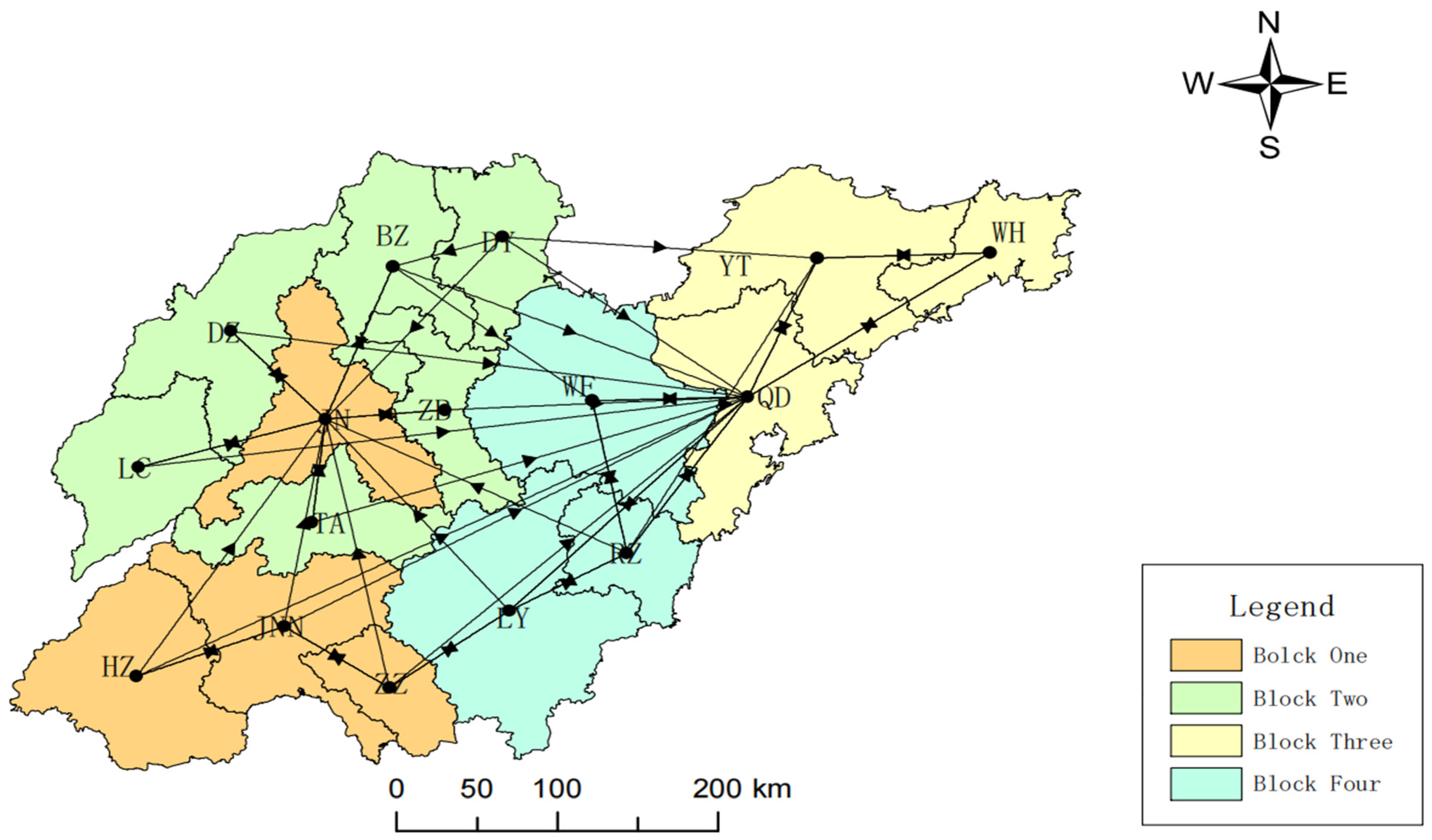
(3) From the perspective of spatial clustering, Shandong Province can be divided into four blocks: JN, JNN, ZZ, and HZ formed Block One, playing a role of “bidirectional spillover”; ZB, DY, BZ, LC, TA, and DZ formed Block Two, playing a role of “net spillover”; QD, WH, and YT formed Block Three, playing a role of “net beneficiary”; and RZ, WF, and LY formed Block Four, playing a role of “broker”.

(4) From the perspective of driving mechanism analysis, significant structural variables such as Mutual, Twopath, Ctriple, and Gwesp in the network were screened out through motif analysis. Through QAP correlation analysis, significant driving factors of the formation of the spatial correlation network of carbon emission were selected, including attribute variables such as GDP, IR, EI, and FDI, and network covariates such as GS. Through TERGM analysis, it was found that Mutual, Ctriple, and Gwesp can all significantly impact the formation and evolution of networks, while Twopath did not show the expected impact. FDI can promote the generation of carbon emission reception relationships in the spatial correlation network of carbon emission; IR can promote the generation of carbon emission spillover relationships in the spatial correlation network of carbon emission; GS, differences in GDP, differences in EI, and similarities of IR can promote the generation of organic correlations in the spatial correlation network of carbon emission. On the temporal level, the spatial correlation network of carbon emission in Shandong Province exhibited significant stability during the research period, indicating that there would not be major reorganizations or changes in the short term.

The above research conclusions provide the following important policy implications:

(1) Encouraging carbon emission data sharing among different cities. Establishing a carbon emission data-sharing platform in Shandong Province can enable local governments, enterprises, and research institutions to share carbon emission data in a timely manner, promoting cross-regional collaborative emission reduction. Local governments can guide carbon markets or trading platforms in different regions to connect and cooperate by sharing carbon emission data, which would make it easier for enterprises and institutions in various regions to participate in carbon emission quota trading and carbon reduction project cooperation. Additionally, the government can promote cross-regional carbon emission quota trading through tax incentives, carbon emission trading subsidies, and other ways, thereby fostering the formation of the cross-regional carbon emission quota trading mechanism.

(2) Implementing targeted emission reduction actions. In the spatial correlation network of carbon emission in Shandong Province, JN and QD held central positions and can serve as pioneers of “low-carbon technology”; they can lead the transformation of traditional high-carbon industries towards green and low-carbon practices. By enhancing interactions with other cities and breaking the Matthew effect, the overall balance of the spatial correlation network of carbon emission can be further improved. Cities such as ZB, DY, BZ, LC, TA, and DZ, which were members of the “net spillover” block, can improve their level of openness to the outside world to foster more carbon emission reception relationships. Cities such as QD, WH, and YT, which were members of the “net beneficiary” block, can increase their “low-carbon” industrialization rate to generate more carbon emission spillover relationships, and they can also collaborate with cities in the “net spillover” block to facilitate transformation to a role of the bidirectional spillover. Cities like RZ, WF, and LY, which were members of the “broker” block, should focus on promoting “clean energy” in their production interactions with other cities to reduce carbon spillovers as intermediaries and create a virtuous cycle of carbon emission reduction within the network.

(3) Addressing the phenomenon of “neighborhood clustering” and enhancing complementary differences among cities. The block model analysis results vividly illustrated the phenomenon of “neighborhood clustering” within blocks. Cities with differences in GDP and EI should further strengthen complementary cooperation in relevant areas; for example, some cities can provide raw materials and energy, but others can offer financial, information, and technological services to establish collaborative relationships and obtain comprehensive, collaborative emission reduction effects.

(4) Making long-term collaborative emission reduction plans. The significant stability and insignificant variability emphasized the need to consider the long-term impact and sustained intervention measures when formulating carbon emission reduction strategies; it is essential to focus on influencing and altering the carbon emission correlation patterns among regions over the long term. Technologically, promoting energy efficiency improvements and technological innovations to make technology the “primary productivity” of industrial green transformation is crucial; it includes advancing the development and application of clean energy and initiating research and application of carbon capture and storage technologies. From a policy perspective, it is crucial to implement the carbon emission monitoring and reporting mechanism and continuously encourage carbon trading and carbon tax policies; by formulating and continuously implementing long-term collaborative carbon reduction plans, the government and enterprises can gradually improve the organic correlations in the spatial correlation network of carbon emission in Shandong Province, ensuring the efficient achievement of comprehensive emission reduction goals.

Compared with similar studies in other regions, this study employed advanced methods such as social network analysis, motif analysis, and time exponential random graph models to reveal the characteristics and driving mechanisms of carbon emission spatial correlation networks. These findings are not only applicable to Shandong Province but also provide new perspectives and strategies for carbon emission management in other regions. However, this study does have some limitations, primarily in the following two aspects:

(1) Data Availability and Scope: This paper is constrained by the availability of data, focusing solely on analyzing industrial carbon emissions data from cities in Shandong Province between 2013 and 2021. Future research should aim to broaden its scope both temporally and spatially to investigate the spatial–temporal characteristics better and to determine the driving mechanisms of spatial correlation networks of carbon emissions.

(2) Methodological Considerations: While utilizing QAP correlation analysis to identify key driving factors in the formation and evolution of spatial correlation networks of carbon emissions, this paper primarily relies on the difference matrix of each index. Future research should explore more comprehensive quantitative analysis methods. Additionally, the assumption in TERGM analysis that network connections remain relatively stable throughout the observation period may not hold for networks with rapidly changing connections. Future studies can consider exploring a wider range of variables and more complex models to validate and expand upon the findings of this study.

References

1. Wang, B.; Zheng, Q.; Sun, A.; Bao, J.; Wu, D. Spatio-Temporal Patterns of CO2 Emissions and Influencing Factors in China Using ESDA and PLS-SEM. Mathematics 2021, 9, 2711. [Google Scholar] [CrossRef]
2. Liu, K.; Ni, Z.; Ren, M.; Zhang, X. Spatial Differences and Influential Factors of Urban Carbon Emissions in China under the Target of Carbon Neutrality. Int. J. Environ. Res. Public Health 2022, 19, 6427. [Google Scholar] [CrossRef]
3. Zhu, E.; Qi, Q.; Chen, L.; Wu, X. The spatial-temporal patterns and multiple driving mechanisms of carbon emissions in the process of urbanization: A case study in Zhejiang, China. J. Clean. Prod. 2022, 358, 131954. [Google Scholar] [CrossRef]
4. Kao, X.; Wang, W.; Zhu, X.; Zhang, J. Spatial and temporal characteristics of coal consumption and carbon emissions in China. Environ. Sci. Pollut. Res. 2023, 30, 105770–105780. [Google Scholar] [CrossRef] [PubMed]
5. Zhou, K.; Yang, J.; Yang, T.; Ding, T. Spatial and temporal evolution characteristics and spillover effects of China’s regional carbon emissions. J. Environ. Manag. 2023, 325, 116423. [Google Scholar] [CrossRef] [PubMed]
6. Ma, F.; Wang, Y.; Yuen, K.F.; Wang, W.; Li, X.; Liang, Y. The Evolution of the Spatial Association Effect of Carbon Emissions in Transportation: A Social Network Perspective. Int. J. Environ. Res. Public Health 2019, 16, 2154. [Google Scholar] [CrossRef]
7. Shu, Q.; Su, Y.; Li, H.; Li, F.; Zhao, Y.; Du, C. Study on the Spatial Structure and Drivers of Agricultural Carbon Emission Efficiency in Belt and Road Initiative Countries. Sustainability 2023, 15, 10720. [Google Scholar] [CrossRef]
8. Wang, L.; Zhang, M.; Song, Y. Research on the spatiotemporal evolution characteristics and driving factors of the spatial connection network of carbon emissions in China: New evidence from 260 cities. Energy 2024, 291, 130448. [Google Scholar] [CrossRef]
9. Liu, S.; Yang, C.; Liu, L. Identifying spatial relations of industrial carbon emissions among provinces of China: Evidence from unsupervised clustering algorithms. Environ. Sci. Pollut. Res. 2022, 29, 77958–77972. [Google Scholar] [CrossRef] [PubMed]
10. He, Y.; Wei, Z.; Liu, G.; Zhou, P. Spatial network analysis of carbon emissions from the electricity sector in China. J. Clean. Prod. 2020, 262, 121193. [Google Scholar] [CrossRef]
11. Huo, T.; Cao, R.; Xia, N.; Hu, X.; Cai, W.; Liu, B. Spatial correlation network structure of China’s building carbon emissions and its driving factors: A social network analysis method. J. Environ. Manag. 2022, 320, 115808. [Google Scholar] [CrossRef]
12. Dong, J.; Li, C. Structure characteristics and influencing factors of China’s carbon emission spatial correlation network: A study based on the dimension of urban agglomerations. Sci. Total Environ. 2022, 853, 158613. [Google Scholar] [CrossRef]
13. Xu, H.; Li, Y.; Zheng, Y.; Xu, X. Analysis of spatial associations in the energy-carbon emission efficiency of the transportation industry and its influencing factors: Evidence from China. Environ. Impact Assess. Rev. 2022, 97, 106905. [Google Scholar] [CrossRef]
14. Ma, N.; Sun, W.; Wang, Z.; Li, H.; Ma, X.; Sun, H. The effects of different forms of FDI on the carbon emissions of multinational enterprises: A complex network approach. Energy Policy 2023, 181, 113731. [Google Scholar] [CrossRef]
15. Wang, Z.; Xie, W.; Zhang, C. Towards COP26 targets: Characteristics and influencing factors of spatial correlation network structure on U.S. carbon emission. Resour. Policy 2023, 81, 103285. [Google Scholar] [CrossRef]
16. Zhang, D.; Yao, X. Analysis of spatial correlation networks of carbon emissions in emerging economies. Environ. Sci. Pollut. Res. 2023, 30, 87465–87482. [Google Scholar] [CrossRef]
17. Liu, C.; Tang, R.; Guo, Y.; Sun, Y.; Liu, X. Research on the Structure of Carbon Emission Efficiency and Influencing Factors in the Yangtze River Delta Urban Agglomeration. Sustainability 2022, 14, 6114. [Google Scholar] [CrossRef]
18. Zheng, H.; Gao, X.; Sun, Q.; Han, X.; Wang, Z. The impact of regional industrial structure differences on carbon emission differences in China: An evolutionary perspective. J. Clean. Prod. 2020, 257, 120506. [Google Scholar] [CrossRef]
19. Zhao, F.; Qian, S.; Zhao, X. Collaborative governance of carbon reduction in urban agglomerations in the China Yangtze River Economic Belt based on a spatial association network. Ecol. Indic. 2023, 154, 110663. [Google Scholar] [CrossRef]
20. Wang, W.; Liu, L.; Liao, H.; Wei, Y. Impacts of urbanization on carbon emissions: An empirical analysis from OECD countries. Energy Policy 2021, 151, 112171. [Google Scholar] [CrossRef]
21. Zhao, X.; Zhu, J. Impacts of two-way foreign direct investment on carbon emissions: From the perspective of environmental regulation. Environ. Sci. Pollut. Res. 2022, 29, 52705–52723. [Google Scholar]
22. Ma, N.; Li, H.; Wang, Y.; Feng, S.; Shi, J.; Wang, K. Interaction pattern features and driving forces of intersectoral CO2 emissions in China: A network motif analysis. Resour. Conserv. Recycl. 2019, 149, 391–412. [Google Scholar] [CrossRef]
23. Guo, Y.; Zheng, R.; Zhang, H. Tantalum trade structural dependencies are what we need: A perspective on the industrial chain. Resour. Policy 2023, 82, 103469. [Google Scholar] [CrossRef]
24. Gong, Y.; Sun, H.; Wang, Z.; Ding, C. Spatial correlation network pattern and evolution mechanism of natural gas consumption in China—Complex network-based ERGM model. Energy 2023, 285, 129400. [Google Scholar] [CrossRef]
25. Dong, Q.; Zhou, J.; Du, Q. Analysis of the spatial correlation pattern of logistics carbon emission efficiency and its influencing factors: The case of China. Environ. Sci. Pollut. Res. 2024, 31, 11178–11191. [Google Scholar] [CrossRef]
26. Shi, X.; Huang, X.; Liu, H. Research on the Structural Features and Influence Mechanism of the Low-Carbon Technology Cooperation Network Based on Temporal Exponential Random Graph Model. Sustainability 2022, 14, 12341. [Google Scholar] [CrossRef]
27. Desmarais, B.A.; Cranmer, S.J. Statistical mechanics of networks: Estimation and uncertainty. Phys. A Stat. Mech. Appl. 2012, 391, 1865–1876. [Google Scholar] [CrossRef]
28. Hanneke, S.; Fu, W.; Xing, E.P. Discrete temporal models of social networks. Electron. J. Stat. 2010, 4, 585–605. [Google Scholar] [CrossRef]
29. Miao, C.; Wan, Y.; Kang, M.; Xiang, F. Topological analysis, endogenous mechanisms, and supply risk propagation in the polycrystalline silicon trade dependency network. J. Clean. Prod. 2024, 439, 140657. [Google Scholar] [CrossRef]
30. Guo, Y.; Zhao, B.; Zhang, H. The impact of the Belt and Road Initiative on the natural gas trade: A network structure dependence perspective. Energy 2023, 263, 125912. [Google Scholar] [CrossRef]
31. Wang, C.; Zhang, X.; Hu, X.; Sun, B.; Zhao, L.; Lim, M.K.; Zhao, Q.; Ghadimi, P. Evolution of structural characteristics and its determinants of global human hair waste trade network based on temporal exponential random graph model. Resour. Conserv. Recycl. 2024, 200, 107305. [Google Scholar] [CrossRef]
32. Chen, B.; Xu, H.; Feng, L. Structural properties and evolution of global photovoltaic industry trade network. Environ. Sci. Pollut. Res. 2023, 30, 69580–69598. [Google Scholar] [CrossRef]
33. Yu, G.; Xiong, C.; Xiao, J.; He, D.; Peng, G. Evolutionary analysis of the global rare earth trade networks. Appl. Math. Comput. 2022, 430, 127249. [Google Scholar] [CrossRef]
34. Gao, J.; Yu, X. Factors Affecting the Evolution of Technical Cooperation among “Belt and Road Initiative” Countries Based on TERGMs and ERGMs. Sustainability 2022, 14, 1760. [Google Scholar] [CrossRef]
35. Wang, H.; Lu, X.; Feng, L.; Yuan, Z.; Tang, Y.; Jiang, X. Dynamic change and evolutionary mechanism of city land leasing network—Taking the Yangtze River Delta region in China as an example. Land Use Policy 2023, 132, 106821. [Google Scholar] [CrossRef]
36. Cai, H.; Wang, Z.; Zhu, Y. Understanding the structure and determinants of intercity carbon emissions association network in China. J. Clean. Prod. 2022, 352, 131535. [Google Scholar] [CrossRef]
37. Li, S.; Wu, Q.; Zheng, Y.; Sun, Q. Study on the Spatial Association and Influencing Factors of Carbon Emissions from the Chinese Construction Industry. Sustainability 2021, 13, 1728. [Google Scholar] [CrossRef]
38. Li, X.; Feng, D.; Li, J.; Zhang, Z. Research on the Spatial Network Characteristics and Synergetic Abatement Effect of the Carbon Emissions in Beijing–Tianjin–Hebei Urban Agglomeration. Sustainability 2019, 11, 1444. [Google Scholar] [CrossRef]
39. Gan, J.; Zhang, D.; Guo, F.; Dong, E. Intensity of Tourism Economic Linkages in Chinese Land Border Cities and Network Characterization. Sustainability 2024, 16, 1843. [Google Scholar] [CrossRef]
40. Wasserman, S.; Faust, K. Social network analysis: Methods and applications. Contemp. Sociol. 1994, 91, 219–220. [Google Scholar]
41. Guo, F.; Wang, J.; Wang, F.; Kong, T.; Zhang, X.; Cheng, Z. Measuring the Development of Digital Financial Inclusion in China: Index compilation and spatial characteristics. Q. J. Econ. 2020, 19, 1401–1418. (In Chinese) [Google Scholar]
42. Ma, Y.; Sallan, J.M.; Lordan, O. Motif analysis of urban rail transit network. Phys. A Stat. Mech. Its Appl. 2023, 625, 129016. [Google Scholar] [CrossRef]
43. Yuan, C.; Zhu, J.; Zhang, S.; Zhao, J.; Zhu, S. Analysis of the Spatial Correlation Network and Driving Mechanism of China’s Transportation Carbon Emission Intensity. Sustainability 2024, 16, 3086. [Google Scholar] [CrossRef]
44. Wei, H.; Zheng, C. Spatial network structure and influencing factors of carbon emission intensity in Guangdong-Hong Kong-Macao greater bay area. Front. Environ. Sci. 2024, 12, 1380831. [Google Scholar] [CrossRef]
45. Wang, B. Investigating network structure of cross-regional environmental spillover effects and driving factors. J. Air Waste Manag. Assoc. 2020, 70, 243–252. [Google Scholar] [CrossRef]
46. Liu, K.; Lin, B. Research on influencing factors of environmental pollution in China: A spatial econometric analysis. J. Clean. Prod. 2019, 206, 356–364. [Google Scholar] [CrossRef]
47. Guan, W.; Wang, Y.; Xu, S. Network structure and factors of China’s industrial carbon emission. Resour. Ind. 2023, 25, 40–49. (In Chinese) [Google Scholar]
48. Wang, F.; Gao, M.; Liu, J.; Fan, W. The Spatial Network Structure of China’s Regional Carbon Emissions and Its Network Effect. Energies 2018, 11, 2706. [Google Scholar] [CrossRef]
49. Liao, Z.; Ruan, M. Commentary: Research on the spatial correlation network structure and influencing factors of carbon emissions in Chengdu-Chongqing urban agglomeration. Front. Energy Res. 2023, 11, 1280715. [Google Scholar]
50. Dong, G.; Zhang, J.; Tian, L.; Chen, Y.; Zhang, M.; Nan, Z. Structural Properties Evolution and Influencing Factors of Global Virtual Water Scarcity Risk Transfer Network. Energies 2023, 16, 1436. [Google Scholar] [CrossRef]
51. Leifeld, P.; Cranmer, S.J.; Desmarais, B.A. Temporal exponential random graph models with bTERGM: Estimation and bootstrap confidence intervals. J. Stat. Softw. 2018, 83, 1–36. [Google Scholar] [CrossRef]
52. Pan, A.; Xiao, T.; Dai, L. The structural change and influencing factors of carbon transfer network in global value chains. J. Environ. Manag. 2022, 318, 115558. [Google Scholar] [CrossRef]
Figure 1. Spatial correlation network of urban carbon emission in Shandong Province.
Sustainability 16 04233 g001
Figure 2. Urban spatial distribution map of Shandong Province.
Sustainability 16 04233 g002
Figure 3. Division and internal relationships of spatial correlation network blocks for carbon emissions in Shandong Province in 2021.
Sustainability 16 04233 g003
Figure 4. Goodness-of-fit test. Note: In Subgraphs (ae), the solid black line represents the measurement results of the actual observation network; the dashed box line represents the measurement results of the simulated network generated within a 95% confidence interval. In Subgraph (f), the red line on the left represents the ROC curve, meaning TPR/PPV, while the blue line on the right represents the PR curve, meaning FPR/TPR.
Sustainability 16 04233 g004aSustainability 16 04233 g004b