Predictive Modeling and Validation of Carbon Emissions from China’s Coastal Construction Industry: A BO-XGBoost Ensemble Approach

Abstract

The extensive carbon emissions produced throughout the life cycle of buildings have significant impacts on environmental sustainability. Addressing the Carbon Emissions from China’s Construction Industry (CECI), this study uses panel data from seven coastal areas (2005–2020) and the Bayesian Optimization Extreme Gradient Boosting (BO-XGBoost) model to accurately predict carbon emissions. Initially, the carbon emission coefficient method is utilized to calculate the CECI. Subsequently, adopting the concept of a fixed-effects model to transform provincial differences into influencing factors, we employ a method combining Spearman rank correlation coefficients to filter out these influencing factors. Finally, the performance of the prediction model is validated using the Root Mean Square Error (RMSE), Mean Absolute Error (MAE), R-squared (${\mathrm{R}}^2$) and Mean Absolute Percentage Error (MAPE). The results indicate that the total CECI for the seven provinces and cities increased from 3.1 billion tons in 2005 to 17.2 billion tons in 2020, with Shandong Province having the highest CECI and Hainan Province having the lowest. The total population, Gross Domestic Product (GDP) and floor space of the buildings completed passed the significance test, among a total of eight factors. These factors can be considered explanatory variables for the CECI prediction model. The BO-XGBoost algorithm demonstrates outstanding predictive performance, achieving an ${\mathrm{R}}^2$ of 0.91. The proposed model enables potential decisions to quantitatively target the prominent factors contributing to the CECI. Its application can guide policymakers and decision makers toward implementing effective strategies for reducing carbon emissions, thereby fostering sustainable development in the construction industry.

1. Introduction

As modern economies and urbanization have rapidly advanced, the consumption of fossil fuels, such as coal, oil and natural gas, has significantly increased. Addressing these emissions has become a national priority and, recognizing its status as the world’s largest carbon emitter, China officially pledged to achieve the dual-carbon goal of “peaking carbon emissions by 2030 and achieving carbon neutrality by 2060” at the 75th United Nations General Assembly.

The construction industry holds a pivotal position in China’s national economy, with its output value approaching CNY 300 billion by the end of 2021, playing a significant role in propelling economic growth. However, it is crucial to acknowledge that carbon emissions from this industry constitute a substantial portion of the overall emissions. Statistics reveal that the construction industry contributes over 40% to global energy consumption and accounts for more than 30% of greenhouse gas emissions [1].

Therefore, controlling the Carbon Emissions from the Construction Industry (CECI) is the key task for achieving energy-saving and emissions-reduction targets, slowing down global warming in our country and the world. To achieve a reduction in the CECI, a thorough understanding of the current scenario and future trajectories of carbon emissions is necessary. However, there is currently a notable scarcity of studies on CECI prediction [2,3], and the predominant use of traditional prediction models—while simplistic—often leads to sub-optimal accuracy.

2. Literature Review

Global warming induced by greenhouse gases has emerged as a major global concern. Scholars have carried out extensive research on carbon emission reduction in the construction industry. In terms of research scope, most studies have focused on the global [4,5], national [6,7], provincial [8] and city levels [9,10]. However, there are relatively few studies on regional analysis, and the existing literature on regional-level carbon emission prediction often ignores the differences among units within a region itself with respect to, for example, economic status, demographic characteristics, construction industry structure, energy-consumption patterns and the climate conditions among provinces. However, these differences are likely to be factors influencing carbon emissions from the construction industry and should not be ignored.

From the perspective of carbon emission-calculation methods, there is currently no unified method for calculating carbon emissions. The main methods include Input–Output Analysis (IOA), Life Cycle Assessment (LCA) and the Carbon Emission Coefficient (CEC) method.

The IOA method is a flexible approach that explores the interdependence among various sectors. Its advantage lies in its ability to demonstrate the link between economic development and environmental protection. It also considers the spillover effects of one industry on others [11]. However, the IOA requires access to input–output tables. In China, these tables are only updated every five years, resulting in outdated carbon emission data. Furthermore, the carbon emission-measurement results for some industries are not as accurate as when using the coefficient method [12,13]. The LCA method focuses on the entire life cycle of a product, incorporating the carbon emissions generated from production to disposal. It plays a crucial role in providing information for carbon-reduction strategies [14]. However, the LCA method necessitates the definition of each stage of life and tracks the entire construction process. This suggests that the accuracy of LCA is contingent on the quality of data extracted from each life cycle stage. The CEC method involves a calculation based on a combination of known data on emission factors and activity energy consumption. This is carried out by calculating the carbon emissions of the construction industry through the consumption of building materials and energy, while the recycling coefficient of building materials is utilized to adjust indirect carbon emissions [15]. The IPCC database provides emission factors and calculation models for carbon emissions from the energy, industry and construction sectors, assisting in the estimation and comparison of carbon emissions from different sectors and industries [16]. This method, due to its flexible data selection, finds extensive application and is routinely used to calculate carbon emissions from various industries and regions [17].

In terms of carbon emission-prediction methods, they primarily comprise two categories: those based on physical models and those based on statistical methodologies [18,19].

The approach for predicting the CECI based on physical models involves the establishment of a physical model of the building system [20]. This entails an analysis of the roles and interactions of various factors within the building system to predict the CECI. However, this method is generally used in projects of smaller scale [21]. This is due to the method’s requirement for a substantial amount of foundational data and specialized knowledge, resulting in high modeling complexity, elevated costs and a need for specialized technical support [22].

The statistical prediction models developed based on data demonstrate adaptability to a variety of complexities. Statistical models, including time series models such as AutoRegressive Integrated Moving Average (ARIMA) [23], Vector Autoregression (VAR) [24] and Ridge Regression (RR) [25], adapt to complexities based on the available data. However, these prediction methods necessitate a significant volume of accurate historical data. This is because the model’s output is determined directly based on input–output data and, without a predefined model structure, the accuracy of these models can be restricted due to potentially non-representative data.

In recent years, methodologies based on a statistical machine learning algorithm have been frequently used in the field of prediction due to their fairly high accuracy. One such state-of-the-art algorithm, Extreme Gradient Boosting Trees (XGBoost), has been recognized for its quick training speeds and superior precision, allowing for more effective handling of both linear and non-linear data [26]. However, the need for manual parameter setting can limit its effectiveness, potentially impacting prediction accuracy and efficiency. Addressing these limitations, Bayesian optimization has emerged as a promising algorithm to tackle hyperparameter-optimization challenges. It has demonstrated significant results in improving parameter optimization across various models [27,28].

In summary, the existing literature displays diverse research perspectives, content and methodologies on carbon emissions. However, it has primarily focused on assessing the carbon emissions of individual countries or provinces while overlooking differences within regional units, such as the structure of the construction industry and climate conditions among different provinces. In addition, traditional prediction methods are of lower efficiency and accuracy. Therefore, to address these shortcomings in the current research, we calculated the carbon emissions in the construction industry of China’s eastern coastal region from 2005 to 2020 using the carbon emission coefficient method. We employed a fixed-effects model to quantify the main differences between provinces and transform these into influencing factors. Additionally, we implemented a predictive model using an ensemble learning algorithm combining Bayesian optimization and Extreme Gradient Boosting (BO-XGBoost). The aim was to provide a theoretical basis and policy implications for China’s carbon-reduction initiatives, facilitating environmentally friendly low-carbon development within the construction industry.

Based on the characteristics of high energy consumption, emissions and output from the construction industry, this paper proposes the use of machine learning algorithms to replace traditional statistical and physical models for prediction. We constructed a more accurate and efficient carbon emission-prediction model for the construction industry, aiming to achieve the goals of low carbon emissions and sustainable development in the construction industry. The innovation and main contributions of this paper are threefold:

First, we employed a fixed-effects model to address provincial-level differences and transform them into influencing factors. These differences, such as economic conditions, the structure of the construction industry, energy-consumption patterns and climate conditions, are objectively existent but difficult to comprehensively consider. In our model, we quantified these key differences among provinces and translated them into influencing factors.

Second, unlike most papers that directly select influencing factors, we determined the final influencing factors in two steps. We first summarized the existing research and used the Spearman correlation coefficient method to screen for factors strongly correlated with carbon emissions in the construction industry. We then utilized this method among the selected factors to calculate the correlations between each factor, eliminating variables that have a large correlation with any other variable to avoid multicollinearity.

Finally, most of the current research focuses on the carbon emission prediction of the construction industry for single regions and uses a single machine learning algorithm. We applied Bayesian optimization and XGBoost to establish an integrated regional carbon emission-prediction model, enhancing the accuracy and efficiency of the prediction.

3. Data Sources

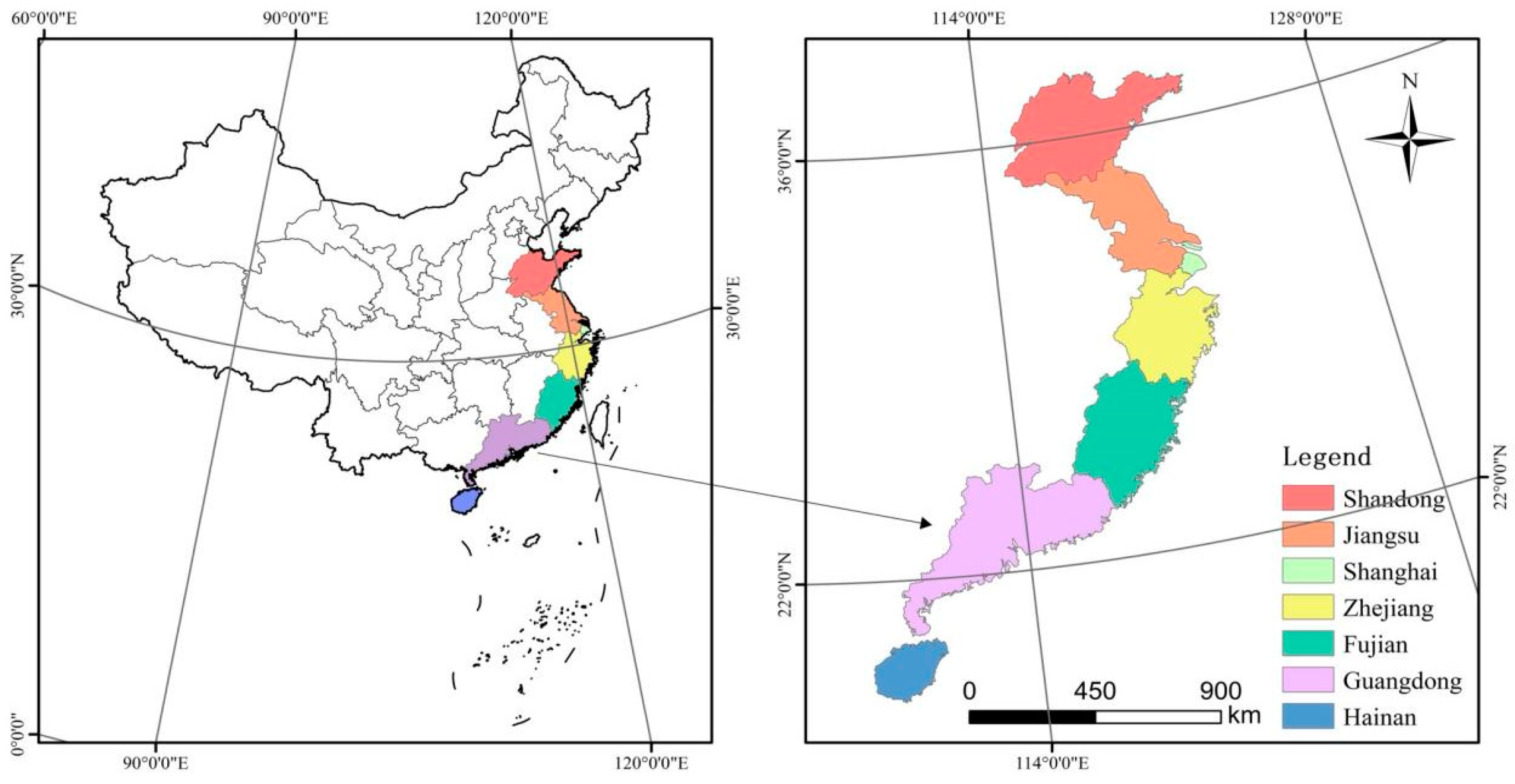
3.1. Research Area

The scope of this paper encompasses seven eastern coastal provinces and cities: namely, Hainan Province, Guangdong Province, Fujian Province, Zhejiang Province, Jiangsu Province, Shanghai Municipality and Shandong Province. Notably, the Shanghai Municipality is treated as a distinct study unit due to its significant economic, demographic and carbon emission characteristics. Situated in the eastern coastal area of mainland China, this region experiences a humid climate and is endowed with abundant natural resources. It plays a crucial role in national ecological security, serving as a key component of the “Maritime Silk Road” and holding a pivotal position in economic and social development and sustainable construction. As of 2023, the research area spans approximately 700,000 square kilometers, accommodating a total population of approximately 452,790,000 people. The construction industry, a major economic contributor, engages more than 20 million individuals, with a total output value surpassing USD 1 billion. The swift expansion of industrial development and housing demand has led to the rapid growth of the construction sector in this region. Consequently, substantial carbon emissions contribute to environmental pollution, ecological degradation and issues such as wetland shrinkage. In light of these challenges, the paper focuses on a comprehensive study of Hainan Province, Guangdong Province, Fujian Province, Zhejiang Province, Jiangsu Province, Shanghai Municipality and Shandong Province. These six provinces and one municipality constitute the primary study area, as illustrated in Figure 1.

3.2. Data Processing

3.2.1. Min–Max Normalization Method

Before starting model training, the original dataset underwent normalization. Various normalization techniques are available, such as min–max normalization, Z-score normalization, robust normalization, sigmoid normalization, Principal Component Analysis (PCA) and others. In this study, we opted for the min–max normalization method to rescale the original data into the [0, 1] interval. The functional expression representing this approach is depicted in Equation (1):

$$X_{1(\mathrm{normalized})}=\frac{X_1-X_{1(\mathrm{Min})}}{X_{1\left(\mathrm{Max}\right)}-X_{1(\mathrm{Min})}}(\mathrm{Max}-\mathrm{Min})+\mathrm{Min}$$

(1)

where $X_{1(\mathrm{normalized})}$ represents the normalized sample data, $X_1$ signifies the original sample data, $X_{1(\mathrm{Max})}$ is the maximum value within the sample data and $X_{1(\mathrm{Min})}$ is the minimum value within the sample data. The terms “max” and “min” denote the maximum and minimum values after normalization, conventionally set to 1 and 0, respectively. In this study, we adopted the values of max = 1 and min = 0.

3.2.2. Fixed-Effects Model

The fixed-effects model is a statistical model used to study differences among objects or entities that have some unchanging unique characteristics over a period of time. These characteristics can be natural resources, geographical location and climate conditions, etc., which can affect carbon emissions. In fact, these characteristics can be very important determinants of carbon emissions, so any model trying to predict or explain carbon emissions needs to take these factors into account. However, in many cases, these variables are difficult to measure or directly observe. In the fixed-effects model, each entity or object (province) is assigned a fixed effect that represents factors we cannot observe or measure.

This can eliminate the bias that these unobserved inherent variables may bring. More specifically, it can accurately capture the impact of changes in the variables we can observe and measure over time on carbon emissions, because the unobserved factors have been fixed. In this study, through introducing the fixed effect of each province, it can capture the unique characteristics of each province that do not easily change during the study, such as natural resources, geographical location and so on. This can provide a more accurate view of the relationship between changes in the carbon emissions of different provinces and other explanatory variables, improving the predictive accuracy of the model. The calculation expression of the individual fixed-effect coefficient is as shown in Equation (2):

$${\widehat{\alpha }}_i={\overline{y}}_i-{{\overline{x}}_i}^T\widehat{\beta }$$

(2)

In the equation, ${\widehat{\alpha }}_i$ represents the individual fixed-effect coefficient of the ith province, ${\overline{y}}_i$ denotes the average carbon emission value from the construction industry in the ith province spanning the years 2005 to 2020, ${\overline{X}}_i$ signifies the average value of 11 explanatory variables in the ith province and $\widehat{\beta }$ corresponds to the least-squares estimation of the fixed-effect coefficients in the mixed-effects model. The implementation of this model was carried out using the Statsmodels library in Python.

4. Research Approach and Methodology

4.1. Research Approach

This study focuses on seven coastal provinces and cities in eastern China, using panel data from 2000 to 2020 as the dataset. There were three research stages, namely, data processing, influential factor selection and predictive model comparison. Considering both prediction accuracy and effectiveness, the BO-XGBoost model, which exhibits high prediction accuracy and strong global search capability, was identified as the most suitable model. The specific theoretical framework is illustrated in Figure 2.

4.2. Accounting for CECI

Carbon emissions originating from the construction industry emanate from two primary sources [29]. First, direct carbon emissions encompass the release of carbon from the consumption of energy sources, such as coal, gasoline, oil, natural gas and electricity during the production activities of the construction industry. Second, indirect carbon emissions arise from the production and utilization of building materials commonly employed in the construction sector, including but not limited to cement, steel, wood, glass, aluminum and others. In accordance with the IPCC carbon emission-calculation formula, the expression for carbon emissions from the construction industry is presented by Equation (3):

$$E=E_{\mathrm{dir}}+E_{\mathrm{ind}}=\frac{44}{12}{\displaystyle \sum C_{\mathrm{i}}\times a_i+{\displaystyle \sum M_j\times {\beta }_j\times (1-{\epsilon }_j)}}$$

(3)

where $E_{\mathrm{dir}}$ represents the direct carbon emissions; $E_{\mathrm{ind}}$ denotes the indirect carbon emissions; $C_{\mathrm{i}}$ refers to the ith type of energy consumption; ${\alpha }_i$ signifies the carbon emission coefficient of the ith type of energy; $M_j$ represents the utilization of the jth type of building materials in the construction industry; ${\beta }_j$ stands for the carbon emission coefficient of the jth type of building materials; and ${\epsilon }_j$ denotes the recycling coefficient of the jth type of building materials. For steel, the recovery coefficient is 0.80, for aluminum, the recovery coefficient is 0.85 and for all other types of building materials, the recovery coefficient is 0 [30]. The specific carbon emission coefficients and building materials are detailed in

Table 1. Conversion factors of carbon emissions from various energy sources.

Types of Energy	Lower Heating Value *	Carbon Content Per Unit Calorific Value *	Carbon Oxidation Rate *
Raw coal	20.908	25.800	0.899
Washed anthracite	26.344	25.800	0.899
Other washed coal	9.409	25.800	0.899
Shaped coal	16.800	25.800	0.899
Coke	28.435	29.200	0.970
Coke oven gas	17.981	12.100	0.990
Other coal gas	8.429	12.100	0.990
Crude oil	41.816	20.000	0.980
Gasoline	43.070	18.900	0.980
Kerosene	43.070	19.500	0.980
Diesel	42.625	20.200	0.980
Liquefied petroleum gas	50.179	17.200	0.990
Fuel oil	41.816	21.100	0.980
Refinery dry gas	45.998	15.700	0.990
Natural gas	38.931	15.300	0.990
Other petroleum products	40.190	20.000	0.980
Other coking products	28.435	29.200	0.970

* The data in Table 1 come from the research of Fan J S [31]. https://www.resci.cn/EN/10.18402/resci.2019.05.07, accessed on 1 May 2023.

and

Table 2. CO₂ emission factors of building materials.

Types of Materials	Steel	Wood	Cement	Glass	Aluminum
Carbon dioxide emission factor *	1.79	−842.80	0.82	0.97	2.60
Recycling rate *	0.80	0.00	0.00	0.00	0.85

* The data in Table 2 come from the research of Chi Y [32]. https://doi.org/10.3390/su13041876, accessed on 1 May 2023.

.

4.3. Preliminary Selection of Influencing Factors on CECI

The CECI are influenced by various factors across distinct domains. Drawing from the existing research, we categorized these influencing factors into four groups, as detailed in

Table 3. Categories of factors influencing the construction industry’s CO₂ emissions.

Category	Influencing Factors	Abbreviation	Reference Literature
Population factors	Total Population	TP	[33]
	Employment in the Construction Industry	ECI	[34,35,36]
Economic factors	Gross Domestic Product	GDP	[34]
	Urbanization Rate	UR	[34,36,37]
Technological factors	Floor Space of Buildings Completed	FSB	[38]
	Total Output of the Construction Industry	TOC *	[34,36]
	Standard Of Living	SL *	[39]
	Industrial Structure	IS *	[34,40,41]
	Energy Emission Intensity	EEI *	[37,41]
	Labor Productivity in the Construction Industry	LPC	[34]
	Technological Equipment Rate of Construction Enterprises	TEC	[36,42]
Geographic factors	Provincial Disparities	PD *	[43]

* SL represents the consumer price index; IS represents the ratio of the TOC to the GDP; EEI represents the ratio of the construction industry’s energy consumption in terms of standard coal to the TOC; PD is derived from Formula (2); the rest were obtained directly from various yearbooks.

: demographic factors, economic factors, technological factors and geographic factors. Demographic factors include the total regional population and employment in the construction industry. Economic factors encompass the GDP and urbanization rate. Technical factors include the floor space of buildings completed; the total output of the construction industry; the standard of living; the industrial structure, energy emission intensity and labor productivity in the construction industry; and the technical equipment rate of construction enterprises. Geographic factors are identified based on provincial disparities. Specifically, the standard of living is characterized by the consumer price index, the industrial structure is defined by the ratio of the total output of the construction industry to GDP and the energy emission intensity is denoted by the ratio of CECI to the total output of the construction industry. Recognizing that inter-provincial variations significantly contribute to disparities in the CECI, we employed a fixed-effects model to quantify the differences among provinces as explanatory variables.

In this paper, numerous explanatory variables have been initially identified, each exerting different influences on the CECI. Some variables may exhibit low correlation with the final prediction outcomes. Therefore, in the process of forecasting carbon emissions from the construction industry, it is imperative to initially screen and analyze the selected explanatory variables. This step is crucial for enhancing the accuracy of the ultimate predictions. Given the intricate and non-linear nature of the relationship between explanatory variables and carbon emissions in the construction industry, the conventional Pearson correlation coefficient may not be the most suitable measure. Consequently, we opted to use the Spearman’s rank correlation coefficient to assess both the relationship between the 12 explanatory variables and CECI and the correlation among the 12 explanatory variables. Spearman’s rank correlation coefficients offer a more robust approach for capturing potential monotonic relationships, ensuring a comprehensive understanding of the intricate dynamics at play. The formula for Spearman’s rank correlation coefficient, Equation (4), is provided as follows:

$$R\mathrm{rank}=1-\frac{6{\displaystyle {\sum }_{i=1}^{\mathrm{n}}{D}^2}}{n(n^2-1)}$$

(4)

where D is the difference in rank between each pair of data, and n denotes the sample data.

4.4. Methods for Predicting CECI

This article compares RF, XGBoost with default parameters, XGBoost optimized by Grid Search (GS-XGBoost) and BO-XGBoost. Through comparing the default XGBoost with RF, we identified which algorithm was more suitable for the subject of this study. Additionally, through comparing GS-XGBoost and BO-XGBoost, we verified which optimization method produced better results.

4.4.1. XGBoost Algorithm

XGBoost, an integrated decision tree-based learning algorithm introduced by Chen [23] in 2016, constructs a new decision tree in each iteration by iteratively adding base learners. This iterative process aims to minimize the errors carried over from the previous models. Specifically, with each iteration, XGBoost updates the sample weights based on the residuals of the preceding model and trains a new decision tree using these adjusted weights. Through incorporating techniques such as regularization and tree pruning, XGBoost effectively mitigates the risk of overfitting, enhancing the model’s generalization capability beyond that of the traditional gradient boosting algorithm. This strategy not only corrects errors but also contributes to the overall robustness of the model. The introduction of regularization and tree pruning is pivotal in preventing the algorithm from memorizing the training data, promoting a more balanced and applicable model. The formula underpinning this process is expressed as follows:

$$obj(\theta )=\sum l(y_i,{\widehat{y}}_i)+\sum \Omega (f_k)$$

(5)

$$l(y_i,{\widehat{y}}_i)=\left|y_i-{\widehat{y}}_i\right|$$

(6)

$$\Omega \left(f\right)={\gamma }_{\gamma }+\frac{1}{2}\lambda {{\displaystyle \sum w_j}}^2$$

(7)

where $l(y_i,{\widehat{y}}_i)$ is the loss function, which is used to measure the error between the predicted and actual values of the CECI. is the regularization term, which is used to control the complexity of the model to prevent overfitting and consists of the number of leaf nodes T of the tree and the L2 norm of the leaf node scores; $\gamma$ is the complexity parameter controlling the number of leaf nodes on the tree; λ is the complexity parameter controlling the number of L2 norms of the leaf node scores; $w_j$ is the score of the jth leaf node; $y_i$ is the actual value of the CECI; ${\widehat{y}}_i$ is the predicted value of the CECI for the ith sample in the model; and $f_k$ is the kth tree in the model. In the learning process of the model, XGBoost adopts the gradient boosting method, and for each step, it adds a new tree to minimize the objective function. This added tree will cause the loss function to decrease the fastest. The form of adding a new tree is represented by Equation (8):

$$\stackrel{\wedge }{{\displaystyle y_i(t)}}={\displaystyle y_i(\stackrel{\wedge }{t}-1)}+\eta \times f_t(x_i)$$

(8)

In the given expression, $\eta$ denotes the learning rate, governing the magnitude of updates at each step, while $x_i$ represents the feature vector of the ith sample. It is noteworthy that both $f_k$ and $f_t$ pertain to a tree within the model, where $f_k$ is the kth tree in the model, and $f_t$ is the new tree added to the model at step t of the gradient boosting process. In this study, the prediction model was implemented using the Scikit-Learn and XGBoost machine learning libraries in Python.

4.4.2. Bayesian Optimization Algorithm

Bayesian Optimization (BO) is a global optimization algorithm grounded in probability distribution [14], with its algorithm primarily bifurcated into two integral components: the a priori function and the collection function. The a priori function harnesses Gaussian Process Regression (GPR), a non-parametric model constituting a set of random variables dictated by mean and covariance functions. Meanwhile, the collection function employs the Probability of Improvement (PI) criterion, steering the selection of the subsequent evaluation point within a hyperparametric decision space. In the context of optimizing the hyperparameters for the XGBoost carbon emission-prediction model within the construction industry, a hyperparameter sample dataset D = (X, y) is established. Here, X = (,…,) and y = {,…,} represent sets of continuous functions. In the process of making decisions about a set of hyperparameters, Bayesian optimization constructs a probabilistic model for the target function to be optimized. This model is then utilized to strategically choose the next evaluation point. Subsequently, the optimal solution for the hyperparameters is attained through an iterative loop.

$$x^{*}=\arg \min x_{\chi \in R^d}f(x)$$

(9)

where $x^{*}$ is the optimal hyperparameter combination, $\chi$ is the decision space, and $f(x)$ is the objective function.

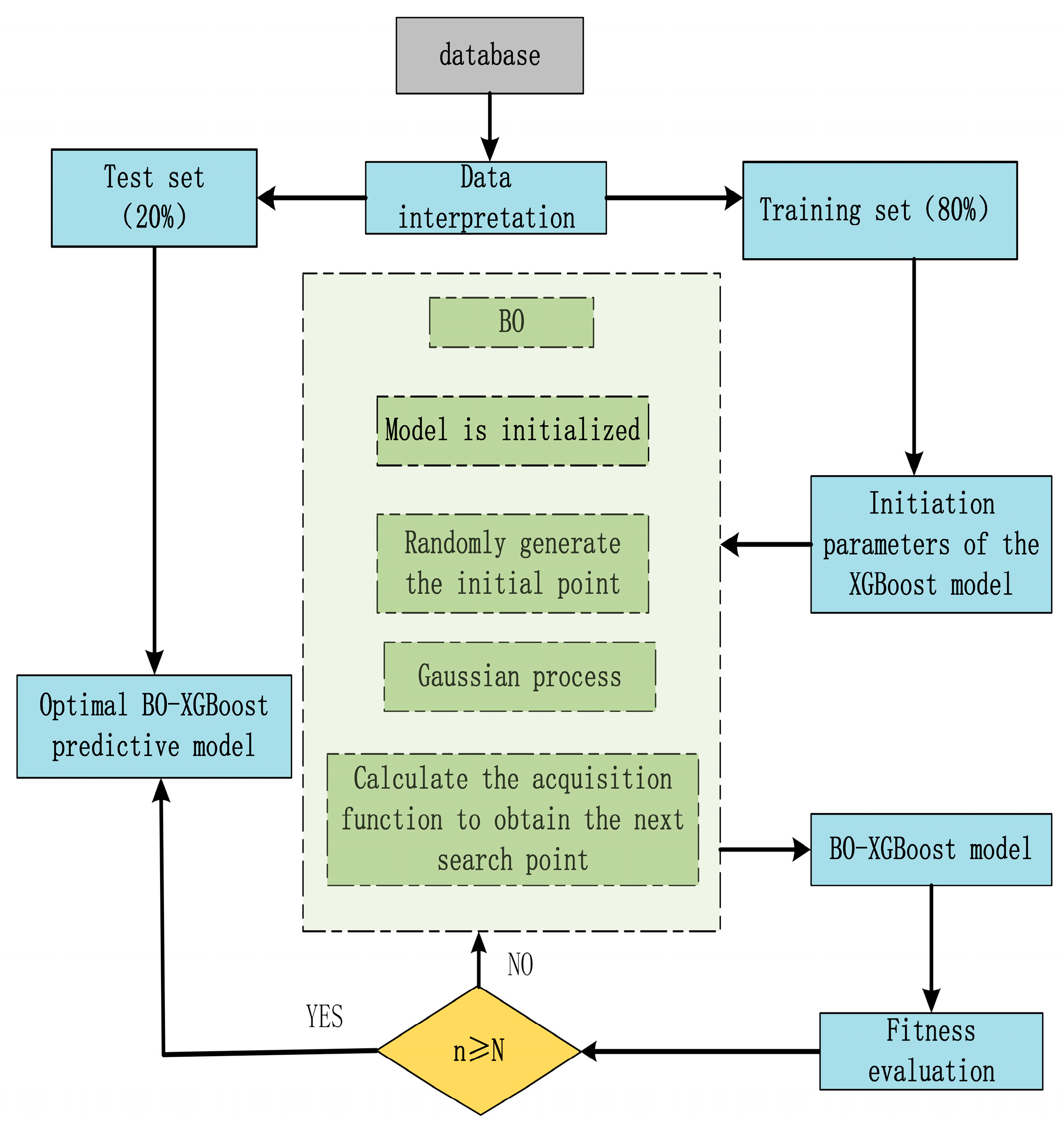
4.4.3. BO-XGBoost Model

A fusion of the Bayesian and XGBoost networks is employed to seek the optimal combination of parameters of the XGBoost model using Bayesian Optimization (BO). BO calculates the gain function based on the mean and variance of the objective function corresponding to the current search point. It iteratively adds a new hyperparameter search point with the maximum gain function to the set of evaluation points and updates the probabilistic agent model with this new set until the predetermined number of iterations is reached, ultimately yielding the optimal hyperparameter combination for XGBoost. The proposed hyperparameter optimization method is integrated seamlessly into the model training process, as opposed to being confined to the model testing phase. The training data are introduced into the network, and the model is trained using the designated network parameters. Feedback is derived from the loss function values of the validation data, steering continuous adjustments to the model parameters. Ultimately, the model parameters associated with the highest accuracy in the training set are extracted and output. Subsequently, the test set data are fed into the trained model for testing, and the accuracy of the test set is determined. The dataset used in this study had a total of 112 entries, which were divided into a training set (89 entries, 80%) and a test set (23 entries, 20%). The detailed process is illustrated in Figure 3.

Configuring the XGBoost model involves a multitude of parameters, and their interdependence renders manual and iterative parameter tuning impractical for effective model training comparisons. Consequently, the Bayesian algorithm emerges as a viable solution to iteratively determine the optimal hyperparameter configuration for the XGBoost model.

4.4.4. Evaluation Indicators for Prediction Models

In this study, we selected four prominent metrics widely employed in the literature to assess the performance of the four models. These metrics encompass the Root Mean Square Error (RMSE), the Mean Absolute Error (MAE), the Coefficient of Determination (R2) and the Mean Absolute Percentage Error (MAPE).

$$RMSE=\sqrt{\frac{1}{N}{\displaystyle {\sum }_{i=1}^n{X}_p-{X_o}^2}}$$

(10)

$$MAE=\frac{1}{N}{\displaystyle {\sum }_{i=1}^n{X}_p-X_o}$$

(11)

$$R^2=\frac{{\displaystyle {\sum }_{i=1}^N{X}_0-{\overline{X}}_0{X}_p-{\overline{X}}_p}}{\sqrt{{\displaystyle {\sum }_{i=1}^N{X}_0-{\overline{X}}_0^2{\displaystyle {\sum }_{i=1}^N{X}_p-{\overline{X}}_p}}}}$$

(12)

$$MAPE=\frac{1}{N}{\displaystyle \sum _{\mathrm{i}=1}^N\left|\frac{X_p-X_0}{X_0}\right|}$$

(13)

where $X_p$, $X_0$, ${\overline{X}}_p$ and ${\overline{X}}_0$ denote the predicted, observed, average predicted and average observed values, respectively.

5. Results and Analysis

5.1. Measurement of Carbon Emissions from the Construction Industry

Figure 4 illustrates the CECI and their trends in seven provinces and cities for the years 2005, 2010, 2015 and 2020. Overall, the CECI in the seven provinces and cities exhibited an upward trend, increasing from 310 million tons in 2005 to 1.72 billion tons in 2020. From the perspective of CECI, it was determined that from 2005 to 2020, the total carbon emissions of seven provinces and cities each year amounted to approximately 1.529 billion tons. The total direct carbon emissions accounted for around 444 million tons, approximately 29% of the total carbon emissions. The indirect carbon emissions summed up to about 1.084 billion tons, approximately 71% of the total carbon emissions. Further analysis revealed varying contributions of different energy sources and building materials to carbon emissions. In direct carbon emissions, coal and petroleum products were found to be the most notable contributors. Conversely, in indirect carbon emissions, steel and cement accounted for the highest contribution through their consumption. Therefore, a significant reduction in the carbon emissions of the construction industry can be achieved by minimizing the overuse and wastage of these materials.

During the study period, Shandong Province topped the list for carbon emissions, followed by Zhejiang and Jiangsu Provinces, while Hainan Province emitted the least. The high carbon emissions in Shandong could primarily be attributed to its coal-centric industrial and energy structures. Industries such as steel and building materials, which are prevalent in Shandong and known for their low energy efficiency, rely heavily on coal, thereby resulting in high carbon dioxide emissions.

Shanghai managed to maintain steady, slow growth in its construction industry emissions throughout the duration of the study, even preserving a relatively low carbon emission level in 2020. Shanghai’s success in this regard could largely be attributed to its commitment to energy conservation and emission reduction as a significant economic hub, both in China and worldwide. This commitment is reflected in the city’s introduction of parliament policies, including stringent monitoring of construction processes, strict prohibition against inferior construction materials and techniques and the promotion of green construction. The latter policy presents the participation and assembly rates for prefabricated structures as project-acceptance criteria. These low carbon-supporting policies have contributed to keeping Shanghai’s increase rate in construction industry carbon emissions within an acceptable range.

5.2. Results of Factors Influencing CECI

To rigorously examine the quantitative relationship between the 12 explanatory variables and the carbon emissions originating from the construction industry, this study employed the dataset to initially compute the individual fixed-effect coefficients for each province (PD). Subsequently, the Spearman’s rank correlation coefficient method was employed to assess the correlation coefficients between the 12 explanatory variables and the emissions from the construction industry. In tandem with a significance test, this aided in the meticulous screening of the explanatory variables. The correlation coefficients, along with their corresponding rankings, are visually presented in Figure 5.

In the figure, red is significant, and gray is not. The ECI-SL correspondingly denote the following: employment in the construction industry, floor space of buildings completed, total output of the construction industry, industrial structure, gross domestic product, total population, energy emission intensity, urbanization rate, labor productivity in the construction industry, provincial disparities, technological equipment rate of construction enterprise and standard of living.

Eight of the initially selected explanatory variables successfully passed the 0.01 two-sided significance test, indicating a robust correlation with the explanatory variables. Notably, ECI, FSB and TOC exhibited stronger correlations. This is attributed to their inherent direct relationship with the generation of CECI, allowing them to more directly influence the CECI. Additionally, the heterogeneity among provinces quantified by a fixed-effects model also can significantly influence the CECI.

Four variables—namely, UR, SL, TEC and LPC—do not meet the significance test criteria. The possible reason for this is that these factors more intricately reflect the fundamental features and characteristics of the construction system. The relationship with CECI is therefore more complex, making it challenging for these variables to directly reflect the carbon emissions of the construction industry. Thus, the correlation between these factors and CECI may be relatively weak.

After computing the correlation between the explanatory variables and carbon emissions, it was essential to assess the correlation among the explanatory variables to mitigate the impact of multicollinearity, a factor that can compromise the model’s accuracy. Generally, a correlation coefficient exceeding 0.7 signifies a very close relationship, while a coefficient ranging from 0.4 to 0.7 indicates a close relationship. Furthermore, a coefficient falling between 0.2 and 0.4 suggests an average relationship. Therefore, this study established a threshold at 0.4. As shown in Figure 6, it is evident that the Spearman correlation coefficients for all variables do not exceed 0.4. Consequently, this study used these eight explanatory variables as the input variables and the CECI as the output variable of the model.

5.3. Comparison and Validation of Carbon Emission-Prediction Models

The dataset, comprising panel data from seven provinces and cities spanning 2005 to 2020, was partitioned into a training set and a test set, with the proportions set at 80% (89 entries) and 20% (23 entries), respectively. Multiple tests were conducted to define the hyperparameter combinations for XGBoost within the optimization range. Subsequently, Bayesian optimization, complemented by cross-validation, was applied to fine-tune the XGBoost algorithm’s hyperparameters.

Table 4. Search space and optimal hyperparameters.

Model Parameters	Parameter Explanation
max_depth	Limiting the maximum depth of a tree	(3,9)	4
gamma	Penalty term coefficient, the minimum loss	(0,1)	1
min_child_weight	Minimum leaf node sample to split the node	(0,1)	0.119
reg_alpha	L1 regularization parameters	(0,1)	1
n_estimators	Number of iterations raised	(100,200)	193

presents the essential details, including the meanings of the key tuning parameters, the optimization parameter range and the conclusive results of the optimization search.

To delve deeper into the comparison of predictive capabilities among the BO-XGBoost, GS-XGBoost, XGBoost with default parameters and the Random Forest model, Figure 7 showcases the regression plots of these models during the testing stage. In this illustration, the horizontal axis represents actual carbon emissions, while the vertical axis portrays the predicted values generated by the models. The data points aligning with the red diagonal signify instances where the predicted values match the actual ones. Thus, the closer these points cluster to the red diagonal, the more accurate the predictive performance of the model. Notably, the predicted values of all four models closely approximate the actual values, indicating high overall fitting performance. Among them, the BO-XGBoost model exhibited the most optimal fit.

It was essential to assess how the performance of the algorithms evolved before and after Bayesian network optimization. The evaluation metrics RMSE, MAE, ${\mathrm{R}}^2$ and MAPE were employed to gauge the prediction performance of all models. The calculated results are summarized in Figure 8.

The RMSE represents the Root Mean Square Error, with smaller values indicating more stable prediction results. According to the measurement results, the stability of the XGBOOST algorithm predictions surpasses that of the Random Forest. Regarding the MAE, denoting the Mean Absolute Error, BO-XGBoost outperformed the others. BO-XGBoost exhibited ${\mathrm{R}}^2$ values exceeding 0.8, signifying satisfactory results in predicting carbon emissions from the construction industry. The MAPE is as an indicator for assessing prediction performance, with lower values indicating better performance. BO-XGBoost attained the minimum MAPE value, indicating good prediction accuracy. Considering all four indicators collectively, BO-XGBoost, constructed based on the BO-XGBOOST algorithm, demonstrated the most effective prediction.

In order to more intuitively reflect the performance of each model, control tests were conducted using the default hyperparameter XGBoost model, GS-XGBoost and the Random Forest model. Figure 9 presents a comparison between the predicted values and the actual values. It is apparent that the BO-XGBoost demonstrated superior regression performance and higher prediction accuracy.

6. Conclusions and Recommendations

6.1. Conclusions

(1)

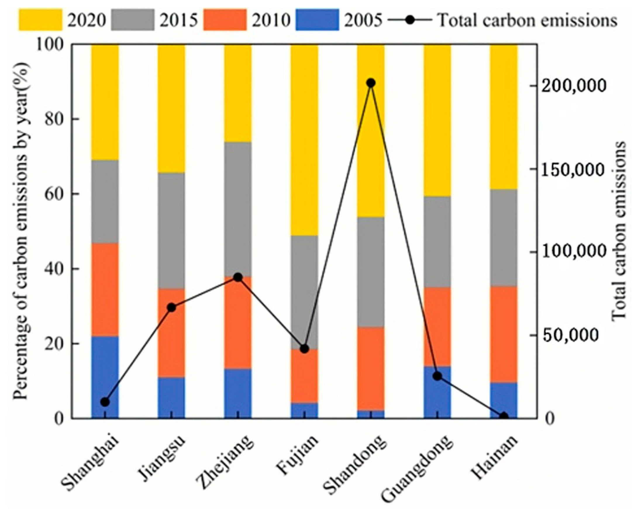
According to the IPCC emission factor method, spanning the years 2005 to 2020, the cumulative carbon emissions from the construction industry in the seven provinces and municipalities under scrutiny exhibited an escalating trend, surging from 310 million tons to 1.72 billion tons. Among the individual provinces and municipalities, Shandong Province emerged as the foremost emitter of carbon emissions from the construction sector, while Hainan Province registered the lowest emissions.

(2)

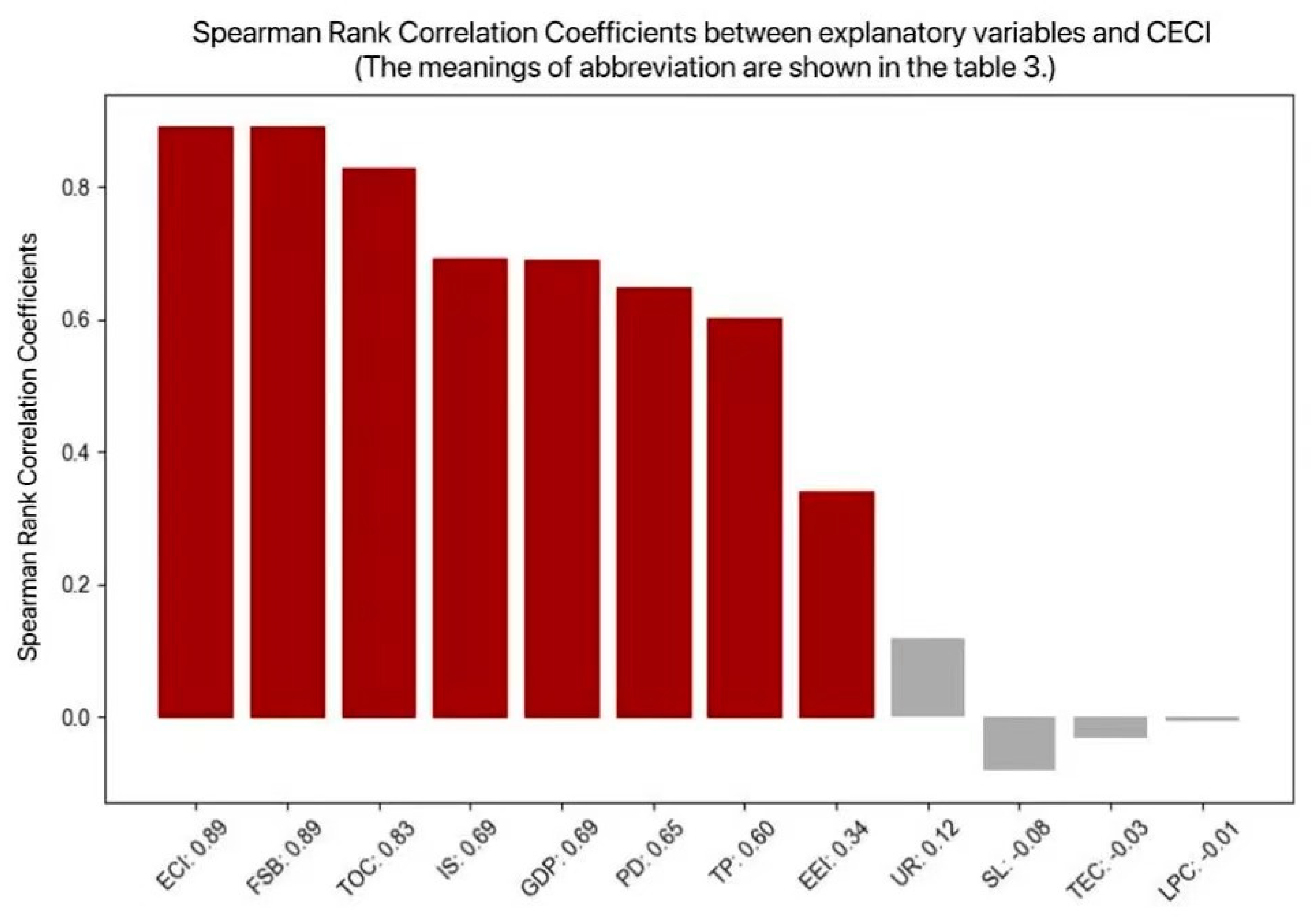
In reviewing the 12 factors influencing carbon emissions, 8 of them exhibited strong correlations with the CECI. These factors include employment in the construction industry, the floor space of buildings completed, the total output of the construction industry, industrial structure, gross domestic product, provincial disparities, the total population and the energy emission intensity. Meanwhile, it should be noted that the disparities among provinces should not be overlooked by researchers studying regional carbon emissions.

(3)

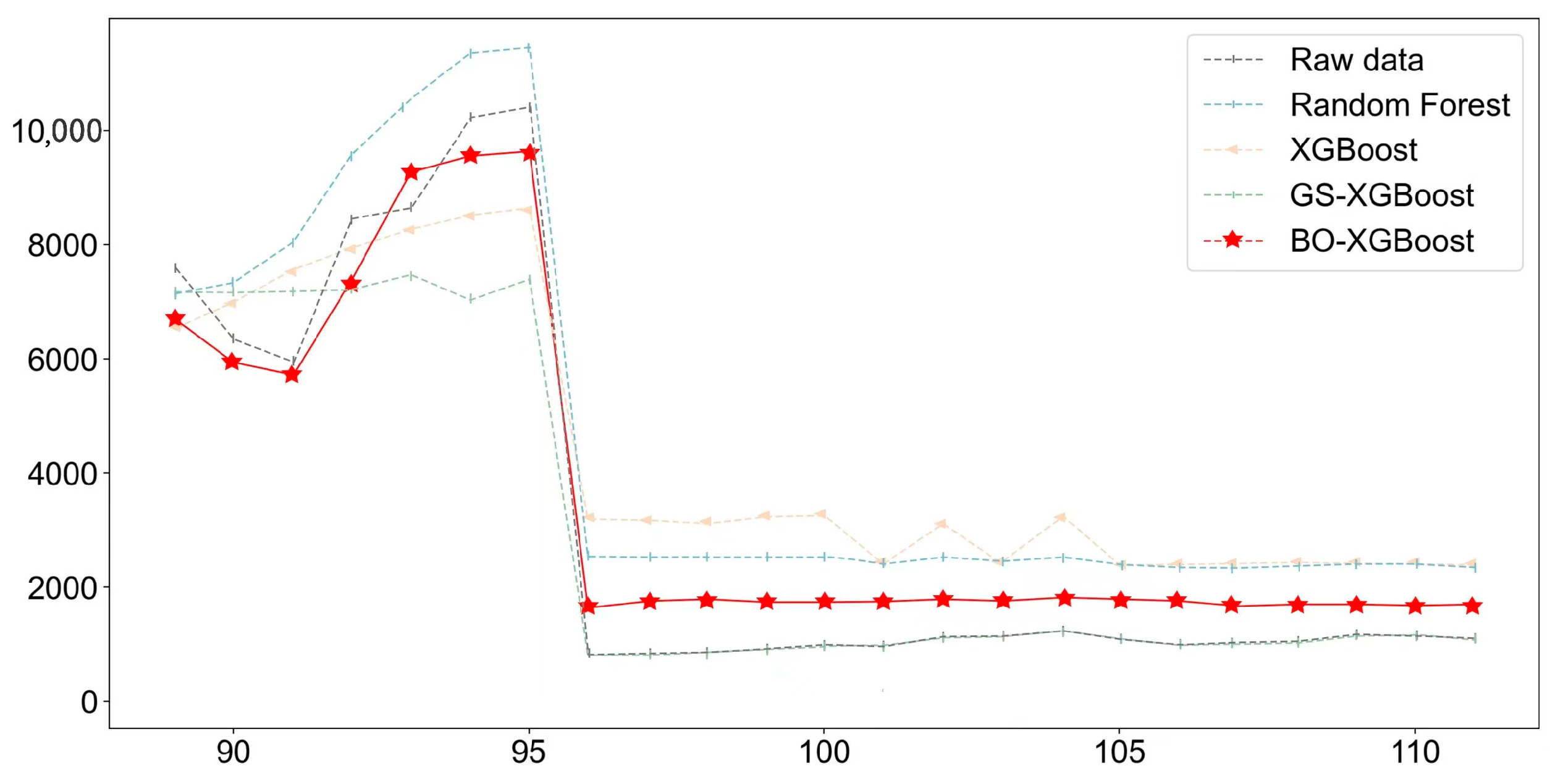
The Random Forest, XGBoost, BO-XGBoost and GS-XGBoost algorithms demonstrated commendable performance in fitting both the training and test sets. Notably, considering the four indicators of RMSE, MAE, $R^2$ and MAPE for validation, it was concluded that the BO-XGBoost model is more suitable for predicting carbon dioxide emissions in the construction industry.

6.2. Policy Recommendations

Based on the results of carbon emission accounting, the analysis of carbon emission influencing factors and prediction research, the following policy suggestions are proposed:

(1)

The demand to optimize the energy structure is vital. Currently, the main energy consumption in the construction industry comes from fossil fuels, primarily coal. The primary way to achieve carbon emission reduction involves controlling the total energy consumption and optimizing the consumption structure. It is necessary to strongly promote green energy sources, such as solar, wind and electricity, and establish a complementary multi-energy supply and utilization system. At the same time, we need to enhance the sustainable and efficient use of traditional energy sources, such as coal.

(2)

To address carbon emissions at their source, we must reduce energy consumption in the production of building materials. At present, the indirect carbon emissions from the construction industry primarily come from steel, timber and cement. Therefore, we need to both use these materials wisely and change the production processes of building materials, developing material transformation technology that turns waste materials into usable new materials and can reduce our reliance on raw resources, subsequently lowering carbon emissions.

(3)

Based on the analysis of the influencing factors of carbon emissions, the number of employees in the construction industry, the amount of completed construction area, the total output value and provincial disparities all have a strong correlation with carbon emissions. Therefore, we need to formulate policies based on local conditions, such as elevating employee skills through training and education to better meet environmental standards. It is worth noting that the government should establish a carbon emissions trading market or implement a carbon tax system to tax construction companies with higher carbon emissions, incentivizing them to reduce their emissions and improve productivity and energy efficiency.

References

- Li, D.; Huang, G.; Zhu, S.; Chen, L.; Wang, J. How to peak carbon emissions of provincial construction industry? Scenario analysis of Jiangsu Province. Renew. Sustain. Energy Rev. 2021, 144, 110953. [Google Scholar] [CrossRef]
- Pu, X.; Yao, J.; Zheng, R. Forecast of energy consumption and carbon emissions in China’s building sector to 2060. Energies 2022, 15, 4950. [Google Scholar] [CrossRef]
- Wakiyama, T.; Kuramochi, T. Scenario analysis of energy saving and CO2 emissions reduction potentials to ratchet up Japanese mitigation target in 2030 in the residential sector. Energy Policy 2017, 103, 1–15. [Google Scholar] [CrossRef]
- Huang, L.; Krigsvoll, G.; Johansen, F.; Liu, Y.; Zhang, X. Carbon emission of global construction sector. Renew. Sustain. Energy Rev. 2018, 81, 1906–1916. [Google Scholar] [CrossRef]
- Onat, N.C.; Kucukvar, M. Carbon footprint of construction industry: A global review and supply chain analysis. Renew. Sustain. Energy Rev. 2020, 124, 109783. [Google Scholar] [CrossRef]
- Guo, X.; Fang, C. Spatio-temporal interaction heterogeneity and driving factors of carbon emissions from the construction industry in China. Environ. Sci. Pollut. Res. 2023, 30, 81966–81983. [Google Scholar] [CrossRef] [PubMed]
- Atmaca, A.; Atmaca, N. Life cycle energy (LCEA) and carbon dioxide emissions (LCCO2A) assessment of two residential buildings in Gaziantep, Turkey. Energy Build. 2015, 102, 417–431. [Google Scholar] [CrossRef]
- Li, D.; Huang, G.; Zhang, G.; Wang, J. Driving factors of total carbon emissions from the construction industry in Jiangsu Province, China. J. Clean. Prod. 2020, 276, 123179. [Google Scholar] [CrossRef]
- Ma, M.; Cai, W. Do commercial building sector-derived carbon emissions decouple from the economic growth in Tertiary Industry? A case study of four municipalities in China. Sci. Total Environ. 2019, 650, 822–834. [Google Scholar] [CrossRef]
- Hung, C.C.; Hsu, S.-C.; Cheng, K.-L. Quantifying city-scale carbon emissions of the construction sector based on multi-regional input-output analysis. Resour. Conserv. Recycl. 2019, 149, 75–85. [Google Scholar] [CrossRef]
- Liu, B.; Wang, D.; Xu, Y.; Liu, C.; Luther, M. Embodied energy consumption of the construction industry and its international trade using multi-regional input–output analysis. Energy Build. 2018, 173, 489–501. [Google Scholar] [CrossRef]
- Wu, Y.; Chau, K.; Lu, W.; Shen, L.; Shuai, C.; Chen, J. Decoupling relationship between economic output and carbon emission in the Chinese construction industry. Environ. Impact Assess. Rev. 2018, 71, 60–69. [Google Scholar] [CrossRef]
- Jiang, T.; Huang, S.; Yang, J. Structural carbon emissions from industry and energy systems in China: An input-output analysis. J. Clean. Prod. 2019, 240, 118116. [Google Scholar] [CrossRef]
- Zheng, L.; Mueller, M.; Luo, C.; Menneer, T.; Yan, X. Variations in whole-life carbon emissions of similar buildings in proximity: An analysis of 145 residential properties in Cornwall, UK. Energy Build. 2023, 296, 113387. [Google Scholar] [CrossRef]
- Du, Q.; Lu, X.; Li, Y.; Wu, M.; Bai, L.; Yu, M. Carbon emissions in China’s construction industry: Calculations, factors and regions. Int. J. Environ. Res. Public Health 2018, 15, 1220. [Google Scholar] [CrossRef]
- Zhao, Y.; Duan, X.; Yu, M. Calculating carbon emissions and selecting carbon peak scheme for infrastructure construction in Liaoning Province, China. J. Clean. Prod. 2023, 420, 138396. [Google Scholar] [CrossRef]
- Zhang, C.-Y.; Zhao, L.; Zhang, H.; Chen, M.-N.; Fang, R.-Y.; Yao, Y.; Zhang, Q.-P.; Wang, Q. Spatial-temporal characteristics of carbon emissions from land use change in Yellow River Delta region, China. Ecol. Indic. 2022, 136, 108623. [Google Scholar] [CrossRef]
- Abdullah, L.; Pauzi, H.M. Methods in forecasting carbon dioxide emissions: A decade review. J. Teknol. 2015, 75, 67–82. [Google Scholar] [CrossRef]
- Lü, X.; Lu, T.; Kibert, C.J.; Viljanen, M. Modeling and forecasting energy consumption for heterogeneous buildings using a physical–statistical approach. Appl. Energy 2015, 144, 261–275. [Google Scholar] [CrossRef]
- Zubair, M.U.; Ali, M.; Khan, M.A.; Khan, A.; Hassan, M.U.; Tanoli, W.A. BIM-and GIS-Based Life-Cycle-Assessment Framework for Enhancing Eco Efficiency and Sustainability in the Construction Sector. Buildings 2024, 14, 360. [Google Scholar] [CrossRef]
- Yang, X.; Hu, M.; Wu, J.; Zhao, B. Building-information-modeling enabled life cycle assessment, a case study on carbon footprint accounting for a residential building in China. J. Clean. Prod. 2018, 183, 729–743. [Google Scholar] [CrossRef]
- Yan, S.; Zhang, Y.; Sun, H.; Wang, A. A real-time operational carbon emission prediction method for the early design stage of residential units based on a convolutional neural network: A case study in Beijing, China. J. Build. Eng. 2023, 75, 106994. [Google Scholar] [CrossRef]
- Wang, Q.; Li, S.; Pisarenko, Z. Modeling carbon emission trajectory of China, US and India. J. Clean. Prod. 2020, 258, 120723. [Google Scholar] [CrossRef]
- Jiang, W.; Yu, Q. Carbon emissions and economic growth in China: Based on mixed frequency VAR analysis. Renew. Sustain. Energy Rev. 2023, 183, 113500. [Google Scholar] [CrossRef]
- Pan, C.; Wang, H.; Guo, H.; Pan, H. How do the population structure changes of China affect carbon emissions? An empirical study based on ridge regression analysis. Sustainability 2021, 13, 3319. [Google Scholar] [CrossRef]
- Alabdullah, A.A.; Iqbal, M.; Zahid, M.; Khan, K.; Amin, M.N.; Jalal, F.E. Prediction of rapid chloride penetration resistance of metakaolin based high strength concrete using light GBM and XGBoost models by incorporating SHAP analysis. Constr. Build. Mater. 2022, 345, 128296. [Google Scholar] [CrossRef]
- Malkomes, G.; Schaff, C.; Garnett, R. Bayesian optimization for automated model selection. In Proceedings of the 30th Conference on Neural Information Processing Systems (NIPS 2016), Barcelona, Spain, 5–10 December 2016. [Google Scholar]
- Wu, J.; Chen, X.-Y.; Zhang, H.; Xiong, L.-D.; Lei, H.; Deng, S.-H. Hyperparameter optimization for machine learning models based on Bayesian optimization. J. Electron. Sci. Technol. 2019, 17, 26–40. [Google Scholar]
- Feng, B.; Wang, X.; Liu, B. Provincial variation in energy efficiency across China’s construction industry with carbon emission considered. Resour. Sci. 2014, 36, 1256–1266. [Google Scholar]
- Montes, C.; Kapelan, Z.; Saldarriaga, J. Predicting non-deposition sediment transport in sewer pipes using Random forest. Water Res. 2021, 189, 116639. [Google Scholar] [CrossRef]
- Fan, J.S.; Zhou, L. Spatiotemporal distribution and provincial contribution decomposition of carbon emissions for the construction industry in China. Resour. Sci. 2019, 41, 897–907. [Google Scholar] [CrossRef]
- Chi, Y.; Liu, Z.; Wang, X.; Zhang, Y.; Wei, F. Provincial CO2 emission measurement and analysis of the construction industry under China’s carbon neutrality target. Sustainability 2021, 13, 1876. [Google Scholar] [CrossRef]
- Zhou, W.; Yu, W. Regional variation in the carbon dioxide emission efficiency of construction industry in China: Based on the three-stage DEA model. Discret. Dyn. Nat. Soc. 2021, 2021, 1–13. [Google Scholar] [CrossRef]
- Dai, D.; Li, K.; Zhao, S.; Zhou, B. Research on prediction and realization path of carbon peak of construction industry based on EGM-BP model. Front. Energy Res. 2022, 10, 981097. [Google Scholar] [CrossRef]
- Yang, Z.; Fang, H.; Xue, X. Sustainable efficiency and CO2 reduction potential of China’s construction industry: Application of a three-stage virtual frontier SBM-DEA model. J. Asian Archit. Build. Eng. 2022, 21, 604–617. [Google Scholar] [CrossRef]
- Yang, J.; Zheng, X. The Spatiotemporal Distribution Characteristics and Driving Factors of Carbon Emissions in the Chinese Construction Industry. Buildings 2023, 13, 2808. [Google Scholar] [CrossRef]
- Chen, H.; Lu, C. Research on the Spatial Effect and Threshold Characteristics of New-Type Urbanization on Carbon Emissions in China’s Construction Industry. Sustainability 2023, 15, 15825. [Google Scholar] [CrossRef]
- Cong, X.; Zhao, M.; Li, L. Analysis of carbon dioxide emissions of buildings in different regions of China based on STIRPAT model. Procedia Eng. 2015, 121, 645–652. [Google Scholar] [CrossRef]
- Chun-Jing, S.; Jin, C.; Yan-Rong, L.; Wei-Zhi, L. Carbon emission accounting analysis and prediction research of construction industry in Hainan Province. Environ. Eng. 2016, 34, 161–165. [Google Scholar]
- Wang, Y.; Wu, X. Research on High-Quality Development Evaluation, Space–Time Characteristics and Driving Factors of China’s Construction Industry under Carbon Emission Constraints. Sustainability 2022, 14, 10729. [Google Scholar] [CrossRef]
- Tian, D.; Li, M.C.; Shi, J.; Shen, Y.; Han, S. On-site text classification and knowledge mining for large-scale projects construction by integrated intelligent approach. Adv. Eng. Inform. 2021, 49, 12. [Google Scholar] [CrossRef]
- Hui-tian, L.; Da-wei, H. Construction and Analysis of Machine Learning Based Transportation Carbon Emission Prediction Model. Environ. Sci. 2023, 44, 1–17. [Google Scholar] [CrossRef]
- Cheng, S.; Fan, W.; Meng, F.; Chen, J.; Liang, S.; Song, M.; Liu, G.; Casazza, M. Potential role of fiscal decentralization on interprovincial differences in CO2 emissions in China. Environ. Sci. Technol. 2020, 55, 813–822. [Google Scholar] [CrossRef]