A Point-Interval Forecasting Method for Wind Speed Using Improved Wild Horse Optimization Algorithm and Ensemble Learning

Abstract

With the implementation of the green development strategy and the “double carbon goal”, as an important energy for sustainable development, wind power has been widely researched and vigorously developed across the world. Wind speed prediction has a major impact on the grid dispatching of wind power connection. Most current studies only focus on the deterministic prediction of wind speed. However, the traditional deterministic forecast only provides the single wind speed prediction results and cannot meet the diverse demands of dispatchers. To bridge the gap, a wind speed point-interval forecasting method is proposed that utilizes empirical wavelet transform, an improved wild horse optimization algorithm, a multi-predictor, and improved kernel density estimation. This method decomposes the wind speed sequence into stationary subsequences through empirical wavelet transform, and then optimizes three basic learners with completely different learning mechanisms to form an ensemble model using the modified wild horse optimization algorithm. Finally, the uncertainty is analysed using an improved kernel density estimation. The datasets of three sites from America’s national renewable energy laboratory are used for comparison experiments with other models, and the predictions are discussed from different angles. The simulation results demonstrate that the model can produce high-precision deterministic results and high-quality probabilistic results. The reference information the model provides can be extremely valuable for scheduling operators.

1. Introduction

With the increasingly severe problems of traditional energy shortages and temperature warming, global energy transformation has become an important issue facing the world today. The global demand for clean energy is rising, particularly for renewables such as wind and solar, as the low-carbon energy transition is promoted [1,2]. According to the Global Wind Energy Council [3], up to 2022, the cumulative installed capacity worldwide is 906 GW, and China ranks first in the world both in terms of cumulative and newly installed capacity. However, because of the randomness and fluctuation of wind, with the increasing proportion of wind power in the power grid, the efficient consumption of wind power and the safe operation of the power system will face greater challenges [4]. Therefore, efficient and accurate wind resource assessment [5,6] and wind speed prediction research [7] are necessary conditions for reducing wind power development costs and maintaining the safe and stable operation of the power system. Wind resource assessment is mainly used for the site selection of wind farms in the early stage, while wind speed prediction provides guidance for power system scheduling after the wind farm is built. This article mainly studies the wind speed prediction of large wind farms.

To raise the wind speed forecasting precision, scholars have developed numerous effective models and have made significant contributions to wind power development. There are four groups of methods [8]: physical [9], statistical [10], intelligent [11], and hybrid [12]. Physical models rely on detailed geographic information and accurate meteorological data, which are computationally complex and commonly applied to long-term forecasting. Statistical methods utilize historical data analysis and modeling to predict future trends and results. Compared with physical methods, this method has the advantage of simple calculation. However, such methods require the collecting and processing of large amounts of historical data. Intelligent methods simplify modeling implementation by not requiring specific expressions between input and output. The Elman neural network (ENN) [13], least squares support vector machine (LSSVM) [14], back propagation neural network (BPNN) [15], and gate recurrent unit (GRU) [16] have all achieved good results for wind speed forecasting. The nonlinearity and uncertainty of wind speed sequences result in low prediction accuracy of intelligent models. Therefore, scholars have proposed hybrid models, which have become the most popular time series prediction structures due to their ability to fully integrate the advantages of data preprocessing, swarm intelligence optimization algorithms, and machine learning modules. Wu et al. [17] adopted complementary ensemble empirical mode decomposition (CEEMD) to preprocess wind speed series, and used an extreme learning machine (ELM) optimized by a multi-objective grey wolf optimization algorithm (MOGWO) to predict the decomposed wind speed subsequences. The results obtained good accuracy and stability. Ma et al. [18] employed CEEMD with adaptive noise (CEEMDAN) to process wind speed, and applied a long short-term memory network (LSTM) as a predictor to build prediction models for each subsequence. The resulting error sequence is decomposed by variational mode decomposition (VMD) using the same predictor for error correction. The results provide evidence that error correction can improve the forecasting accuracy. Krishna et al. [19] set up a wind power forecasting model using VMD and a hybrid kernel function ELM–autoencoder (MKELM-AE), in which VMD parameters were optimized by the sine cosine integrated water cycle algorithm (SCWCA). Compared to the comparison models, this model has obvious advantages.

Due to the limitations of each learner, prediction models based on one single learner may not always be applicable to all different research cases. An effective method to solve this problem is to integrate multiple base learners and construct a model with a stronger learning ability [20,21]. Wang et al. [22] constructed a multi-predictor ensemble model that reduced the wind speed dimension by fuzzy information particles, and optimized the weight coefficients of five models, namely BPNN, ELM, temporal convolutional network (TCN), GRU, and deep belief network (DBN) through a multi-objective dingo optimization algorithm (MODOA). The results show that this method outperforms the benchmark models in terms of forecasting precision and stability. Song et al. [23] established an integrated model using a meta-heuristic optimization algorithm, which utilized the grey wolf optimization algorithm (GWO) to obtain the weight coefficients of the predictors BPNN, ENN, wavelet neural network (WNN), and generalized neural network (GRNN). The results prove that the integrated model has a higher prediction accuracy and good universality for data with different features. Wei et al. [24] adopted Q-learning, a reinforcement learning technology, to weight GRU, outlier robust ELM (ORELM), and bidirectional LSTM (BiLSTM) on the basis of the error and reward mechanism, thereby achieving high-quality ship pitch point-interval prediction. Wang et al. [25] built an ensemble model for wind power prediction by taking partial least squares regression as an integration strategy. The results suggest that the ensemble model has high accuracy and adaptability. Although there is increasing research based on ensemble learning, there are still significant challenges in selecting basic learners and ensemble strategies.

At present, most research focuses only on deterministic prediction, which generates a single point prediction of future wind speeds, while ignoring the adverse effects of wind speed uncertainty on the power system. Different from point forecasting, probabilistic forecasting also provides uncertainty, that is, accurate estimation of the fluctuation range of the predicted wind speed, which provides more valuable reference information for the decision of the dispatcher [26,27,28]. The quantile regression neural network, which combines the advantages of a neural network and quantile regression, is often used in wind speed probabilistic forecasting [29,30]. However, this method requires separate modeling at each quantile, which increases the complexity of the model. Zhu et al. [31] combined Gaussian process regression with LSTM to achieve the probability prediction of wind speed. The results demonstrate that compared with the comparative model, the point forecasting precision of this method has improved by 17.2% and the correct coverage of interval prediction has increased by 18.5%. However, Gaussian distribution regression requires making assumptions about the prior distribution of wind speed, introducing empirical errors. Afrasiabi et al. [32] designed a deep hybrid network that directly constructs probability density functions (PDF) from raw wind speed data. The network uses convolutional neural networks (CNN) and GRU to learn the spatio-temporal characteristics of wind speed, and improves the loss function and training process. The excellent performance of the developed model was verified by simulation experiments. Mahmoud et al. [33] built a wind speed prediction interval (PI) estimation model based on the ELM and upper and lower boundary estimation (LUBE), in which the differential evolution (DE) algorithm was applied to obtain the optimal ELM weight matrix. Although the model can directly output the upper and lower bounds of PI at a set confidence level, it cannot provide a PDF and the expression of uncertainty information is singular. Unlike the above methods, kernel density estimation (KDE) is a nonparametric testing method that does not need to set quantiles or assume a prior distribution of the data. It can provide a continuous probability distribution function for each time scale. Yu et al. [34] presented a photovoltaic power generation point-interval prediction system based on weather classification, data preprocessing, and attention-based BiLSTM. Based on point prediction, KDE is applied to estimate the PIs under different confidence levels. The results show that the interval prediction of this approach is more reliable than that of the benchmark models, but the bandwidth of KDE is not optimized in this model, which is an important parameter affecting the calculation results of KDE.

Given the current lack of research on integrated models and KDE, this paper proposes an integrated model EWT-EGB-IWHO-IKDE for wind speed deterministic and probabilistic forecasting based on data preprocessing, an improved wild horse optimization algorithm (IWHO), and an improved KDE (IKDE). Of these, EWT-EGB-IWHO is a wind speed deterministic forecasting model, while IKDE is used for uncertainty analysis. Firstly, empirical wavelet transform (EWT) is employed to decompose the original wind speed sequence into some stationary subsequences. Secondly, a multi-predictor integrated model based on IWHO is used for wind speed point forecasting. Finally, IKDE is utilized to post-process the point prediction results and obtain the wind speed PIs. The innovations and contributions of this study are summarized as follows:

(1) A novel point-interval integrated forecasting system for wind speed is proposed. This system improves the precision of wind speed point forecasting. Uncertainty analysis is conducted based on point forecasting and a high quality of interval prediction is achieved.

(2) In deterministic forecasting, a new integrated model of multiple predictors based on IWHO is proposed. Due to the different abilities of each predictor in extracting wind speed sequence features, it is difficult for a single predictor to consistently maintain excellent performance in different research cases. This article uses the proposed IWHO as an integration strategy to weight ELM, GRU, and BiLSTM models with completely different internal structures. Compared with the benchmark model, this model achieves more accurate point prediction results. The proposed IWHO algorithm does not only achieve higher optimization accuracy but also has the fastest convergence rate compared to commonly used optimization algorithms.

(3) In probabilistic forecasting, a new IKDE approach is presented. In the KDE calculation process, the selection of bandwidth is crucial. Therefore, IWHO is added in the KDE method to automatically choose the best bandwidth at different confidence levels and for different error sequences.

The remaining content of this paper is divided into four parts. The relevant theoretical methods are detailed in Section 2. In addition, the overall structure and process description of the presented method are also included in this section. Section 3 gives the description of the experimental data and evaluation indexes, and a detailed analysis of the experimental results. Section 4 discusses the deterministic and probabilistic prediction capabilities of the presented method from different perspectives. A comparison of the proposed IWHO with other optimization algorithms is also presented here. Section 5 summarizes this study and provides prospects for future work.

2. Methodology

This section provides a detailed introduction to the theories and methods involved in the proposed model EWT-EGB-IWHO-IKDE, including data preprocessing technology EWT, the IWHO-based multiple predictor ensemble model, and the probability forecasting method IKDE. The IWHO-based multiple predictor ensemble model includes ELM, GRU, BiLSTM, and the IWHO algorithm. The IKDE method includes IWHO and KDE.

2.1. Empirical Wavelet Transform

EWT was presented by Gilles in 2013 [35]. It integrates the advantages of EMD and wavelet, and has the characteristics of adaptability and fast computation. EWT has been widely used in the decomposition of non-stationary sequences [36,37]. It decomposes the signal sequence by adaptively segmenting the Fourier spectrum, constructing appropriate wavelet filter banks. The calculation process is as follows:

(1) Firstly, the Fourier spectrum of the wind speed signal is calculated, and the boundary is determined according to the maximum point of the Fourier spectrum. The spectrum is then segmented into continuous parts. It can be represented by:

$${\Lambda }_s=[{\omega }_{s-1},{\omega }_s]$$

(1)

where ${\Lambda }_s$ denotes the s-th continuous part of the Fourier spectrum and satisfies ${\displaystyle {\sum }_{s=1}^S{\Lambda }_s}=[0,\pi ]$; ${\omega }_g$ represents the boundary between segments; and ${\omega }_0=0$, ${\omega }_S=\pi$.

(2) An appropriate bandpass filter bank is constructed to segment ${\Lambda }_s$. For $s>0$, the empirical wavelet function and empirical scale function are calculated by Equation (2) and Equation (3), respectively. The detail coefficients and approximation coefficients are obtained by Equations (4) and (5).

$${\widehat{\psi }}_s(\omega )=\left\{\begin{array}{ll}1\hfill & (1+\gamma ){\omega }_s\le \left|\omega \right|\le (1-\gamma ){\omega }_{s+1}\hfill \\ \cos \left[\frac{\pi }{2}\beta \left(\frac{1}{2\gamma {\omega }_{s+1}}(\left|\omega \right|-(1-\gamma ){\omega }_{s+1}\left.\left.)\right)\right]\right.\right.\hfill & (1-\gamma ){\omega }_{s+1}\le \left|\omega \right|\le (1+\gamma ){\omega }_{s+1}\hfill \\ \sin \left[\frac{\pi }{2}\beta \left(\frac{1}{2\gamma {\omega }_s}(\left|\omega \right|-(1-\gamma ){\omega }_s\left.\left.)\right)\right]\right.\right.\hfill & (1-\gamma ){\omega }_s\le \left|\omega \right|\le (1+\gamma ){\omega }_s\hfill \\ 0\hfill & others\hfill \end{array}\right.$$

(2)

$${\widehat{\varphi }}_s(\omega )=\left\{\begin{array}{ll}1\hfill & \left|\omega \right|\le (1-\gamma ){\omega }_s\hfill \\ \cos [\frac{\pi }{2}\beta (\frac{1}{2\gamma {\omega }_s}\left|\omega \right|-(1-\gamma ){\omega }_s)]\hfill & (1-\gamma ){\omega }_s\le \left|\omega \right|\le (1+\gamma ){\omega }_s\hfill \\ 0\hfill & others\hfill \end{array}\right.$$

(3)

$$W_f^{\epsilon }(s,t)=〈f,{\widehat{\psi }}_s〉={\displaystyle \int f(\tau )}\overline{{\widehat{\psi }}_s(\tau -t)}d\tau$$

(4)

$$W_f^{\epsilon }(0,t)=〈f,{\widehat{\varphi }}_1〉={\displaystyle \int f(\tau )\overline{{\widehat{\varphi }}_1(\tau -t)}}d\tau$$

(5)

in which the ratio $\gamma$ is limited to $\gamma <{\min }_s\left(\left({\omega }_{s+1}-{\omega }_s\right)/\left({\omega }_{s+1}+{\omega }_s\right)\right)$ to make sure that the empirical scaling function and empirical wavelet belong to L2(R) tight frame. The expression for function $\beta (x)$ is $\beta (x)=x^4(35-84x+70x^2-20x^3)$.

(3) After EWT processing, the signal is decomposed into several subsequences $f_k(k=1,2,3\dots )$ using the following formula:

$$f_0(t)=W_f^{\epsilon }(0,t)\ast {\widehat{\varphi }}_1(t)$$

(6)

$$f_k(t)=W_f^{\epsilon }(k,t)\ast {\widehat{\psi }}_1(t)$$

(7)

(4) The reconstructed wind speed signal can be obtained according to Equation (8).

$$g(t)=W_f^{\epsilon }(0,t)\ast {\widehat{\varphi }}_1(t)+{\displaystyle \sum _{s=1}^S{W}_f^{\epsilon }}(s,t)\ast {\widehat{\psi }}_s(t)$$

(8)

2.2. Gated Recurrent Unit

A recurrent neural network (RNN) is a type of neural network suitable for sequential data, but they have problems with gradient vanishing and gradient explosion. To address this issue, a GRU [24] is proposed. A GRU is a variant of LSTM, which simplifies the internal structure and reduces one gating calculation compared to LSTM. The reset gate and update gate are the two main computing units of the GRU. The reset gate is responsible for combining new inputs with memories, which can catch short-term correlations in time series. The update gate manages the useful information that needs to be passed on to the next moment in the previous and current moments, which can catch long-term correlations in time series. The GRU is calculated as follows:

$$r_t=\sigma \left(W_r\cdot \left[h_{t-1},x_t\right]\right)$$

(9)

$$z_t=\sigma \left(W_z\cdot \left[h_{t-1},x_t\right]\right)$$

(10)

$${\tilde{h}}_t=\tanh \left(W_{\tilde{h}}\cdot \left[r_t\ast h_{t-1},x_t\right]\right)$$

(11)

$$h_t=\left(1-z_t\right)\ast h_{t-1}+z_t\ast {\tilde{h}}_t$$

(12)

where $x_t$ means the input vector; $h_{t-1}$ represents the output vector at time $t-1$; $r_t$ and $z_t$ indicate the reset gate and update gate, respectively; ${\tilde{h}}_t$ denotes the candidate hidden state; $W$ stands for the weight vector.

2.3. Extreme Learning Machine

ELM [38] adopts the structure of a single hidden layer feed-forward neural network (SLFN). It mainly differs from traditional SLFNs in two aspects: on the one hand, the connection weight and threshold arrays between the input and hidden layers are set at random, which do not need to be adjusted during the training process. On the other hand, the weights $\beta$ of the hidden to output nodes do not need iterative adjustment, but are determined by solving the equations. Through these two improvements, ELM increases its calculation speed while ensuring the model’s training accuracy. The training ELM can be converted to solve a linear system:

$$f(x)={\displaystyle \sum _{i=1}^L{\beta }_i{h}_i(x)}=H(x)\beta$$

(13)

$$\beta =H^{†}T$$

(14)

where $\beta$ represents the weight from the hidden layer to the output layer; $T$ indicates the expected output; $L$ denotes the number of hidden layer neurons; $H^{†}={\left(H^{T}H\right)}^{-1}{H}^T$ stands for the generalized inverse of the output matrix $H$ of the hidden nodes.

2.4. Bidirectional Long Short-Term Memory Network

The LSTM network aims to solve the vanishing gradient problem in RNNs while overcoming the short-term memory issues [39]. It introduces a “gate” mechanism to learn which data in a sequence are to be retained and which are to be deleted. However, LSTM cannot process time series from two opposite directions simultaneously, and in order to achieve this goal, BiLSTM was proposed. It consists of two LSTMs, one with a forward processing sequence and the other with a reverse processing sequence, and then concatenates the outputs of the two LSTMs as the end output of the BiLSTM.

2.5. Improved Wild Horse Optimization Algorithm

2.5.1. Wild Horse Optimization Algorithm

In this study, WHO is applied to optimize the weight coefficients of three basic wind speed predictors. WHO [40] is a novel intelligent optimization algorithm presented in 2021, inspired from the living behavior of wild horses. Wild horses usually like to live in groups, consisting of a stallion (leader) and some mares and foals. In their daily life, they are mainly engaged in grazing, mating, leadership, and selection. The main calculation process of this algorithm includes:

(1) Population initialization. WHO parameters, including the population size $N$, the proportion of stallions $PS$, the number of iterations $ite{r}_{Max}$, and the upper and lower bound vectors $ub$ and $lb$, respectively, are set. The population is randomly initialized and divided into $P=⌈N\times PS⌉$ groups. One stallion is chosen at random for each group, and the rest $(N-P)$ of the members are evenly distributed to each group.

(2) Grazing behavior. The members of each group graze within different radius ranges centered around the stallion’s position, and their grazing behavior is simulated using the following equations:

$${\overline{X}}_{Gi}=2Z\cos \left(2\pi r_{1}Z\right)\times \left(Stallio{n}_{Gi}-X_{Gi}\right)+Stallio{n}_{Gi}$$

(15)

$$Z=r_2\otimes IDX+{\overrightarrow{r}}_3\otimes (~IDX)$$

(16)

$$IDX=(P==0)$$

(17)

$$P={\overrightarrow{r}}_4<TDR$$

(18)

$$TDR=1-t\times \frac{1}{ite{r}_{Max}}$$

(19)

where $X_{Gi}$ and ${\overline{X}}_{Gi}$ represent the current and new positions of members in group $G$, respectively; $Stallio{n}_{Gi}$ indicates the position of the leader in group $G$ at the $i$-th iteration; $r_1$ and $r_2$ stand for random numbers between [−2, 2] and [0, 1], respectively; ${\overrightarrow{r}}_3$ and ${\overrightarrow{r}}_4$ are random vectors between [0, 1]; $Z$ means the adaptive control parameter; $t$ is the number of current iterations; $TDR$ decreases linearly from 1 to 0.

(3) Mating behavior. Female and male foals from different groups join the temporary group for mating behavior, which is represented by the following formula.

$$\left\{\begin{array}{l}{X}_{{}^{{}_{Ki}}}^p=Crossover(X_{Li}^q,X_{Mi}^z),K\ne L\ne M,p=q=end\hfill \\ Crossover=Mean\hfill \end{array}\right.$$

(20)

in which $X_{{}^{{}_{Ki}}}^p$ represents the position where individual $p$ in group $K$ enters group $K$ again after being out of the group, and their parents come from different groups.

(4) Team leader. The leader is responsible for leading the members of the population to the suitable habitat; that is, moving towards the optimal individual position. The new position of the stallion is calculated by Equation (21).

$$\overline{Stallio{n}_{Gi}}=\left\{\begin{array}{c}2Z\cos \left(2\pi r_{1}Z\right)\times \left(PB-Stallio{n}_{Gi}\right)+PB,r_5>0.5\\ 2Z\cos \left(2\pi r_{1}Z\right)\times \left(PB-Stallio{n}_{Gi}\right)-PB,r_5\le 0.5\end{array}\right.$$

(21)

where $PB$ shows the best individual position in the population; $r_5$ is the random number between [0, 1]; the definitions of $r_1$ and $Z$ are the same as in the previous formula.

(5) Leaders’ selection. Each individual’s fitness is calculated, and the stallions of each group are updated according to the fitness value:

$$Stallio{n}_{Gi}=\left\{\begin{array}{l}{X}_{Gi}^{best},fitness(X_{Gi}^{best})<fitness(Stallio{n}_{Gi})\hfill \\ Stallio{n}_{Gi},others\hfill \end{array}\right.$$

(22)

in which $X_{Gi}^{best}$ is the optimal individual position in group $G$ at the $i$-th iteration; $fitness(\cdot )$ stands for the fitness function.

(6) The global optimal individual location is updated using the following formula:

$$PB=\left\{\begin{array}{l}Stallio{n}_i^{best},fitness(Stallio{n}_i^{best})<fitness(PB)\hfill \\ PB,others\hfill \end{array}\right.$$

(23)

where $Stallio{n}_i^{best}$ denotes the stallion with the best fitness among all groups at the $i$-th iteration.

(7) Repeat (2)–(6) until the iterations end. Finally, the global best position, a set of the best weights for the basic predictors in the integrated model, is returned.

2.5.2. Improvement Strategy

Due to the shortcomings of WHO, including being prone to local extremum and slow convergence velocity, it is necessary to improve WHO and obtain an improved WHO (IWHO). This study improves it from the following three aspects:

1. Chaotic mapping mechanism

The WHO initializes the positions of individuals randomly, but this may result in uneven distribution of individual positions. Chaos has the characteristics of randomness and ergodicity, which can diversify the initial positions of wild horses. In this study, the chaotic sequence generated by Chebyshev polynomial mapping is used to initialize the individual positions of wild horses. In contrast to Tent mapping, which is unusually sensitive to initial states and system coefficients, Chebyshev mapping has no system parameters and is not sensitive to initial states. Therefore, its mathematical model is simpler and can produce more evenly distributed initial solutions. Its mathematical model is as follows:

$$x_{t+1}=abs\left(\cos \left(t{\cos }^{-1}\left(x_t\right)\right)\right)$$

(24)

The parameters that need to be optimized using WHO in this article are nonnegative, so absolute value calculations are performed on the Chebyshev sequence to ensure its nonnegativity.

2. Nonlinear adaptive factor

The parameter $Z$ plays a crucial role in the WHO algorithm, and it mainly relies on the adaptive parameter $TDR$, a linearly decreasing variable. As a result, WHO lacks global exploration capability in its early iteration and is prone to being trapped in a partial minimal in its late iteration. Much of the literature has confirmed that nonlinear adaptive factors have more advantages than linear adaptive factors [41,42]. Therefore, the formula (19) is changed to:

$$TDR=\frac{100-200t/ite{r}_{Max}}{2\left(1+abs\left(100-200t/ite{r}_{Max}\right)\right)}+\frac{1}{2}$$

(25)

The improved $TDR$ presents an inverse S-shape, which decreases slowly in the early iteration to ensure a sufficient global search of WHO, and rapidly in the late iteration to focus on the local search of the algorithm. This can better balance the global and local searching capabilities of WHO to improve convergence velocity and optimization accuracy.

3. Gaussian perturbation strategy

To further improve the global exploration ability of WHO to prevent it from becoming stuck, Gaussian mutation is performed on the global optimum individual position during each iteration to generate a new individual position, and then a greedy strategy is adopted to retain the optimum position. The mathematical model of Gaussian perturbation is as follows:

$$\overline{GB}=\omega \ast GB+rn\ast GB$$

(26)

$$\omega =1-{\left(\frac{t}{ite{r}_{Max}}\right)}^2$$

(27)

where $\overline{GB}$ is the position of the newly generated individual; $\omega$ means the inertia weight factor; $rn$ represents a random number that conforms to a standard normal distribution. The greedy strategy has the following expression:

$$GB=\left\{\begin{array}{l}\overline{GB},fitness(\overline{GB})<fitness(GB)\hfill \\ GB,others\hfill \end{array}\right.$$

(28)

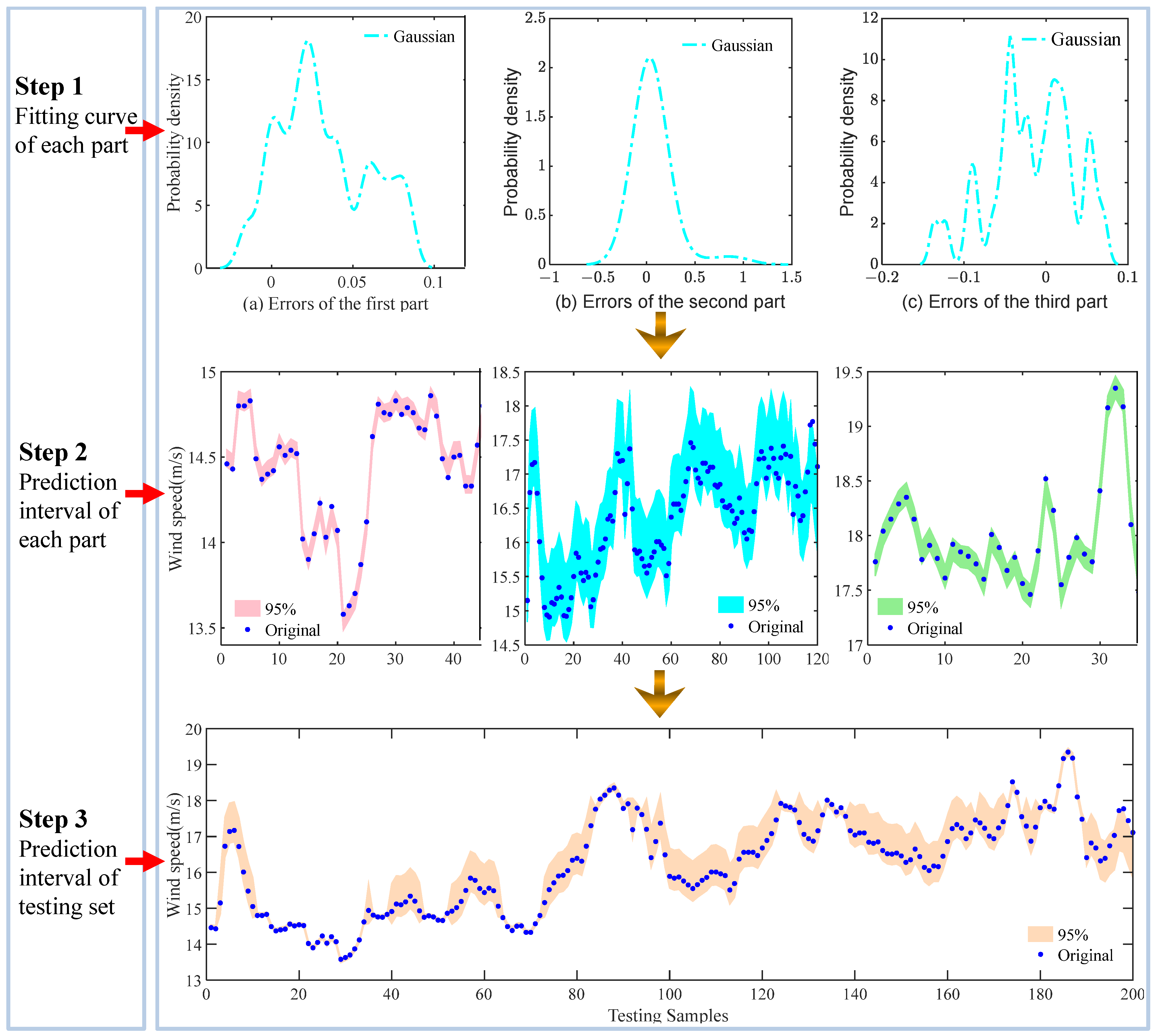
2.6. Improved Kernel Density Estimation

KDE is a statistical nonparametric estimation method. This method can simulate the probability distribution curve of predicted wind speed without assuming the prior distribution of data. Therefore, KDE is a very effective probabilistic prediction research method. In this study, wind speed point forecasting error is used as the input of KDE. The forecasting error $e$ indicates the deviation between the actual wind speed and the predicted wind speed, and then the PDF of the error $e$ can be expressed as:

$$f(e)=\frac{1}{nh}{\displaystyle \sum _{i=1}^{n}K\left(\frac{e-e_i}{h}\right)}$$

(29)

in which $n$ means the sample size; $h$ denotes bandwidth; $K(\cdot )$ indicates kernel function; $e_i$ expresses the error sample.

It can be seen from Formula (29) that kernel function and bandwidth are two important parameters that affect the accuracy of KDE. Numerous studies [43] have shown that different kernel functions have little impact on the final results. Considering the good continuity and smoothness of Gaussian functions, this paper chooses the Gaussian function as the kernel function of KDE, and its expression is as follows:

$$K(x)=\frac{1}{\sqrt{2\pi }}\exp \left(-\frac{1}{2}{x}^2\right)$$

(30)

Compared with the kernel function, the bandwidth has a greater impact on the accuracy of KDE, so it is particularly important to find the optimal bandwidth. In this paper, the proposed IWHO is used to optimize the bandwidth and form an improved kernel density estimation (IKDE). The objective function of the optimization process is as follows:

$$\begin{array}{l}fitness(\cdot )=\min CWC=PINAW\left(1+\gamma e^{-\eta \left(PICP-\left(1-\alpha \right)\right)}\right)\\ \gamma =\left\{\begin{array}{c}0,PICP\ge 1-\alpha \\ 1,PICP<1-\alpha \end{array}\right.\end{array}$$

(31)

where $PINAW$ and $PICP$ represent the PI normalized averaged width and PI coverage probability, respectively. $\gamma$ and $\eta$ are parameters that determine the degree of punishment. In this study, $\gamma =2,\eta =1$; $1-\alpha$ is the confidence level.

The PDF $f(e)$ of forecasting error $e$ is calculated through KDE and curve fitting. Then, $f(e)$ is integrated according to Equation (32) to obtain an estimate interval $\left[{\Delta }_l,{\Delta }_u\right]$ of error $e$ at $1-\alpha$ confidence level, satisfying the condition $P\left({\Delta }_l<e<{\Delta }_u\right)=1-\alpha$. Thus, at a given confidence level $1-\alpha$, the confidence interval for the prediction results of the wind speed is $\left[\widehat{y}+{\Delta }_l,\widehat{y}+{\Delta }_u\right]$.

$$\left\{\begin{array}{l}{\displaystyle {\int }_{-\infty }^{{\Delta }_l}\frac{1}{\sqrt{2\pi }nh}{\displaystyle \sum _{i=1}^n\exp \left(-\frac{1}{2}{\left(\frac{e-e_i}{h}\right)}^2\right)}de}=\alpha /2\hfill \\ {\displaystyle {\int }_{-\infty }^{{\Delta }_u}\frac{1}{\sqrt{2\pi }nh}{\displaystyle \sum _{i=1}^n\exp \left(-\frac{1}{2}{\left(\frac{e-e_i}{h}\right)}^2\right)}de}=1-\alpha /2\hfill \end{array}\right.$$

(32)

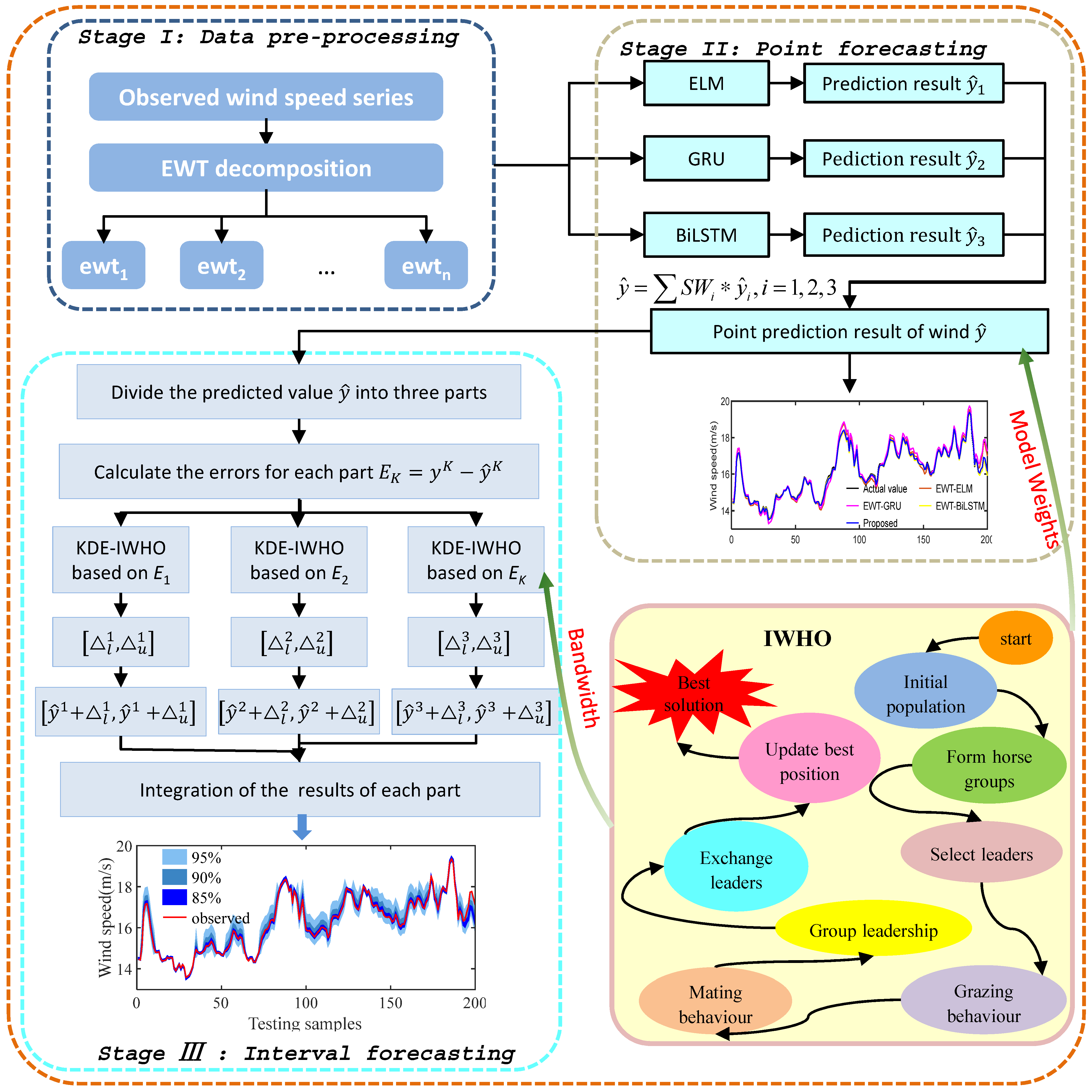
2.7. The Structure and Process of the Proposed Model

In order to provide richer information for the power system, a new point-interval wind speed prediction model EWT-EGB-IWHO IKDE based on data preprocessing, ensemble learning, and the swarm intelligence optimization algorithm is constructed in this paper. Considering the diversity and low correlation of the basic predictors [25], this paper chooses ELM, GRU, and BiLSTM as the basic predictors. IKDE is used to post-process the wind speed point forecasting values to obtain the interval forecasting results of wind speed. The structure and process of the proposed method are illustrated in Figure 1. The specific implementation process is summarized briefly below:

Stage 1: Data preprocessing. The observed wind speed $y_t=[y_1,y_2,\cdots ,y_n]$ is decomposed into several subsequences by EWT to increase the wind speed forecasting precision.

Stage 2: Point prediction. For each wind speed subcomponent, the input and output of the prediction model are designed according to the input–output structure in Figure 1. Then, three submodels, ELM, GRU, and BiLSTM, are used for point prediction, respectively, and the corresponding point prediction results ${\widehat{y}}_j=[{\widehat{y}}_{j1},{\widehat{y}}_{j2},\cdots ,{\widehat{y}}_{jn}],j=1,2,3$ are obtained. Then, the forecasting values of the three sub-models are weighted to obtain the final wind speed point prediction results, which were marked as $\widehat{y}={\displaystyle {\sum }_{j=1}^{3}S{W}_j\ast }{\widehat{y}}_j$. During this process, the weights $[S{W}_1,S{W}_2,S{W}_3]$ of the three submodels are optimized using IWHO. The fitness function is defined as follows:

$$fitness(\cdot )=\min MAE=\frac{1}{n}{\displaystyle {\sum }_{t=1}^n\left|y_t-{\widehat{y}}_t\right|}$$

(33)

Stage 3: Interval prediction. Firstly, the predicted wind speed is divided into three parts according to their mean and standard variance. The prediction wind speed of part $k$ is denoted as ${\widehat{y}}^k=[{\widehat{y}}_1^k,{\widehat{y}}_2^k,\cdots ,{\widehat{y}}_{nk}^k]$, where $nk$ is the number of the data in part $k$. Secondly, the corresponding errors of the three parts are labeled $E^k=[e_1^k,e_2^k,\cdots ,e_{nk}^k]$. IKDE is utilized to calculate the PDF of $E^k$, and then the PI $[{\Delta }_l^k,{\Delta }_u^k]$ of $E^k$ can be obtained through the inverse operation of the cumulative distribution of this PDF. Thus, the PI of the corresponding wind speed is $[{\widehat{y}}^k+{\Delta }_l^k,{\widehat{y}}^k+{\Delta }_u^k]$. Finally, the interval prediction results of the testing set are acquired by combining the interval prediction results of the three parts.

3. Case Study

To test the point and interval forecasting capabilities of the developed system, three sets of experiments were carried out on three datasets collected from a Los Angeles wind farm in 2012. All experiments in this study were run on the same platform: MATLAB R2020b on Windows 10 with a 1.6 GHz Intel Core i5-8250U CPU. All models in point prediction have six input nodes and one output node.

Table 1. Relevant parameters of the proposed model.

Model	Parameter	Value
ELM	Number of hidden neurons	6
	Transfer function	sig
GRU	Number of hidden neurons	30
	Max epochs	50
	Initial learning rate	0.01
BiLSTM	Number of hidden neurons	30
	Max epochs	50
	Initial learning rate	0.01
IWHO-EGB	$N$ Population size	20
	$ite{r}_{Max}$ Maximum iterations	50
	$PS$ Stallions percentage	0.2
	$ub$ Upper limit of weight	1
	$lb$ Lower limit of weight	0
IKDE	$N$ Population size	10
	$ite{r}_{Max}$ Maximum iterations	20
	$PS$ Stallions percentage	0.2
	$ub$ Upper limit of weight	0.1
	$lb$ Lower limit of weight	0.005

shows the parameters of the EWT-EGB-IWHO-IKDE model.

3.1. Data Description

To assess the performance of the presented model, three sets of open data (shown in Figure 2) from America’s national renewable energy laboratory (https://maps.nrel.gov/wind-prospector/ accessed on 18 October 2023) were selected as experimental samples. Taking into account the effects of different climate characteristics, three datasets were collected from three different sites and different seasons in the Los Angeles area in 2012. All three datasets have a 5 min sampling frequency, which is processed as 15 min data in this paper. Each dataset contains 1000 samples, of which 1–700 data points are the training set, 701–800 data points are the validation set, and the remaining samples are the testing set.

Table 2. Statistical characteristics of the three datasets.

Dataset	Sample	Mean (m/s)	Median (m/s)	Max (m/s)	Min (m/s)	Std. (m/s)
Site1	Training	12.3907	12.6000	27.9600	0.4100	5.4978
	Testing	16.2023	16.3800	19.3500	13.5800	1.3068
	Validation	5.2517	2.8350	15.1600	0.3100	5.1152
	All samples	12.4391	13.4050	27.9600	0.3100	5.6648
Site2	Training	11.3606	11.3550	25.8300	0.3600	3.9136
	Testing	6.7988	5.3450	17.3000	0.4200	5.1558
	Validation	16.9875	17.3700	21.9900	12.8700	2.6959
	All samples	11.0109	11.5350	25.8300	0.3600	4.8934
Site3	Training	5.0691	4.5600	14.8300	0.0900	3.6591
	Testing	8.9383	8.0300	16.4400	3.3200	3.1747
	Validation	4.2931	4.2750	7.6200	0.4200	1.5805
	All samples	5.7654	5.5300	16.4400	0.0900	3.7677

lists the statistics for the three datasets.

As shown in Figure 2, the trends and fluctuations of the three datasets are completely different. This can test the validity of the presented model on different feature data. Table 2 shows that the standard deviations of the three datasets are 5.6648 m/s, 4.8934 m/s, and 3.7677 m/s, respectively, indicating significant volatility and instability in all three wind speed sequences. This is also the primary reason for data preprocessing in this paper.

3.2. Evaluation Indicators

3.2.1. Point Prediction

The mean absolute error (MAE), root mean square error (RMSE), mean absolute percentage error (MAPE), and coefficient of determination (R²) commonly used in regression prediction are chosen as the evaluation criteria for point prediction models. MAE can avoid mutual cancellation of positive and negative errors; RMSE, also known as standard error, is used to reflect the degree of discretization of data; MAPE reflects the ratio of prediction error to observed values; and R² is used to describe the goodness of fit between predicted and observed wind speeds. The definitions of these evaluation indicators are given in

Table 3. Definition of evaluation indicators.

Metric	Description	Equation
MAE	Mean absolute error	Refer to Equation (33)
RMSE	Root mean square error	$RMSE=\sqrt{\frac{1}{n}{\displaystyle {\sum }_{t=1}^n{\left(y_t-{\widehat{y}}_t\right)}^2}}$
MAPE	Mean absolute percentage error	$MAPE=\frac{1}{n}{\displaystyle {\sum }_{t=1}^n\left|\frac{y_t-{\widehat{y}}_t}{y_t}\right|}\times 100\%$
R2	Coefficient of determination	$R^2=1-\frac{{\displaystyle {\sum }_{t=1}^n{(y_t-{\widehat{y}}_t)}^2}}{{\displaystyle {\sum }_{t=1}^n{(y_t-\overline{y})}^2}}$
PICP	PI coverage probability	$PICP=\frac{1}{n}{\displaystyle {\sum }_{t=1}^n{\xi }_t},{\xi }_t=\left\{\begin{array}{l}1,y_t\in \left[{\widehat{y}}_t^L,{\widehat{y}}_t^U\right]\hfill \\ 0,otherwise\hfill \end{array}\right.$
PINAW	PI normalized average width	$PINAW=\frac{1}{n\left(Ma{x}_y-Mi{n}_y\right)}{\displaystyle {\sum }_{t=1}^n\left({\widehat{y}}_t^U-{\widehat{y}}_t^L\right)}$
AIS	Average interval score	$\begin{array}{l}AIS=\frac{1}{n}{\displaystyle {\sum }_{t=1}^n{\phi }_t},\\ {\phi }_t=\left\{\begin{array}{l}-2\alpha {\zeta }_t-4\left({\widehat{y}}_t^L-y_t\right),y_t<{\widehat{y}}_t^L\hfill \\ -2\alpha {\zeta }_t,y_t\in \left[{\widehat{y}}_t^L,{\widehat{y}}_t^U\right]\hfill \\ -2\alpha {\zeta }_t-4\left(y_t-{\widehat{y}}_t^U\right),y_t>{\widehat{y}}_t^U\hfill \end{array}\right.\\ {\zeta }_t={\widehat{y}}_t^U-{\widehat{y}}_t^L\end{array}$

Note: ${\widehat{y}}_t$ and $y_t$ represent the $t$-th forecasting and observed wind speeds, respectively; $\overline{y}$ means the average observed value; ${\widehat{y}}_t^U$ and ${\widehat{y}}_t^L$ denote the upper and lower limits of the $t$-th sample PI, respectively; $Ma{x}_y$ and $Mi{n}_y$ stand for the maximum and minimum observed values, respectively; $n$ indicates the testing set size.

.

3.2.2. Interval Prediction

PICP and PINAW are commonly used to evaluate the effectiveness of interval forecasting. However, it does not follow that the larger the PICP or the smaller the PINAW, the more reliable the interval forecasting results. PICP and PINAW are two indicators with opposing properties, and sometimes the increase in PICP comes at the cost of increasing PINAW. This is not conducive to the comprehensive measurement of interval prediction. Therefore, this paper introduces an evaluation tool called average interval score (AIS), which can comprehensively consider both coverage and interval width, making it more suitable for assessing the comprehensive ability of the model’s interval forecasting. All evaluation indicators are defined in Table 3.

3.3. Experimental Analysis

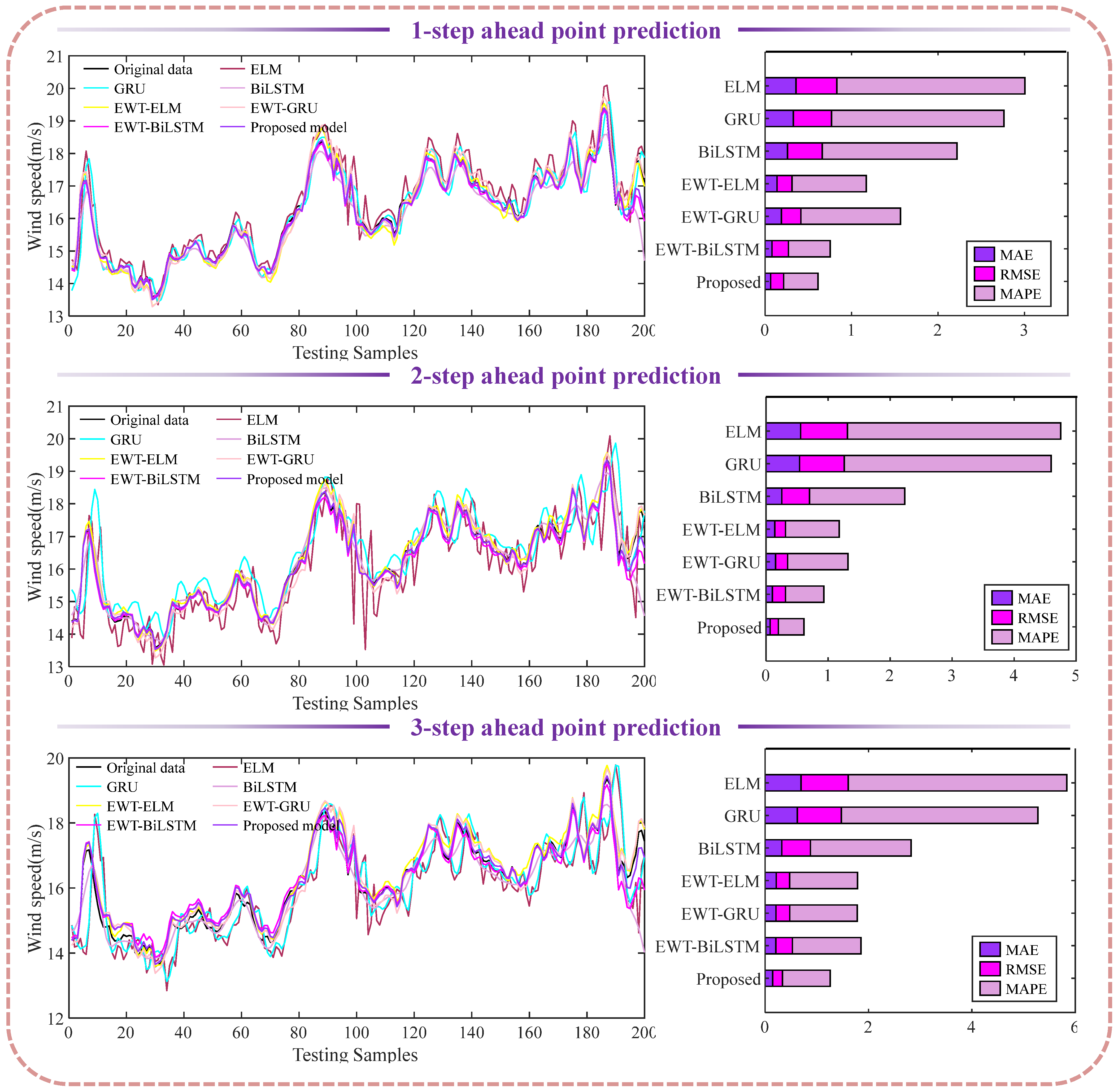
3.3.1. Experiment I: Comparison with Each Module

In this experiment, the developed model is compared with the modules (including ELM, GRU, BiLSTM, EWT-ELM, EWT-GRU, EWT-BiLSTM model) to prove the validity of each module in the integrated model.

Table 4. Comparison of prediction errors of different models in Experiment I.

	1-Step				2-Step				3-Step
	MAE (m/s)	RMSE (m/s)	MAPE (%)	R2	MAE (m/s)	RMSE (m/s)	MAPE (%)	R2	MAE (m/s)	RMSE (m/s)	MAPE (%)	R2
Site1
ELM	0.3570	0.4728	2.1736	0.8675	0.5594	0.7548	3.4388	0.6647	0.6952	0.9119	4.2301	0.5107
GRU	0.3277	0.4409	1.9935	0.8848	0.5411	0.7211	3.3338	0.6940	0.6240	0.8496	3.8049	0.5752
BiLSTM	0.2598	0.4006	1.5575	0.9049	0.2544	0.4483	1.5357	0.8818	0.3237	0.5540	1.9469	0.8194
EWT-ELM	0.1377	0.1739	0.8589	0.9821	0.1417	0.1730	0.8637	0.9824	0.2154	0.2587	1.3119	0.9606
EWT-GRU	0.1897	0.2246	1.1513	0.9701	0.1551	0.1954	0.9699	0.9775	0.2119	0.2665	1.3048	0.9582
EWT-BiLSTM	0.0808	0.1898	0.4806	0.9787	0.1038	0.2119	0.6162	0.9736	0.2093	0.3200	1.3239	0.9397
Proposed model	0.0645	0.1501	0.3978	0.9866	0.0669	0.1335	0.4121	0.9895	0.1474	0.1891	0.9226	0.9790
Site2
ELM	0.6359	0.7720	30.0916	0.9775	0.6661	0.7979	29.2131	0.9759	0.7201	0.9153	29.1313	0.9683
GRU	0.6616	0.7626	29.3708	0.9780	0.6530	0.8087	26.6273	0.9753	0.6325	0.8708	16.3146	0.9713
BiLSTM	0.4495	0.5229	19.5257	0.9897	0.5142	0.6002	23.0972	0.9864	0.3426	0.4097	11.8257	0.9937
EWT-ELM	0.3888	0.4969	14.4731	0.9907	0.2000	0.2532	7.6905	0.9976	0.2884	0.3569	10.2520	0.9952
EWT-GRU	0.1362	0.1676	4.3028	0.9989	0.4014	0.5202	11.7996	0.9898	0.5507	0.6689	22.9484	0.9831
EWT-BiLSTM	0.1580	0.1912	6.6465	0.9986	0.1767	0.2120	8.0111	0.9983	0.2862	0.3516	7.9880	0.9953
Proposed model	0.0960	0.1198	2.8844	0.9995	0.1218	0.1609	3.8680	0.9990	0.1794	0.2370	4.8923	0.9979
Site3
ELM	0.3833	0.6166	4.5139	0.9621	0.6948	1.0138	8.4530	0.8975	1.0543	1.4322	12.6841	0.7955
GRU	0.3698	0.5745	4.5143	0.9671	0.7781	1.0963	9.6551	0.8802	1.2204	1.5846	14.8457	0.7496
BiLSTM	0.5200	0.6508	5.4658	0.9578	0.3108	0.4327	3.7440	0.9813	0.3026	0.4384	3.6605	0.9808
EWT-ELM	0.0898	0.1132	1.1306	0.9987	0.2417	0.3148	2.8992	0.9901	0.2550	0.3148	2.9582	0.9901
EWT-GRU	0.2829	0.3898	2.9384	0.9849	0.3227	0.4222	3.6803	0.9822	0.5071	0.6636	5.7460	0.9561
EWT-BiLSTM	0.2839	0.2441	1.8321	0.9941	0.1434	0.1818	1.7636	0.9967	0.1538	0.2368	1.4846	0.9944
Proposed model	0.0824	0.1096	0.9897	0.9988	0.1323	0.1598	1.7568	0.9975	0.1200	0.1996	1.2008	0.9960

compares the point forecasting results of all comparative models at three sites, with blod font indicating the optimal results. Figure 3 illustrates the multi-step forecasting results of all methods using site1 as an example. Based on Table 4 and Figure 3, the specific analysis is as follows:

(1) For site1, the presented model based on all evaluation indicators outperforms the benchmark models in multi-step ahead prediction. The stack visualization of MAE, RMSE, and MAPE in Figure 3 illustrates this even more clearly. The R² values of the development model in multi-step ahead prediction are 0.9866, 0.9895, and 0.9790, respectively, which reflect its excellent fitting performance. The experimental results prove the significant contribution of EWT in wind speed prediction. Taking 1-step as an example, the MAPEs of ELM and EWT-ELM, GRU and EWT-GUR, and BiLSTM and EWT-BiLSTMS are 2.1736% and 0.1377%, 1.9935% and 1.1513%, and 1.5575% and 0.4806%, respectively. In addition, as the forecasting steps increase, the prediction accuracy of almost all models decreases by varying degrees. For example, the MAPEs of the proposed model in the three prediction steps are 0.3978% (1-step), 0.4121% (2-step), and 0.9226% (3-step), respectively.

(2) For site2, interestingly, as the prediction time scale increases, the prediction accuracy of the GRU, BiLSTM, and EWT-ELM models improves, while the prediction accuracy of the BiLSTM, EWT-GRU, and EWT-BiLSTM models decreases. This indicates that each model performs differently for the datasets with different features, which is also an important reason for this article’s proposal to integrate multiple predictors. The developed model has greater advantages in predicting performance than the comparative models. Taking 3-step ahead prediction for instance, the MAPEs of the presented method and the six comparison models are 4.8923%, 29.1313%, 16.3146%, 11.8257%, 10.2520%, 2.9484%, and 7.9880%, respectively.

(3) For site3, the proposed model demonstrates the best predictive ability in all prediction steps based on all evaluation indicators, with MAPEs of 0.9897%, 1.7568%, and 1.2008% for the three prediction steps, respectively. Its R² values in the three prediction steps are 0.9988, 0.9975, and 0.9960 respectively, showing excellent fitting ability. Among the three single prediction models, ELM and GRU perform similarly, while BiLSTM has lower accuracy than ELM and GRU in 1-step prediction, but higher accuracy than ELM and GRU in 2-step and 3-step prediction. It is clear that the forecasting ability of a model is not stable in the face of different datasets.

3.3.2. Experiment II: Comparison with Models Based on Different Decomposition Algorithms

This experiment aims to compare the contributions of several commonly used data decomposition algorithms for wind speed prediction. Three integrated models EMD-EGB-IWHO (EMD-based), VMD-EGB-IWHO (VMD-based), and CEEMD-EGB-IWHO (CEEMD-based) were selected to compare with the proposed model. In other words, the basic predictor and intelligent optimization algorithm in these three integrated models are the same as those in the proposed models, except for different data preprocessing techniques.

Table 5. Comparison of prediction errors of different models in experiment II.

	1-Step				2-Step				3-Step
	MAE (m/s)	RMSE (m/s)	MAPE (%)	R2	MAE (m/s)	RMSE (m/s)	MAPE (%)	R2	MAE (m/s)	RMSE (m/s)	MAPE (%)	R2
Site1
EMD-based	0.1376	0.2517	0.8450	0.9627	0.2463	0.3765	1.5227	0.9166	0.2654	0.3748	1.6411	0.9173
CEEMD-based	0.0752	0.1458	0.4851	0.9855	0.0900	0.1429	0.5601	0.9880	0.1426	0.2216	0.8894	0.9711
VMD-based	0.1190	0.1639	0.7284	0.9842	0.1292	0.1791	0.7885	0.9811	0.1768	0.2363	1.0805	0.9671
Proposed model	0.0645	0.1501	0.3978	0.9866	0.0669	0.1335	0.4121	0.9895	0.1474	0.1891	0.9226	0.9790
Site2
EMD-based	0.2626	0.3267	9.6082	0.9960	0.2286	0.3118	5.6527	0.9963	0.2909	0.3956	8.1681	0.9941
CEEMD-based	0.1061	0.1475	2.9597	0.9992	0.1529	0.2099	3.9996	0.9983	0.2606	0.3254	9.2805	0.9960
VMD-based	0.2896	0.4151	9.0222	0.9935	0.4857	0.6518	12.642	0.9839	0.2530	0.3318	7.5103	0.9958
Proposed model	0.0960	0.1198	2.8844	0.9995	0.1218	0.1609	3.8680	0.9990	0.1794	0.2370	4.8923	0.9979
Site3
EMD-based	0.1072	0.1792	1.3822	0.9968	0.3377	0.4327	4.0238	0.9813	0.2040	0.3133	2.4345	0.9902
CEEMD-based	0.1536	0.2443	1.9178	0.9940	0.1709	0.2545	2.1584	0.9935	0.1954	0.2959	2.4724	0.9913
VMD-based	0.1740	0.2662	2.0130	0.9929	0.2157	0.3095	2.5698	0.9904	0.2657	0.3730	3.0462	0.9861
Proposed model	0.0824	0.1096	0.9897	0.9988	0.1323	0.1598	1.7568	0.9975	0.1200	0.1996	1.2008	0.9960

shows the results of multi-step prediction for different models in the three datasets, where the best results are shown in bold.

The following conclusions emerge from Table 5:

(1) For site1, the proposed model achieves the best predictive performance in almost all evaluation indicators. Although RMSE in 1-step ahead forecasting and MAE and MAPE in 3-step ahead forecasting show that the CEEMD-based model is slightly better than the proposed method, the proposed model has more advantages overall. The presented model acquires the best R² in all prediction steps, indicating that it has the best fitting ability. Among the three data preprocessing methods, CEEMD is better than VMD, and EMD is the worst. Taking 3-step prediction for instance, the MAPEs of the models based on these three methods are 0.8894%, 1.0805%, and 1.6411%, respectively.

(2) For site2, the presented model outperforms the comparison models in terms of MAE, RMSE, MAPE, and R². Figure 4 also clearly demonstrates this conclusion. The CEEMD-based model performs better in 1-step and 2-step predictions than the EMD- and VMD-based models, but performs slightly worse in 3-step predictions. It has a common feature with the proposed model that as the forecasting steps increase, the forecasting precision decreases. However, the models based on EMD and VMD do not follow this rule. In other words, compared to the 1-step prediction accuracy, the EMD-based model improves the forecasting precision in 2-step prediction, while the VMD-based model actually decreases the prediction accuracy. Moreover, in terms of prediction accuracy, EMD-based models are better than VMD-based models in 1-step prediction but worse than VMD-based models in 3-step prediction. It is further confirmed that EWT is more robust than EMD, VMD, and CEEMD. This is because the EWT algorithm has good frequency local characteristics and can accurately extract the frequency information of the signal.

(3) For site3, according to all evaluation indexes, the prediction performance of the presented system is the best and the most stable in each forecasting step. However, the predictive abilities of the comparison models based on EMD, CEEMD, and VMD are not stable in the three prediction steps. For example, their MAPEs for 1-step prediction are 1.3822%, 1.9178%, and 2.0130%, respectively. The EMD-based model performs the best, while the MAPEs for 2-step prediction are 4.0238%, 2.1584%, and 2.5698%, respectively. The EMD-based model performs the worst.

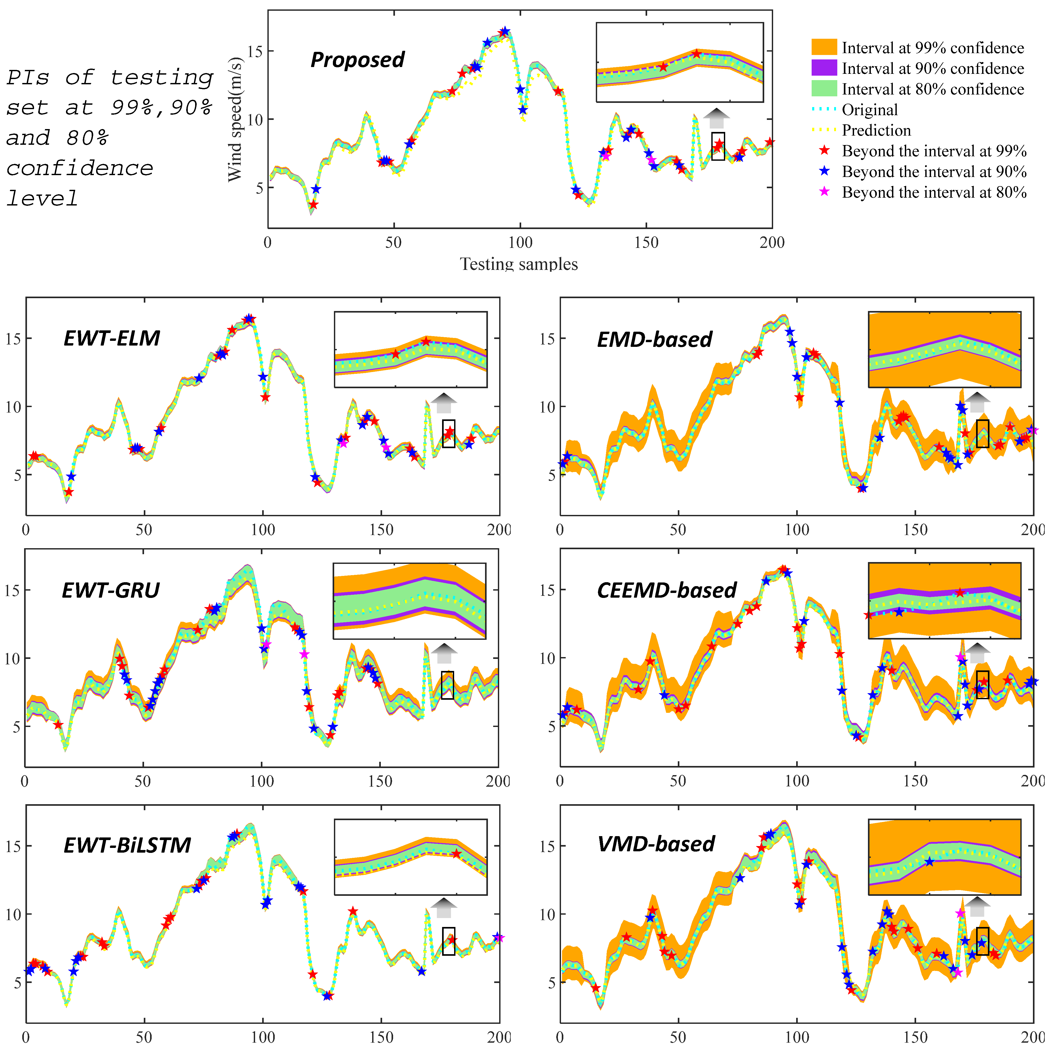
3.3.3. Experiment III: Comparison of Interval Estimates for All Models

Point prediction is deterministic, and the information it provides has great limitations. In fact, large-scale wind power grid-connected systems require richer uncertainty information to specify scheduling plans. Therefore, a PI estimation method of wind speed using IKDE is proposed. Using the point forecasting error of wind speed as the input of IKDE, the wind speed PIs at each confidence level are estimated to assess the uncertainty of wind speed. To be fair, the point forecasting results of all models are post-processed in the same way. By analyzing the uncertainty, the performance of the presented model in interval prediction is verified.

Considering the significant fluctuations in forecasting errors corresponding to different predicted wind speeds, the predicted wind speeds are separated into different parts. The prediction error for each part is then estimated using IKDE. Some studies have shown that partitioning strategies based on mean and standard deviation can achieve better PIs compared with average partitioning strategies [44,45]. The specific operation is as follows:

$${\widehat{y}}^1<\mu -\sigma ,\mu -\sigma \le {\widehat{y}}^2\le \mu +\sigma ,{\widehat{y}}^3>\mu +\sigma$$

(34)

where $\mu$ and $\sigma$ stand for the mean and standard deviation of the predicted wind speed, respectively; ${\widehat{y}}^1$, ${\widehat{y}}^2$, and ${\widehat{y}}^3$ indicate the three parts. Then, the corresponding error $E^k=[e_1^k,e_2^k,\cdots ,e_{nk}^k],k=1,2,3$ of each part is calculated. At a given confidence level, the confidence interval $[{\Delta }_l^k,{\Delta }_u^k]$ of each error part is estimated by the IKDE, where ${\Delta }_l^k$ and ${\Delta }_u^k$ stand for the lower and upper bounds of the probability estimation for the $k$-th error part, respectively. By summing the point prediction results with the error confidence interval, the wind speed PIs for each part are $[{\widehat{y}}^k+{\Delta }_l^k,{\widehat{y}}^k+{\Delta }_u^k]$. Finally, the predicted intervals of wind speed for the three parts are recombined into the PI of the testing set. Taking the interval estimation of 1-step ahead prediction at 95% confidence level for site1 as an example, the calculation process is illustrated in Figure 5. As shown in step 1 of Figure 5, the errors in these three parts have completely different distributions. The interval prediction results can, therefore, be more accurate only when each part error is estimated separately.

In this experiment, the PIs of EWT-ELM, EWT-GRU, EWT-BiLSTM, EMD-based, CEEMD-based, VMD-based, and the proposed model EWT-EGB-IWHO were calculated using the same partitioning strategy and the same probability estimation method, respectively.

Table 6. Comparison of interval predictions between the proposed and comparison models at 99% confidence level.

$\mathit{\alpha }=0.01$		1-Step			2-Step			3-Step
		PICP	PINAW	AIS	PICP	PINAW	AIS	PICP	PINAW	AIS
Site1	EWT-ELM	0.9950	0.3894	−0.0459	0.9900	0.1849	−0.0198	0.9900	0.1294	−0.0157
	EWT-GRU	0.9950	0.3760	−0.0445	0.9950	0.1383	−0.0160	0.9950	0.1824	−0.0211
	EWT-BiLSTM	0.9900	0.4094	−0.0473	0.9950	0.1483	−0.0172	1.0000	0.2337	−0.0270
	EMD-based	0.9950	0.3065	−0.0362	0.9950	0.3273	−0.0380	0.9900	0.3486	−0.0410
	CEEMD-based	0.9950	0.2132	−0.0255	0.9900	0.1493	−0.0174	0.9950	0.2352	−0.0275
	VMD-based	0.9900	0.1856	−0.0218	0.9900	0.1935	−0.0228	0.9900	0.2299	−0.0273
	Proposed model	0.9950	0.1940	−0.0161	0.9900	0.0913	−0.0109	0.9950	0.1097	−0.0120
Site2	EWT-ELM	0.9900	0.1063	−0.0360	0.9950	0.0551	−0.0186	0.9900	0.0847	−0.0287
	EWT-GRU	1.0000	0.0361	−0.0122	0.9900	0.1195	−0.0404	0.9900	0.1566	−0.0533
	EWT-BiLSTM	0.9900	0.0365	−0.0124	0.9950	0.0462	−0.0162	0.9900	0.0743	−0.0184
	EMD-based	0.9950	0.1147	−0.0397	0.9950	0.1147	−0.0394	0.9950	0.1304	−0.0449
	CEEMD-based	0.9900	0.0540	−0.0186	0.9950	0.0716	−0.0242	0.9900	0.0771	−0.0266
	VMD-based	0.9950	0.0792	−0.0268	0.9950	0.0974	−0.0329	0.9900	0.0746	−0.0254
	Proposed model	0.9900	0.0254	−0.0087	0.9900	0.0338	−0.0118	0.9950	0.0570	−0.0174
Site3	EWT-ELM	0.9900	0.0396	−0.0107	0.9900	0.0847	−0.0287	0.9900	0.0902	−0.0239
	EWT-GRU	0.9900	0.0986	−0.0259	0.9900	0.1566	−0.0533	0.9900	0.1540	−0.0406
	EWT-BiLSTM	0.9950	0.0359	−0.0096	0.9900	0.0543	−0.0194	0.9950	0.0618	−0.0163
	EMD-based	0.9950	0.1326	−0.0374	0.9950	0.1304	−0.0449	0.9900	0.1957	−0.0565
	CEEMD-based	0.9950	0.1423	−0.0391	0.9900	0.1304	−0.0266	0.9900	0.1637	−0.0456
	VMD-based	0.9900	0.1456	−0.0415	0.9900	0.0746	−0.0254	0.9950	0.1630	−0.0455
	Proposed model	0.9900	0.0322	−0.0087	0.9950	0.0570	−0.0144	0.9900	0.0513	−0.0135

,

Table 7. Comparison of interval predictions between the proposed and comparison models at 90% confidence level.

$\mathit{\alpha }=0.1$		1-Step			2-Step			3-Step
		PICP	PINAW	AIS	PICP	PINAW	AIS	PICP	PINAW	AIS
Site1	EWT-ELM	0.9000	0.1729	−0.2908	0.9100	0.0696	−0.0906	0.9000	0.0943	−0.1334
	EWT-GRU	0.9050	0.1794	−0.2824	0.8950	0.0986	−0.1334	0.9000	0.1342	−0.1802
	EWT-BiLSTM	0.9000	0.1845	−0.3150	0.9100	0.0768	−0.1386	0.9050	0.1605	−0.2390
	EMD-based	0.9100	0.1936	−0.2078	0.8950	0.1711	−0.2792	0.9000	0.2014	−0.3083
	CEEMD-based	0.9050	0.1562	−0.2138	0.8950	0.0699	−0.1307	0.9000	0.1005	−0.1980
	VMD-based	0.8950	0.1881	−0.1907	0.9050	0.0930	−0.1583	0.9000	0.1271	−0.1972
	Proposed model	0.9050	0.0836	−0.1826	0.9000	0.0607	−0.0826	0.9000	0.0842	−0.1118
Site2	EWT-ELM	0.8950	0.0794	−0.3247	0.9000	0.0457	−0.1713	0.9050	0.0552	−0.2417
	EWT-GRU	0.8950	0.0294	−0.1118	0.9000	0.0786	−0.3350	0.9000	0.1063	−0.4491
	EWT-BiLSTM	0.8950	0.0270	−0.1084	0.9050	0.0266	−0.1060	0.9000	0.0439	−0.1696
	EMD-based	0.9050	0.0521	−0.2482	0.8950	0.0591	−0.2652	0.9100	0.0687	−0.3251
	CEEMD-based	0.9000	0.0269	−0.1281	0.8950	0.0356	−0.1711	0.9050	0.0435	−0.1919
	VMD-based	0.9100	0.0554	−0.2273	0.9050	0.0805	−0.3056	0.9000	0.0397	−0.2063
	Proposed model	0.9050	0.0190	−0.0753	0.9100	0.0426	−0.1950	0.9050	0.0454	−0.1517
Site3	EWT-ELM	0.9050	0.0280	−0.0865	0.9050	0.0552	−0.2417	0.9000	0.0692	−0.2110
	EWT-GRU	0.8950	0.0674	−0.2156	0.9000	0.1063	−0.4491	0.9000	0.1032	−0.3549
	EWT-BiLSTM	0.9100	0.0244	−0.0800	0.9000	0.0554	−0.2117	0.9050	0.0404	−0.1302
	EMD-based	0.9050	0.0318	−0.1570	0.9100	0.0687	−0.3251	0.8950	0.0490	−0.2421
	CEEMD-based	0.9050	0.0420	−0.2078	0.9050	0.0435	−0.1919	0.9100	0.0530	−0.2524
	VMD-based	0.9000	0.0429	−0.2032	0.9000	0.0512	−0.2063	0.8950	0.0605	−0.2279
	Proposed model	0.9000	0.0232	−0.0713	0.9050	0.0439	−0.1696	0.9100	0.0314	−0.1087

, and

Table 8. Comparison of interval predictions between the proposed and comparison models at 80% confidence level.

$\mathit{\alpha }=0.2$		1-Step			2-Step			3-Step
		PICP	PINAW	AIS	PICP	PINAW	AIS	PICP	PINAW	AIS
Site1	EWT-ELM	0.8000	0.1286	−0.4599	0.8000	0.0556	−0.1635	0.7900	0.0698	−0.2016
	EWT-GRU	0.8100	0.1257	−0.4578	0.8000	0.0781	−0.2345	0.8100	0.1004	−0.3159
	EWT-BiLSTM	0.8000	0.1341	−0.4958	0.8050	0.0297	−0.1954	0.7950	0.0673	−0.3624
	EMD-based	0.8000	0.0641	−0.2835	0.8050	0.1105	−0.4411	0.8000	0.1305	−0.4884
	CEEMD-based	0.8100	0.0290	−0.1550	0.7950	0.0469	−0.1983	0.8050	0.0691	−0.2930
	VMD-based	0.8050	0.0577	−0.2318	0.7950	0.0662	−0.2479	0.8000	0.0965	−0.2930
	Proposed model	0.8000	0.1282	−0.4787	0.8150	0.0482	−0.1453	0.8050	0.0652	−0.1943
Site2	EWT-ELM	0.7900	0.0584	−0.5555	0.7900	0.0370	−0.3145	0.7950	0.0442	−0.4104
	EWT-GRU	0.8100	0.0218	−0.1983	0.8050	0.0606	−0.5657	0.8050	0.0826	−0.7676
	EWT-BiLSTM	0.8100	0.0227	−0.1920	0.7950	0.0298	−0.2949	0.8050	0.0340	−0.3023
	EMD-based	0.7950	0.0458	−0.4132	0.7950	0.0413	−0.4310	0.8050	0.0483	−0.5162
	CEEMD-based	0.8000	0.0186	−0.2046	0.7950	0.0271	−0.2766	0.7950	0.0357	−0.3248
	VMD-based	0.7950	0.0468	−0.3974	0.7950	0.0715	−0.5625	0.8050	0.0397	−0.3582
	Proposed model	0.8000	0.0157	−0.1352	0.8050	0.0208	−0.2199	0.8100	0.0341	−0.3008
Site3	EWT-ELM	0.8000	0.0214	−0.1511	0.7950	0.0442	−0.4104	0.7950	0.0562	−0.3739
	EWT-GRU	0.8000	0.0548	−0.3778	0.8050	0.0826	−0.7676	0.7950	0.0841	−0.6017
	EWT-BiLSTM	0.8100	0.0202	−0.1395	0.8050	0.0441	−0.3808	0.8050	0.0334	−0.2266
	EMD-based	0.8050	0.0232	−0.2273	0.8050	0.0483	−0.5162	0.8050	0.0373	−0.3515
	CEEMD-based	0.8000	0.0262	−0.2896	0.7950	0.0357	−0.3248	0.8000	0.0386	−0.3728
	VMD-based	0.8050	0.0343	−0.3055	0.8050	0.0397	−0.3582	0.8000	0.0487	−0.3703
	Proposed model	0.8000	0.0179	−0.1247	0.8100	0.0340	−0.3023	0.8050	0.0230	−0.1798

provide the interval forecasting values of different prediction steps at 99%, 90%, and 80% confidence levels for all methods, respectively. The analysis of the multiple evaluation indicators is as follows:

(1) For site1, at 99% confidence level, the proposed model achieves the best AIS and PINAW, with a relatively high PICP. Its AISs in the multi-step forecast are −0.0161, −0.0109, and −0.0120, respectively. The interval forecasting abilities of the comparison models are unstable in different forecasting steps. For example, in 1-step early prediction, EWT-ELM, EWT-GRU, and EWT-BiLSTM have close AISs and perform poorly. However, in 2-step ahead prediction, the models EMD-based and VMD-based perform poorly. Similar conclusions are obtained at the 90% confidence level. The proposed model still achieves the best AISs, which are −0.1826, −0.0826, and −0.1118 for the three prediction steps, respectively. It is worth noting that CEEMD-based performs best in 1-step ahead prediction at the 80% confidence level, where it achieves the highest PICP (0.8100) and the smallest PINAW (0.0290). However, the comprehensive index AIS of the proposed model remains the highest in the 2-step and 3-step ahead prediction. Overall, in most experiments, the interval prediction performance of the presented method is superior to that of the comparison methods.

(2) For site2, at 99% and 80% confidence levels, the proposed model outperforms the benchmark models by a landslide, followed by EWT-BiLSTM. EWT-BiLSTM outperforms the presented model in 2-step ahead prediction at the 90% confidence level. The predictive abilities of other benchmark models remain unstable for different forecasting steps. It can be observed from Table 6, Table 7 and Table 8 that the PICP of the proposed model does not always remain optimal in all experiments, but it almost always obtains a smaller PINAW and a larger AIS. This is because the forecast error fluctuation of the presented model is relatively small, so a small interval can be found to meet the corresponding probability conditions when the error is fitted with the probability density. This indicates that the point prediction result affects the reliability of the PI to some extent.

(3) For site3, the proposed model still has the best advantages compared with all the benchmark models. In 1-step ahead prediction, the proposed model obtains the smallest PINAW (0.0322, 0.0232, 0.0179) and the largest AISs (−0.0087, −0.0713, −0.1247) at all three confidence levels. The EMD-based, CEEMD-based, and VMD-based models have larger PINAW at 99% confidence level, while EWT-GRU has larger PINAW at 90% and 80% confidence levels, as confirmed in Figure 6. The proposed model achieves the maximum AIS index at all prediction steps and confidence levels, for example, AIS results of −0.0713, −0.1696, and −0.1087 at the three prediction steps at the 90% confidence level. These analyses are sufficient to demonstrate that the presented method can achieve reliable wind speed interval prediction.

4. Discussion

4.1. Significance Test of Point Prediction

According to the analysis of the point prediction results in Section 3.3.1 and Section 3.3.2, the forecasting accuracy of the proposed method is higher than other models. However, this only means that the proposed model performs well in these samples. This situation may be caused by sampling or may be accidental. The hypothesis testing method Diebold–Mariano (DM) [25] can test whether the two models have significant differences in nature, to further validate the superiority of the proposed method.

Table 9. Results of DM test for proposed and comparison models.

	Site1			Site2			Site3
	1-Step	2-Step	3-Step	1-Step	2-Step	3-Step	1-Step	2-Step	3-Step
ELM	7.3574 *	6.5137 *	7.4031 *	11.9461 **	12.2984 *	8.6157 *	3.4739 *	8.6157 *	6.6053 *
GRU	6.0446 *	6.6629 *	6.6660 *	14.2987 *	10.0245 *	6.2358 *	3.1618 *	6.2358 *	8.9628 *
BiLSTM	4.1084 *	3.0480 *	2.9419 *	15.6143 *	14.7711 *	7.9450 *	9.7314 *	7.9450 *	4.2174 *
EWT-ELM	0.8572	1.7900 ***	5.8412 *	8.8936 *	5.9151 *	7.3056 *	0.9546	7.3056 *	6.5051 *
EWT-GRU	2.9417 *	2.7935 *	5.5774 *	6.2635 *	8.9593 *	11.4720 *	8.4334 *	11.4720 *	8.4120 *
EWT-BiLSTM	2.6336 *	3.1598 *	3.4036 *	6.9916 *	5.4954 *	7.8462 *	7.2497 *	7.8462 *	5.4131 *
EMD-based	2.4400 **	4.7320 *	4.7581 *	6.5853 *	4.3216 *	3.7923 *	1.7628 ***	7.8462 *	2.4107 **
CEEMD-based	0.0983	0.3405	0.9707	2.1819 **	2.3459 **	4.9596 *	2.8860 *	4.9596 *	2.3144 **
VMD-based	1.1217	1.9378 ***	2.7354 *	8.1072 *	9.7279 *	4.6521 *	4.1650 *	4.6521 *	5.6159 *

* Is the 1% significance level. ** Is the 5% significance level. *** Is the 10% significance level.

presents the DM test results.

Most of the DM values in Table 9 are not in the interval $\left[-Z_{0.01/2},Z_{0.01/2}\right]$, indicating a 99% probability of rejecting the original hypothesis and accepting the alternative hypothesis. The smallest DM test result of the proposed model compared to the CEEMD-based model is 0.0983 (above 0) in 1-step ahead prediction at site1. This illustrates that although the point prediction results of these two models are similar (see Table 5), the proposed model is more reliable than the CEEMD-based model. In all prediction steps at site2 and site3, all DM values are greater than $Z_{0.10/2}=1.64$, demonstrating a 90% probability of significant difference between the presented method and the benchmark models. The DM test further confirms the advantages and reliability of the presented method from a statistical perspective.

4.2. Improvement in Interval Prediction Performance

The comprehensive analysis of the interval prediction results in Section 3.3.3 shows that the presented method is superior to the comparison methods in interval forecasting. When evaluating the interval prediction ability of a model, both PINAW and PICP should be taken into account. Therefore, the improvement percentage of the comprehensive evaluation index AIS is selected to quantify the improvement in the proposed model compared to the comparison models. The improvement rate of AIS is defined as follows:

$$P_{AIS}=\frac{AI{S}_{Com}^{\mu ,s}-AI{S}_{Pro}^{\mu ,s}}{AI{S}_{Com}^{\mu ,s}}\times 100\%$$

(35)

where $AI{S}_{Com}^{\mu ,s}$ and $AI{S}_{Pro}^{\mu ,s}$ represent the AIS values of the benchmark model and the proposed model at the confidence level $\mu$ ($\mu =99\%,90\%,80\%$) in $s$-step ($s=1,2,3$) ahead prediction, respectively. The AIS improvement rate of the presented model to the benchmark models is compared in

Table 10. Improvement rate of AIS.

Improvement (%)		$\mathit{\alpha }=0.01$			$\mathit{\alpha }=0.1$			$\mathit{\alpha }=0.2$
		1-Step	2-Step	3-Step	1-Step	2-Step	3-Step	1-Step	2-Step	3-Step
Site1	EWT-ELM	64.92	44.95	23.57	37.21	8.83	16.19	−4.09	11.13	3.62
	EWT-GRU	63.82	31.88	43.13	35.34	38.08	37.96	−4.57	38.04	38.49
	EWT-BiLSTM	65.96	36.63	55.56	42.03	40.40	53.22	3.45	25.64	46.39
	EMD-based	55.52	71.32	70.73	12.13	70.42	63.74	−68.85	67.06	60.22
	CEEMD-based	36.86	37.36	56.36	14.59	36.80	43.54	−208.84	26.73	33.69
	VMD-based	26.15	52.19	56.04	4.25	47.82	43.31	−106.51	41.39	33.69
Site2	EWT-ELM	75.83	36.56	39.37	76.81	−13.84	37.24	75.66	30.08	26.71
	EWT-GRU	28.69	70.79	67.35	32.65	41.79	66.22	31.82	61.13	60.81
	EWT-BiLSTM	29.84	27.16	5.43	30.54	−83.96	10.55	29.58	25.43	0.50
	EMD-based	78.09	70.05	61.25	69.66	26.47	53.34	67.28	48.98	41.73
	CEEMD-based	53.23	51.24	34.59	41.22	−13.97	20.95	33.92	20.50	7.39
	VMD-based	67.54	64.13	31.50	66.87	36.19	26.47	65.98	60.91	16.02
Site3	EWT-ELM	18.69	49.83	43.51	17.57	29.83	48.48	17.47	26.34	51.91
	EWT-GRU	66.41	72.98	66.75	66.93	62.24	69.37	66.99	60.62	70.12
	EWT-BiLSTM	9.37	25.77	17.18	10.87	19.89	16.51	10.61	20.61	20.65
	EMD-based	76.74	67.93	76.11	54.59	47.83	55.10	45.14	41.44	48.85
	CEEMD-based	77.75	45.86	70.39	65.69	11.62	56.93	56.94	6.93	51.77
	VMD-based	79.04	43.31	70.33	64.91	17.79	52.30	59.18	15.61	51.44

.

From Table 10, it is obvious that for most benchmark models, the AIS improvement of the presented model is significant. For example, in the 1-step ahead prediction at the 99% confidence level on site1, the presented model’s AIS improvements over the six benchmark models are 64.92%, 63.82%, 65.96%, 55.52%, 36.86%, and 26.15%, respectively. It is worth mentioning that in 1-step ahead prediction at the 80% confidence level on site1 and 2-step ahead prediction at the 90% confidence level on site2, the proposed model is slightly inferior to some benchmark models. This rare occurrence may be due to sampling. In general, the interval prediction capability of the presented method is better than those of the contrasting methods.

4.3. Discussion of the IWHO Performance

The effectiveness of IWHO was validated using six classic unimodal and multimodal test functions as shown in

Table 11. Description of the benchmark functions.

Function Definition	Dim	Range	fmin
$f_1(x)={\displaystyle {\sum }_{i=1}^n{x}_i{}^2}$	30	[−100, 100]	0
$f_2(x)={\displaystyle {\sum }_{i=1}^n\left|x_i\right|+{\displaystyle \prod _{i=1}^n\left|x_i\right|}}$	30	[−10, 10]	0
$f_3(x)={\displaystyle {\sum }_{i=1}^n{({\displaystyle {\sum }_{j=1}^i{x}_j})}^2}$	30	[−100, 100]	0
$f_9(x)={\displaystyle {\sum }_{i=1}^n\left[x_i^2-10\cos (2\pi x_i)+10\right]}$	30	[−5.12, 5.12]	0
$f_{10}(x)=-20\exp (-0.2\sqrt{{\displaystyle {\sum }_{i=1}^n{x}_i^2/n}})-\exp ({\displaystyle {\sum }_{i=1}^n\cos (2\pi x_i)/n})+20+e$	30	[−32, 32]	0
$f_{11}(x)=\frac{1}{4000}{\displaystyle {\sum }_{i=1}^{30}{x}_i{}^2-{\displaystyle {\prod }_{i=1}^{30}\cos \left(\frac{x_i}{\sqrt{i}}\right)}}+1$	30	[−600, 600]	0

. The unimodal test functions mainly verify the optimization capability and convergence rate of an algorithm. The multimodal test function can check the algorithm’s ability to overstep the local extremum due to its inclusion of many distribution rules or irregular local extremums.

The classical particle swarm optimization algorithm (PSO) and the new algorithms popular in recent years, including GWO, whale optimization algorithm (WOA), and multiverse optimization algorithm (MVO), were selected to analyze the performance of the IWHO algorithm. All optimization algorithms had a population size of 50 and a maximum number of iterations of 200. All algorithms ran 20 times on the same device and then the average (AVG) and standard variance (STD) were computed. Figure 7 shows the performance of different optimization algorithms on six test functions, and

Table 12. Optimization results of benchmark test functions using different optimization algorithms.

Function		IWHO	WHO	GWO	PSO	WOA	MVO
f1	AVG	4.58 × 10−97	2.20 × 10−17	1.42 × 10−10	8.81 × 10−2	2.74 × 10−32	4.33
	STD	2.05 × 10−97	4.44 × 10−17	1.48 × 10−10	5.07 × 10−2	7.49 × 10−32	1.16
f2	AVG	1.74 × 10−56	6.83 × 10−11	1.28 × 10−6	6.18 × 10−1	3.79 × 10−21	2.68 × 10
	STD	3.25 × 10−56	1.18 × 10−10	6.83 × 10−7	2.55 × 10−1	1.19 × 10−20	5.27 × 10
f3	AVG	1.68 × 10−100	1.62 × 10−8	1.34	2.37 × 102	5.39 × 104	9.29 × 102
	STD	7.50 × 10−100	4.27 × 10−8	2.29	8.23 × 10	1.53 × 104	3.55 × 102
f9	AVG	0.00	7.40 × 10−3	6.54	9.12 × 10	1.24 × 10−14	1.15 × 102
	STD	0.00	2.28 × 10−2	4.79	3.44 × 10	3.61 × 10−14	2.63 × 10
f10	AVG	8.88 × 10−16	4.72 × 10−10	3.26 × 10−6	9.79 × 10−1	1.33 × 10−14	2.55
	STD	0.00	1.01 × 10−9	2.37 × 10−6	6.04 × 10−1	7.78 × 10−15	4.31 × 10−1
f11	AVG	0.00	1.66 × 10−17	8.20 × 10−3	2.68	1.11 × 10−17	1.03
	STD	0.00	7.44 × 10−17	1.31 × 10−2	1.15	3.42 × 10−17	2.12 × 10−2

lists the experimental results.

Based on Figure 7 and Table 12, the following conclusions can be drawn:

(a) For unimodal test functions, the IWHO algorithm has absolute advantages in both convergence accuracy and speed. The average precisions of the IWHO on the three unimodal test functions are 4.58 × 10⁻⁹⁷, 1.74 × 10⁻⁵⁶, and 1.68 × 10⁻¹⁰⁰, respectively, which are far superior to other comparison optimization algorithms. Moreover, as shown in Figure 7, IWHO converges much faster than other algorithms.

(b) For multimodal test functions, IWHO also has the best convergence accuracy and velocity. It is a common drawback of the intelligent optimization algorithm to trap in local minima easily. Therefore, a Gaussian perturbation strategy was introduced in each iteration of the IWHO to improve its ability to overstep local extremum. The average precisions of the IWHO on the three multimodal test functions are 0.00, 8.88 × 10⁻¹⁶, and 0.00, respectively, and the standard variances are all 0.00. It is proved that IWHO can not only achieve good optimization accuracy in a multi-peak reference function but also has a very stable optimization ability.

5. Conclusions

Against the backdrop of global climate degradation and the global energy crisis, nations worldwide are speeding up energy transformation and upgrading. Wind energy is the fastest-growing clean energy source. Accurate wind speed forecasting is a crucial technology to ensure the safe operation of wind power grid connections. In this study, a wind speed point-interval prediction method using data preprocessing, IWHO, ensemble learning, and IKDE was developed and successfully applied to public datasets at three NREL sites. Through a comprehensive comparison and analysis of the presented model and nine benchmark models for point prediction and interval prediction, some conclusions can be summarized: (1) EWT has greater effectiveness than EMD, CEEMD, and VMD when comparing the proposed model and the combined model using different data preprocessing methods. Compared to the components of the proposed model, it was found that the ensemble model based on IWHO is superior to the single model. The excellent performance of IWHO is also discussed in Section 4.3 from a different perspective. (2) Regarding interval prediction, the proposed model is compared with six combined models at 99%, 90%, and 80% confidence levels, respectively. The simulation results prove that the developed system can always obtain larger PICP and smaller PINAW at all datasets and confidence levels, which means that the proposed model can obtain more reliable interval prediction results. Conversely, the comparison models show instability.

In conclusion, the proposed point-interval wind speed forecasting model is capable of obtaining both high-precision point prediction results and good-quality interval forecasting values. By providing point and interval forecasting information, we can better handle the uncertainty of wind power system operation and provide more reliable guidance for decision makers. In future work, we will try to incorporate more meteorological elements such as temperature and humidity into wind speed prediction, and we will also choose more diverse techniques for interval forecasting.

References

1. Bórawski, P.; Bełdycka-Bórawska, A.; Jankowski, K.J.; Dubis, B.; Dunn, J.W. Development of Wind Energy Market in the European Union. Renew. Energy 2020, 161, 691–700. [Google Scholar] [CrossRef]
2. Yuan, L.; Xi, J. Review on China’s Wind Power Policy (1986–2017). Environ. Sci. Pollut. Res. 2019, 26, 25387–25398. [Google Scholar] [CrossRef] [PubMed]
3. Global Wind Energy Council. Global Wind Report 2022; Global Wind Energy Council: Brussels, Belgium, 2022. [Google Scholar]
4. Li, J.; Wang, J.; Li, Z. A Novel Combined Forecasting System Based on Advanced Optimization Algorithm—A Study on Optimal Interval Prediction of Wind Speed. Energy 2023, 264, 126179. [Google Scholar] [CrossRef]
5. Alrwashdeh, S.S. Investigation of Wind Energy Production at Different Sites in Jordan Using the Site Effectiveness Method. Energy Eng. 2019, 116, 47–59. [Google Scholar] [CrossRef]
6. Alrwashdeh, S.S.; Alsaraireh, F.M. Wind Energy Production Assessment at Different Sites in Jordan Using Probability Distribution Functions. ARPN J. Eng. Appl. Sci. 2018, 13, 8163–8172. [Google Scholar]
7. Cui, Y.; Huang, C.; Cui, Y. A Novel Compound Wind Speed Forecasting Model Based on the Back Propagation Neural Network Optimized by Bat Algorithm. Environ. Sci. Pollut. Res. 2020, 27, 7353–7365. [Google Scholar] [CrossRef] [PubMed]
8. Zhang, W.; Zhang, L.; Wang, J.; Niu, X. Hybrid System Based on a Multi-Objective Optimization and Kernel Approximation for Multi-Scale Wind Speed Forecasting. Appl. Energy 2020, 277, 115561. [Google Scholar] [CrossRef]
9. Misaki, T.; Ohsawa, T.; Konagaya, M.; Shimada, S.; Takeyama, Y.; Nakamura, S. Accuracy Comparison of Coastal Wind Speeds between WRF Simulations Using Different Input Datasets in Japan. Energies 2019, 12, 2754. [Google Scholar] [CrossRef]
10. Jia, Z.; Zhou, Z.; Zhang, H.; Li, B.; Zhang, Y. Forecast of Coal Consumption in Gansu Province Based on Grey-Markov Chain Model. Energy 2020, 199, 117444. [Google Scholar] [CrossRef]
11. Yang, W.; Wang, J.; Lu, H.; Niu, T.; Du, P. Hybrid Wind Energy Forecasting and Analysis System Based on Divide and Conquer Scheme: A Case Study in China. J. Clean. Prod. 2019, 222, 942–959. [Google Scholar] [CrossRef]
12. Fu, W.; Zhang, K.; Wang, K.; Wen, B.; Fang, P.; Zou, F. A Hybrid Approach for Multi-Step Wind Speed Forecasting Based on Two-Layer Decomposition, Improved Hybrid DE-HHO Optimization and KELM. Renew. Energy 2021, 164, 211–229. [Google Scholar] [CrossRef]
13. Xie, K.; Yi, H.; Hu, G.; Li, L.; Fan, Z. Short-Term Power Load Forecasting Based on Elman Neural Network with Particle Swarm Optimization. Neurocomputing 2020, 416, 136–142. [Google Scholar] [CrossRef]
14. Li, Y.; Yang, P.; Wang, H. Short-Term Wind Speed Forecasting Based on Improved Ant Colony Algorithm for LSSVM. Clust. Comput. 2019, 22, 11575–11581. [Google Scholar] [CrossRef]
15. Liu, Z.; Jiang, P.; Zhang, L.; Niu, X. A Combined Forecasting Model for Time Series: Application to Short-Term Wind Speed Forecasting. Appl. Energy 2020, 259, 114137. [Google Scholar] [CrossRef]
16. Jia, P.; Liu, H.; Wang, S.; Wang, P. Research on a Mine Gas Concentration Forecasting Model Based on a GRU Network. IEEE Access 2020, 8, 38023–38031. [Google Scholar] [CrossRef]
17. Wu, C.; Wang, J.; Chen, X.; Du, P.; Yang, W. A Novel Hybrid System Based on Multi-Objective Optimization for Wind Speed Forecasting. Renew. Energy 2020, 146, 149–165. [Google Scholar] [CrossRef]
18. Ma, Z.; Chen, H.; Wang, J.; Yang, X.; Yan, R.; Jia, J.; Xu, W. Application of Hybrid Model Based on Double Decomposition, Error Correction and Deep Learning in Short-Term Wind Speed Prediction. Energy Convers. Manag. 2020, 205, 112345. [Google Scholar] [CrossRef]
19. Krishna Rayi, V.; Mishra, S.P.; Naik, J.; Dash, P.K. Adaptive VMD Based Optimized Deep Learning Mixed Kernel ELM Autoencoder for Single and Multistep Wind Power Forecasting. Energy 2022, 244, 122585. [Google Scholar] [CrossRef]
20. da Silva, R.G.; Ribeiro, M.H.D.M.; Moreno, S.R.; Mariani, V.C.; Coelho, L.d.S. A Novel Decomposition-Ensemble Learning Framework for Multi-Step Ahead Wind Energy Forecasting. Energy 2021, 216, 119174. [Google Scholar] [CrossRef]
21. Wang, J.; Heng, J.; Xiao, L.; Wang, C. Research and Application of a Combined Model Based on Multi-Objective Optimization for Multi-Step Ahead Wind Speed Forecasting. Energy 2017, 125, 591–613. [Google Scholar] [CrossRef]
22. Wang, K.; Wang, J.; Zeng, B.; Lu, H. An Integrated Power Load Point-Interval Forecasting System Based on Information Entropy and Multi-Objective Optimization. Appl. Energy 2022, 314, 118938. [Google Scholar] [CrossRef]
23. Song, J.; Wang, J.; Lu, H. A Novel Combined Model Based on Advanced Optimization Algorithm for Short-Term Wind Speed Forecasting. Appl. Energy 2018, 215, 643–658. [Google Scholar] [CrossRef]
24. Wei, Y.; Chen, Z.; Zhao, C.; Chen, X.; Yang, R.; He, J.; Zhang, C.; Wu, S. Deterministic and Probabilistic Ship Pitch Prediction Using a Multi-Predictor Integration Model Based on Hybrid Data Preprocessing, Reinforcement Learning and Improved QRNN. Adv. Eng. Inform. 2022, 54, 101806. [Google Scholar] [CrossRef]
25. Wang, Y.; Xue, W.; Wei, B.; Li, K. An Adaptive Wind Power Forecasting Method Based on Wind Speed-Power Trend Enhancement and Ensemble Learning Strategy. J. Renew. Sustain. Energy 2022, 14, 063301. [Google Scholar] [CrossRef]
26. Liu, X.; Yang, L.; Zhang, Z. The Attention-Assisted Ordinary Differential Equation Networks for Short-Term Probabilistic Wind Power Predictions. Appl. Energy 2022, 324, 119794. [Google Scholar] [CrossRef]
27. Zhang, X. Developing a Hybrid Probabilistic Model for Short-Term Wind Speed Forecasting. Appl. Intell. 2022, 53, 728–745. [Google Scholar] [CrossRef]
28. Zhang, J.; Yan, J.; Infield, D.; Liu, Y.; Lien, F. Short-Term Forecasting and Uncertainty Analysis of Wind Turbine Power Based on Long Short-Term Memory Network and Gaussian Mixture Model. Appl. Energy 2019, 241, 229–244. [Google Scholar] [CrossRef]
29. Hu, J.; Heng, J.; Wen, J.; Zhao, W. Deterministic and Probabilistic Wind Speed Forecasting with De-Noising-Reconstruction Strategy and Quantile Regression Based Algorithm. Renew. Energy 2020, 162, 1208–1226. [Google Scholar] [CrossRef]
30. He, Y.; Wang, Y.; Wang, S.; Yao, X. A Cooperative Ensemble Method for Multistep Wind Speed Probabilistic Forecasting. Chaos Solitons Fractals 2022, 162, 112416. [Google Scholar] [CrossRef]
31. Zhu, S.; Yuan, X.; Xu, Z.; Luo, X.; Zhang, H. Gaussian Mixture Model Coupled Recurrent Neural Networks for Wind Speed Interval Forecast. Energy Convers. Manag. 2019, 198, 111772. [Google Scholar] [CrossRef]
32. Afrasiabi, M.; Mohammadi, M.; Rastegar, M.; Afrasiabi, S. Advanced Deep Learning Approach for Probabilistic Wind Speed Forecasting. IEEE Trans. Ind. Inform. 2021, 17, 720–727. [Google Scholar] [CrossRef]
33. Mahmoud, T.; Dong, Z.Y.; Ma, J. An Advanced Approach for Optimal Wind Power Generation Prediction Intervals by Using Self-Adaptive Evolutionary Extreme Learning Machine. Renew. Energy 2018, 126, 254–269. [Google Scholar] [CrossRef]
34. Yu, M.; Niu, D.; Wang, K.; Du, R.; Yu, X.; Sun, L.; Wang, F. Short-Term Photovoltaic Power Point-Interval Forecasting Based on Double-Layer Decomposition and WOA-BiLSTM-Attention and Considering Weather Classification. Energy 2023, 275, 127348. [Google Scholar] [CrossRef]
35. Gilles, J. Empirical Wavelet Transform. IEEE Trans. Signal Process. 2013, 61, 3999–4010. [Google Scholar] [CrossRef]
36. Liu, H.; Chen, C. Multi-Objective Data-Ensemble Wind Speed Forecasting Model with Stacked Sparse Autoencoder and Adaptive Decomposition-Based Error Correction. Appl. Energy 2019, 254, 113686. [Google Scholar] [CrossRef]
37. Li, Y.; Wu, H.; Liu, H. Multi-Step Wind Speed Forecasting Using EWT Decomposition, LSTM Principal Computing, RELM Subordinate Computing and IEWT Reconstruction. Energy Convers. Manag. 2018, 167, 203–219. [Google Scholar] [CrossRef]
38. Huang, G.-B.; Zhu, Q.-Y.; Siew, C.-K. Extreme Learning Machine: Theory and Applications. Neurocomputing 2006, 70, 489–501. [Google Scholar] [CrossRef]
39. Chen, Y.; Dong, Z.; Wang, Y.; Su, J.; Han, Z.; Zhou, D.; Zhang, K.; Zhao, Y.; Bao, Y. Short-Term Wind Speed Predicting Framework Based on EEMD-GA-LSTM Method under Large Scaled Wind History. Energy Convers. Manag. 2021, 227, 113559. [Google Scholar] [CrossRef]
40. Naruei, I.; Keynia, F. Wild Horse Optimizer: A New Meta-Heuristic Algorithm for Solving Engineering Optimization Problems. Eng. Comput. 2022, 38, 3025–3056. [Google Scholar] [CrossRef]
41. Hao, J.; Zhu, C.; Guo, X. A New CIGWO-Elman Hybrid Model for Power Load Forecasting. J. Electr. Eng. Technol. 2022, 17, 1319–1333. [Google Scholar] [CrossRef]
42. Zhang, C.; Ji, C.; Hua, L.; Ma, H.; Nazir, M.S.; Peng, T. Evolutionary Quantile Regression Gated Recurrent Unit Network Based on Variational Mode Decomposition, Improved Whale Optimization Algorithm for Probabilistic Short-Term Wind Speed Prediction. Renew. Energy 2022, 197, 668–682. [Google Scholar] [CrossRef]
43. Li, H.; Yu, Y.; Huang, Z.; Sun, S.; Jia, X. A Multi-Step Ahead Point-Interval Forecasting System for Hourly PM2.5 Concentrations Based on Multivariate Decomposition and Kernel Density Estimation. Expert Syst. Appl. 2023, 226, 120140. [Google Scholar] [CrossRef]
44. Gao, T.; Niu, D.; Ji, Z.; Sun, L. Mid-Term Electricity Demand Forecasting Using Improved Variational Mode Decomposition and Extreme Learning Machine Optimized by Sparrow Search Algorithm. Energy 2022, 261, 125328. [Google Scholar] [CrossRef]
45. Du, B.; Huang, S.; Guo, J.; Tang, H.; Wang, L.; Zhou, S. Interval Forecasting for Urban Water Demand Using PSO Optimized KDE Distribution and LSTM Neural Networks. Appl. Soft Comput. 2022, 122, 108875. [Google Scholar] [CrossRef]
Figure 1. Framework of the proposed integration model.
Sustainability 16 00094 g001
Figure 2. Overall trend of the three datasets.
Sustainability 16 00094 g002
Figure 3. Visualization of prediction results for all models using site1 as an example in experiment I.
Sustainability 16 00094 g003
Figure 4. Multi-step prediction comparison of models using different data preprocessing methods on site2.
Sustainability 16 00094 g004
Figure 5. Calculation process of interval prediction.
Sustainability 16 00094 g005
Figure 6. Visualization of the PIs for all models at 99%, 90%, and 80% confidence levels in 1-step prediction at site3.
Sustainability 16 00094 g006
Figure 7. Convergence curves of optimization algorithms on different test functions.
Sustainability 16 00094 g007