Article

Statistical Analysis of Climate Trends and Impacts on Groundwater Sustainability in the Lower Indus Basin

by
Waqas Ahmed
1,2,
Suhail Ahmed
1,
Jehangir F. Punthakey
3,4,
Ghulam Hussain Dars
1,
Muhammad Shafqat Ejaz
5,
Abdul Latif Qureshi
1 and
Michael Mitchell
3,*
1
US Pakistan Center for Advanced Studies in Water, Mehran University of Engineering and Technology, Jamshoro 76062, Sindh, Pakistan
2
Department of Stochastic Simulation and Safety Research for Hydrosystems, University of Stuttgart, 70569 Stuttgart, Germany
3
Gulbali Institute, Charles Sturt University, Albury, NSW 2640, Australia
4
Ecoseal Developments Pty Ltd., Roseville, NSW 2069, Australia
5
Department of Civil Engineering, NED University of Engineering and Technology, Karachi 75270, Sindh, Pakistan
*
Author to whom correspondence should be addressed.
Sustainability 2024, 16(1), 441; https://doi.org/10.3390/su16010441
Submission received: 27 October 2023 / Revised: 17 December 2023 / Accepted: 20 December 2023 / Published: 4 January 2024

Abstract

:
Agricultural intensification is increasing global demand for water, with groundwater especially susceptible given its year-round reliability. Climate change impacts on groundwater recharge exacerbate uncertainties for future access and use, especially for large aquifers across alluvial plains such as the Indus Basin of Pakistan. To generate better understanding of climate change impacts on groundwater balances in such contexts, we used MODFLOW 2005 to quantify the groundwater budget of the Northern Rohri Canal Command Area under RCP 4.5 and 8.5 climatic scenarios, while also taking climatic regionalisation into account. Under a baseline scenario, total annual pumping in the northern Rohri command was estimated to be 3.619 billion cubic metres (BCM), and the total net loss in storage over the simulation period from October 2010 to April 2014 was estimated at 1.244 BCM per year. By 2047, net decline in storage is projected to more than double to 2.185 per year under RCP 4.5 scenario and 2.214 under RCP 8.5. Our estimates suggest that a sustainable yield across the command area should be managed at approximately 3 ± 0.3 BCM per year to ensure sufficient adaptive reserves of groundwater for access during times of drought and inadequate surface supply, while also reducing waterlogging impacts from high watertables. This first-time estimate of sustainable yield provides irrigation system managers with an overall guide from which divisional-scale measures to achieve the goal can be identified through stakeholder engagement.

1. Introduction

Groundwater is an essential source of water for irrigation, industry, and human consumption. Across the Indus Basin Irrigation System (IBIS) of Pakistan, access to groundwater allows farmers to irrigate crops on demand, compensating for temporal and spatial shortages in IBIS canal water supplies. Farmers thus use groundwater as a dependable supplemental supply to irrigate their crops according to requirements [1,2]. Recent estimates suggest that groundwater provides up to 60% of Pakistan’s irrigation supply [3], with Pakistan now the third-largest user of groundwater for irrigation in the world [4]. However, access to groundwater also varies from year to year, depending on climatic conditions and river flows. In some parts of the IBIS, increased use of groundwater is enabled by the accumulation of fresh groundwater due to seepage from canals and irrigation return flows, allowing farmers in such areas to increase cropping intensity, thus helping address the nation’s food security needs. During dry years and times of low canal supply, groundwater supply is critical. This can also be observed from the increasing rate of tubewells in Pakistan, with an estimated 1.39 million in operation in 2019, and broad consensus that rates of groundwater pumping exceed recharge [5]. Such imbalances not only mean that groundwater levels are in decline [6], but there is also increasing risk of saline intrusion [7], reduced groundwater quality [8], and higher pumping costs borne by farmers [9]. In the irrigated and coastal regions of Sindh province, these problems are more severe because of seawater intrusion, poor irrigation practices, and industrial effluents that further worsen groundwater quality. A total of 75% of groundwater in Sindh is saline and 70% of tubewells pump saline water [10]. Managing the use of marginal and brackish groundwater will require farmers to adopt improved conjunctive management strategies.
Climate change is already changing the functioning of natural ecosystems, including groundwater. Pakistan is especially susceptible, ranked seventh most affected country by climate change in the Global Climate Risk Index [11]. Most of the country is arid or semi-arid with temporal and spatial variability in climatic parameters, making it crucial to understand the impacts of climate change on water availability and management. Yet one IPCC report noted a global dearth of research on the potential impacts of climate change on groundwater [12], even though its share in the use of water worldwide has increased, especially in arid and semi-arid regions. The effects of climate change on groundwater are not straightforward. There is a substantial uncertainty in the estimation of magnitude and trends of climate change in terms of rainfall, temperature, evapotranspiration, and vapour pressure [13]. While it might be assumed that greater rainfall leads to increased recharge, there are exceptions. Such a link can be affected by rainfall seasonality, intensity, humidity, air temperature, and crop evapotranspiration under changing climatic conditions. While projections of increased rainfall variability may increase groundwater recharge due to intense rainfall that eventually infiltrates to become part of the watertable, projected higher temperatures under climate change mean higher rates of crop evapotranspiration, resulting in less net recharge of groundwater.
Groundwater flow modelling provides a simulation environment to assess the impact of climatic stress on the groundwater system. Several studies in the Central Indus Basin used groundwater modelling to assess the impact of external stresses (e.g., [14,15]). In the Lower Indus Basin, groundwater modelling studies have been conducted at small spatial scales to study groundwater hydraulics and hydro salinity behaviour (e.g., [16,17,18]). Studies related to the impacts of climatic change on groundwater in the Lower Indus Basin are limited, especially at the regional scale.
Given the lack of research and considerable uncertainty, a practical way forward is to pursue more local-focused research so that the particular combination of parameters that may be influenced by climate change in particular places can be determined, which can then offer suggestions for management and planning relevant to those places. The current study was therefore designed to evaluate groundwater resources for the Northern Rohri Canal Command Area, a component of the IBIS located in the Sindh province of Pakistan, where irrigation with marginal quality groundwater and a changing climate are resulting in increased risk to agricultural production. The possible parameters of interest include rainfall and crop evapotranspiration, and increased groundwater extractions for irrigated regions, as these parameters may behave differently under a changing climate. The primary objectives of the study were to: (1) delineate zones with similar characteristics based on long-term trends of rainfall and evapotranspiration datasets; (2) identify the statistically significant trends in different zones for rainfall or evapotranspiration based on future trends; and (3) quantify and assess groundwater sustainability with respect to water levels and water balance.

2. Hydrogeology of the Lower Indus Basin

The Lower Indus Basin (LIB) lies in the Himalayan foredeep—a region of subsidence in front of the Himalayan belt. The alluvial complex of the LIB forms a highly permeable unconfined aquifer. The thickness of the alluvium is not known accurately but it exceeds 182 metres over large parts of the basin [19]. Hydraulic conductivity varies between 10 and 20 metres/day (m/d) with anisotropy kh:kv between 100 and 500, and specific yield ranges from 5 to 15% [20,21].
The pattern of the regional flow follows the direction of the river quite closely though some of the flow drains towards the desert in the east and the hills in the west. The groundwater has its origin in the river system which has been flowing through the valley since late Tertiary times in contrast to the central and upper Indus plains where rainfall contributes significantly to recharge [22]. Historically, the watertable has remained shallow. A generally rising watertable trend (moving upward) has prevailed in recent times [23], with 32% of the canal command area under shallow watertables (1.6 to 3 m), and approximately 60% considered waterlogged (in the range of 0.25 to 1.5 m) [24].
Major recharge in the region can be attributed to the river system, canal leakages, and infiltration from irrigation return flows. In recent years (i.e., 2010, 2011, and 2022), short-duration high-rainfall events have occurred across the region, which would be a significant contribution to recharging the aquifer and requires further investigation. Due to shallow watertables, direct evapotranspiration from the groundwater is also significant in the LIB. Groundwater use in the LIB is moderate and mostly concentrated in freshwater zones. The reason for this is the constraint on the useable volume in some areas due to the presence of salinity and high arsenic contamination [25,26].

3. Materials and Methods
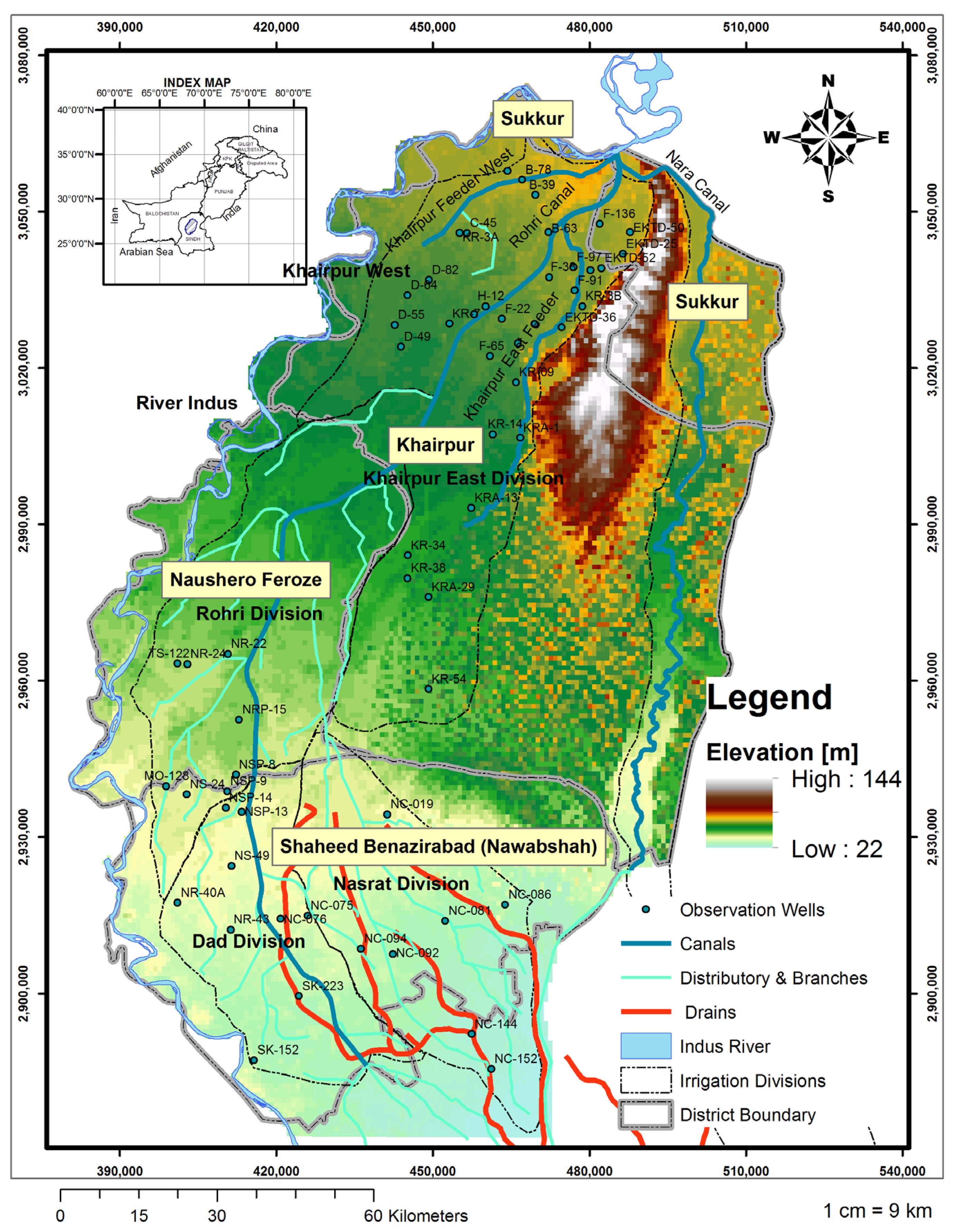
3.1. Study Area

The study area chosen is the Northern Rohri Canal Command Area (CCA), supplied from the left bank of Sukkur Barrage, which covers an intensively cultivated area across the districts of Sukkur, Khairpur, Naushero Feroze, and Shaheed Benazirabad (Figure 1). The study area has four major canals and is divided into five irrigation divisions, i.e., Khaipur West, Khairpur East, Rohri, Dad, and Nasrat divisions. Surface irrigation is the main source and groundwater is secondary but significant, especially between the Indus River and Rohri Canal. The geographical region of the study area is mostly arid and semi-arid, with low annual rainfall and higher evapotranspiration rates, and where temperature increments are expected to be greater than average. May and June have maximum temperatures which can exceed 45 °C, while January is considered the coldest month when temperatures can go below 10 °C. Most rainfall occurs in the months of July, August, and September, with mean annual rainfall ranging between 100 mm to 200 mm. An increasing shortage of surface water has led to a dramatic increase in groundwater use. The groundwater in the area ranges from fresh along the Indus River to marginally fresh and saline across the CCA, dictating where groundwater is likely to be used for irrigation.

3.2. Input Data

Table 1 shows the input dataset used in the study, and a description of the preprocessing of the raw dataset is provided below for acquiring the final data used to model the groundwater system.

3.2.1. Aquifer Properties

A database of 163 bores with logs was compiled from sources provided by Sindh Irrigation Department (SID), WAPDA’s SCARP Monitoring Organization (SMO), and from various previous field studies. These logs were scanned, georeferenced, and compiled in a lithology database. The borelogs, including additional logs from drilling undertaken in our case study sites, were used to estimate hydraulic conductivity, specific yield, specific storage, and porosity.

3.2.2. Precipitation and Temperature

Average monthly temperature and precipitation data over ninety years (2010–2099) for Sindh were acquired from the Numerical Modelling Group of Research and Development Division, Pakistan Metrological Department (PMD). In the current study, RCP4.5, and RCP8.5, both medium and high-end scenario were used. Details for processing methods of the climate dataset can be found in [27].

3.2.3. Evapotranspiration

The number of weather stations with long-term or multi-parameter data records in the Indus Basin is limited and the climate data in much of the region are limited to maximum and minimum temperatures, and rainfall. For our study, we therefore used the Blaney–Criddle Equation (1) to calculate potential evapotranspiration (ETo) using temperature estimated for RC 4.5 and RCP 8.5 scenarios. This is a temperature-based method and can be calculated from the mean temperature as a function of latitude and longitude (see Equation (1)). These data were re-gridded on the groundwater model grid of 1000 m by 1000 m using kriging interpolation.
E T o = p 0.46 T m e a n + 8
where ETo is the reference crop evapotranspiration (mm/d); T(mean) is the mean daily temperature (°C); and p is the mean daily percentage of annual daytime hours.

3.2.4. River and Drainage Properties

The river, canal, and drainage aquifer interaction can be represented by the conductance such that the seepage from/to the river is proportional to the head in the river stage and head in the aquifer cell. In order to define the conductance, river, canal, and drainage hydraulic properties at the main regulators and control sections were collected from SID. These were digitised and interpolated for model cells.

3.2.5. Groundwater Pumping
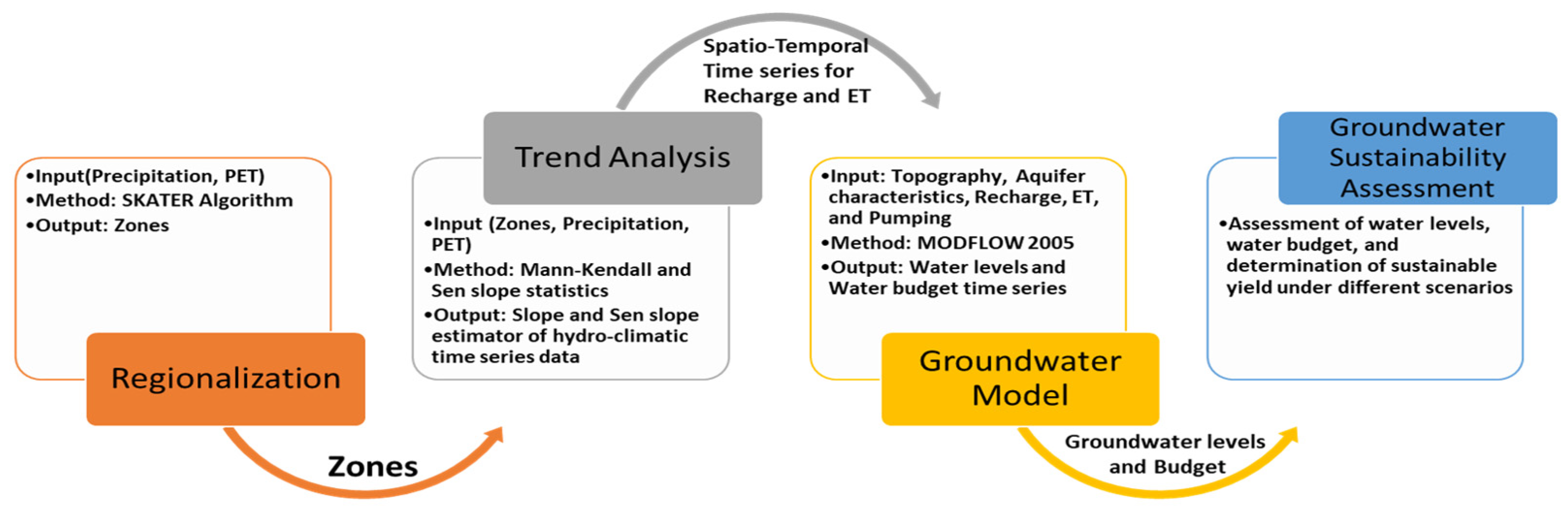
In order to estimate the pumping, a survey was conducted to estimate a density of 5 wells per square kilometre. Most of the private tube wells have a capacity of 1–2 cusecs and pump for an average of 8 h per day. At the tail reaches, groundwater was the sole source of irrigation, and at the mid reaches, farmers used groundwater during periods of surface water shortages.

3.3. Methods

Figure 2 shows the flow chart of the overall methodology. In the first step, climatic regionalisation was carried out for Sindh using Spatial K’luster Analysis using the Tree Edge Removal (SKATER) algorithm [28]. In the second step, trend analysis was performed using Mann–Kendall and Sen’s slope statistics on datasets of precipitation and potential evapotranspiration (PET) for 2010–2099 [29,30]. In the third step, a groundwater flow model using MODFLOW 2005 [31] was calibrated for the study area from October 2010 to April 2014 and simulated until 2047 for generating future water level and budget timeseries. Then, a detail groundwater sustainability assessment was performed using these simulated timeseries of water level and water budget.

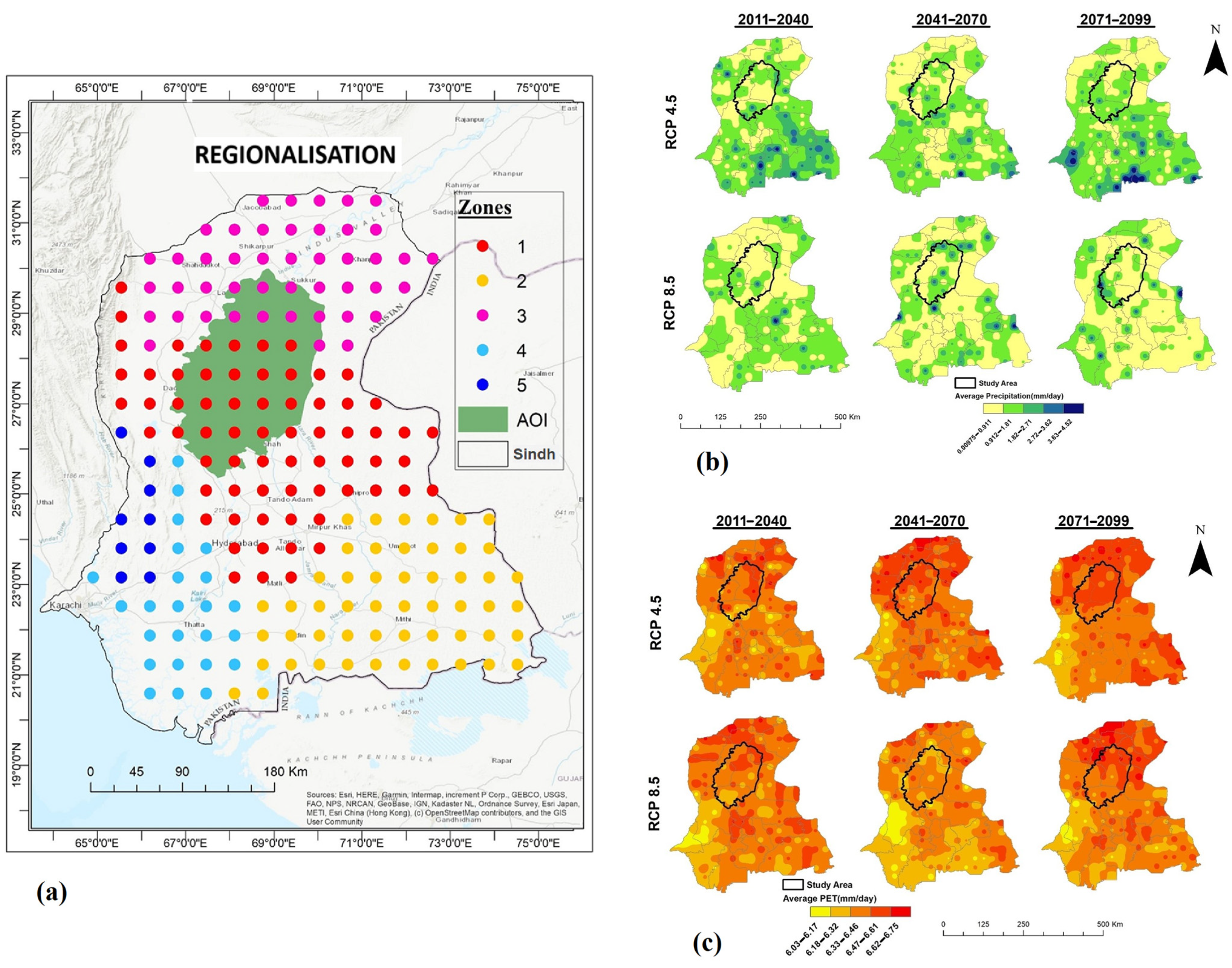
3.3.1. Climate Regionalisation

Regionalising is a valuable technique used frequently in disciplines dealing with large spatial datasets. The goal is to preserve the patterns in the dataset and produce homogeneous and contiguous clusters. The SKATER method [28] was chosen to regionalise Sindh based on projected annual average precipitation and potential evapotranspiration. Its efficiency for regionalisation is because it “combines the use of a minimum spanning tree with combinational optimisation techniques” [28] (p. 809). SKATER represents the objects as graphs that captures adjacency relationships among objects as connections.

3.3.2. Trend Analysis

The Mann–Kendall trend [29] was used to detect any statistically significant trends in precipitation, potential evapotranspiration, and droughts in the future due to climate change. This is a non-parametric test and suitable for those data series where the trend is assumed to be monotonic (i.e., the trend is continuously increasing or continuously decreasing). The test was conducted on a significant level α: 0.05, meaning that there is a 5% probability that the values are from a random distribution, and with that probability, it would be erroneous to reject the null hypothesis (Ho) of no trend. For prediction of the magnitude of the true slope of hydro-climatic time series data, a non-parametric Sen’s slope estimator [30] method was used.

3.3.3. Groundwater Flow Model Development

Water balance assessment was performed via calibration of the groundwater flow model (i.e., MODFLOW 2005 [31]) from October 2010 to April 2014. A monthly water balance was quantified. MODFLOW 2005 uses a continuity equation for water balance (Equation (2)) and a finite difference scheme to solve it numerically:
x k f x h x + y k f y h y + z k f z h z = S o h t + W o
where h = hydraulic head; k = permeability; So = storativity; and Wo = source/sink

Model Conceptualisation and Discretisation

The conceptualisation of the various components of this hydro system is shown in Figure 3. We considered a two-layered aquifer system. The top of Layer 1 is defined by the surface topography obtained from NASA’s surface radar topography mission’s (SRTM) digital elevation model (DEM), which was upscaled to the model grid. The top layer, which extends from the surface to approximately 35 m, is an unconfined layer that includes the Indus River, canals, drains, and shallow private tubewells. The thickness of Layer 2 is between 22 and 306 m, which varies based on the bottom of the aquifer as defined by borelogs. This layer includes deep private tubewells, as well as deep scavenger tubewells, which extract groundwater for disposal into drains. These layers also interact through leakage between them.
The sub-regional model of Sindh is bounded between 376,000 and 523,000 metres east and between 2,872,000 and 3,078,000 metres north. The spatial grid of the model is 1000 m (east) by 1000 m (north) size, with 206 rows and 147 columns. A monthly stress period divided into three time steps was considered for temporal discretisation. The model was calibrated from October 2010 to April 2014 to cover the Rabi and Kharif cropping seasons. Then, the model was simulated through to 2047 for impact assessment of climate change on the groundwater budget. Initial heads were assigned using the SMO dataset post-2015, and point data were interpolated on the model grid using kriging interpolation.

Aquifer Parameterisation

Aquifer parameterisation was performed for two-layer conceptualisation. Based on the material appearing in the borelogs, an initial value was assigned from the standard values for the material, and then kriging interpolation was performed to generate the gridded values. Based on the initial values, the distribution of conductivity and specific yield values is generally higher throughout the study area. There is also a prominent low value zone in the northeast section of the model which coincides with the outcrop areas. Table 2 shows the ranges for the initial values of the parameters. Zonation and adjustment were performed on these initial values during the calibration.

Initial and Boundary Conditions

Initial water levels were assigned based on the initial values for October 2010. Initial water levels are generally shallow in the study area, particularly along the major canals. Therefore, direct evapotranspiration (EVT) from groundwater is expected to be high. In order to capture this phenomenon, evapotranspiration boundary condition based on extinction depth was applied. Monthly data was used for each stress period in the study area, and temporal EVT rates obtained by multiplying potential EVT with crop coefficients were used as a model input. In June and July, maximum EVT rates exceeded 300 mm per month, and varied spatially, with highest values occurring from farm fields. The extinction depth was estimated by using 163 borelogs from the districts of Sukkur, Khairpur, Naushero Feroze, and Shaheed Benazirabad and interpreting the near surface borelog. The extinction depths assigned to each log were adopted from [32]. Major contributions to recharge are from rainfall and irrigation, so a recharge boundary was assigned to quantify these. This was estimated by aggregating recharge from rainfall, canal irrigation, and tubewell irrigation. Basin and furrow irrigation methods are widely used for supplying water to wheat, cotton, vegetable, fruit, and fodder crops during Rabi and Kharif seasons in the study area. The irrigation water supply of the canal command area was estimated for the modelled area on a monthly basis. Since surface irrigation methods are deemed to be 40 to 60 percent efficient, it was estimated that 50 to 60 percent of irrigation water in the modelled area contributed to the aquifer as recharge. The amount was adjusted spatially and temporally during the calibration process. Based on the water supply, each grid cell was assigned returns from irrigation for each monthly stress period.
The river and canals were taken as river boundary cells. The river and canal system in the model is defined by segmenting the river and canal into reaches, such that each reach resides in a single cell so that the area required for calculating conductance is taken for each grid cell. The thickness of bed material (m) is assumed to be 1, with riverbed conductivity included as a model calibration parameter. A similar approach was taken for the drainage boundary.

Calibration

Calibration is a process of varying the quantity and spatial distribution of uncertain model parameters within a probable range until a sufficient consistence of modelled and measured data is achieved. The procedure involves adjusting aquifer hydraulic properties, storage, boundary conditions, and system stresses (recharge, evaporation, river and canal–aquifer interactions) such that the model is capable of simulating both spatial and temporal responses. In this study, the strategy we adopted for calibration involved the following:
  • In Step 1, we divided the aquifer into different zones based on the aquifer properties in the area. Zones were defined based on interpretation of aquifer parameters, and then units with similar properties were grouped.
  • Each unit was assigned a zone number, in which a multiplier was used to adjust the input parameter values.
  • In Step 2, we divided the model domain into different recharge/discharge zones based on irrigation divisions in the model domain. A multiplier was assigned for each parameter to adjust the sink and source terms in each zone, including: (i) rainfall recharge; (ii) irrigation recharge; (iii) evapotranspiration; and (iv) pumping.
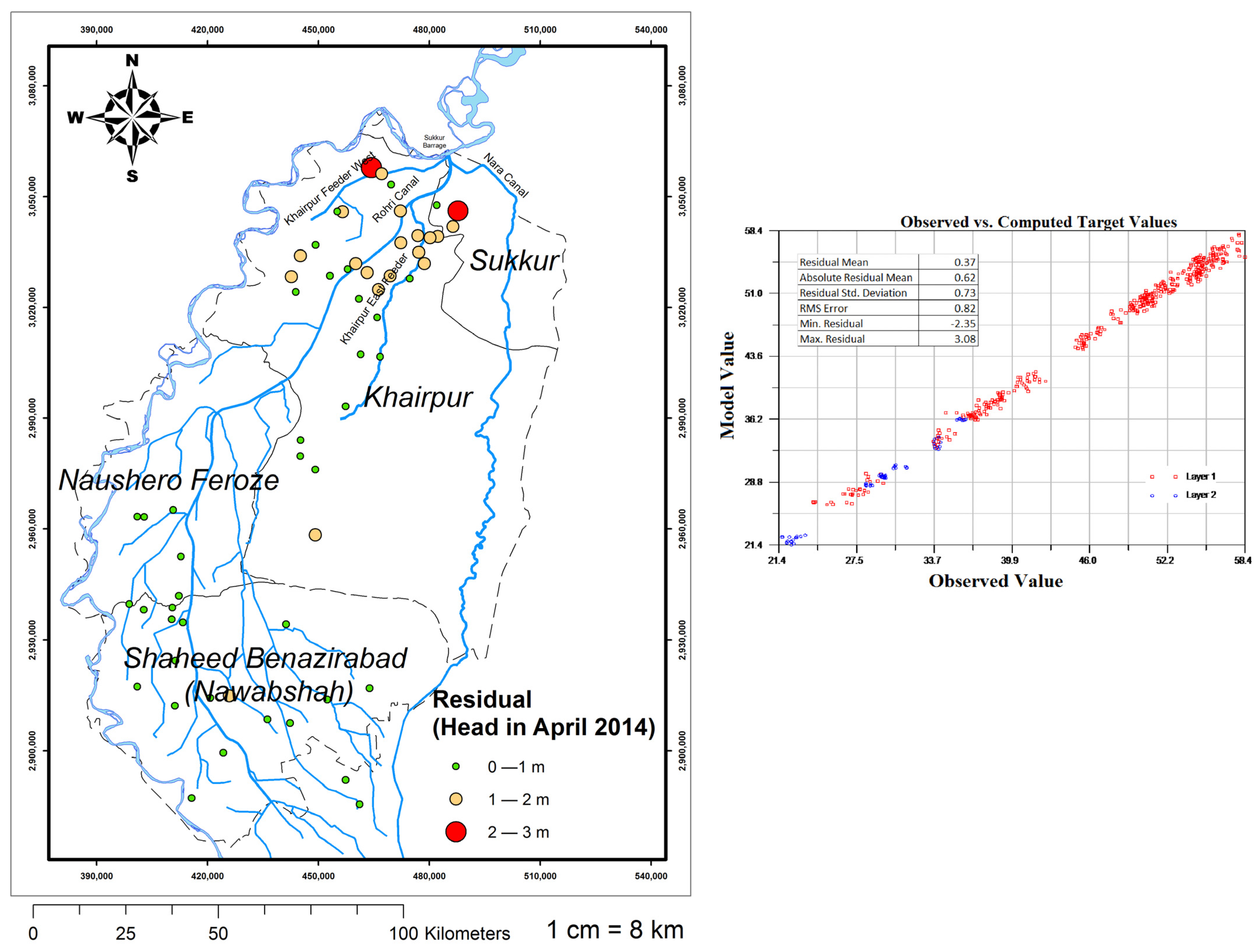
  • Fifty-nine observation wells were considered for calibration to compare the observed versus simulated water heads. Model calibration was performed for 42 stress periods from October 2010 to April 2014. The head measured in October 2010 (post-monsoon) was taken as the initial head condition. Observed heads were arranged for the post- and pre-monsoon season for each year from 2010 to 2014.

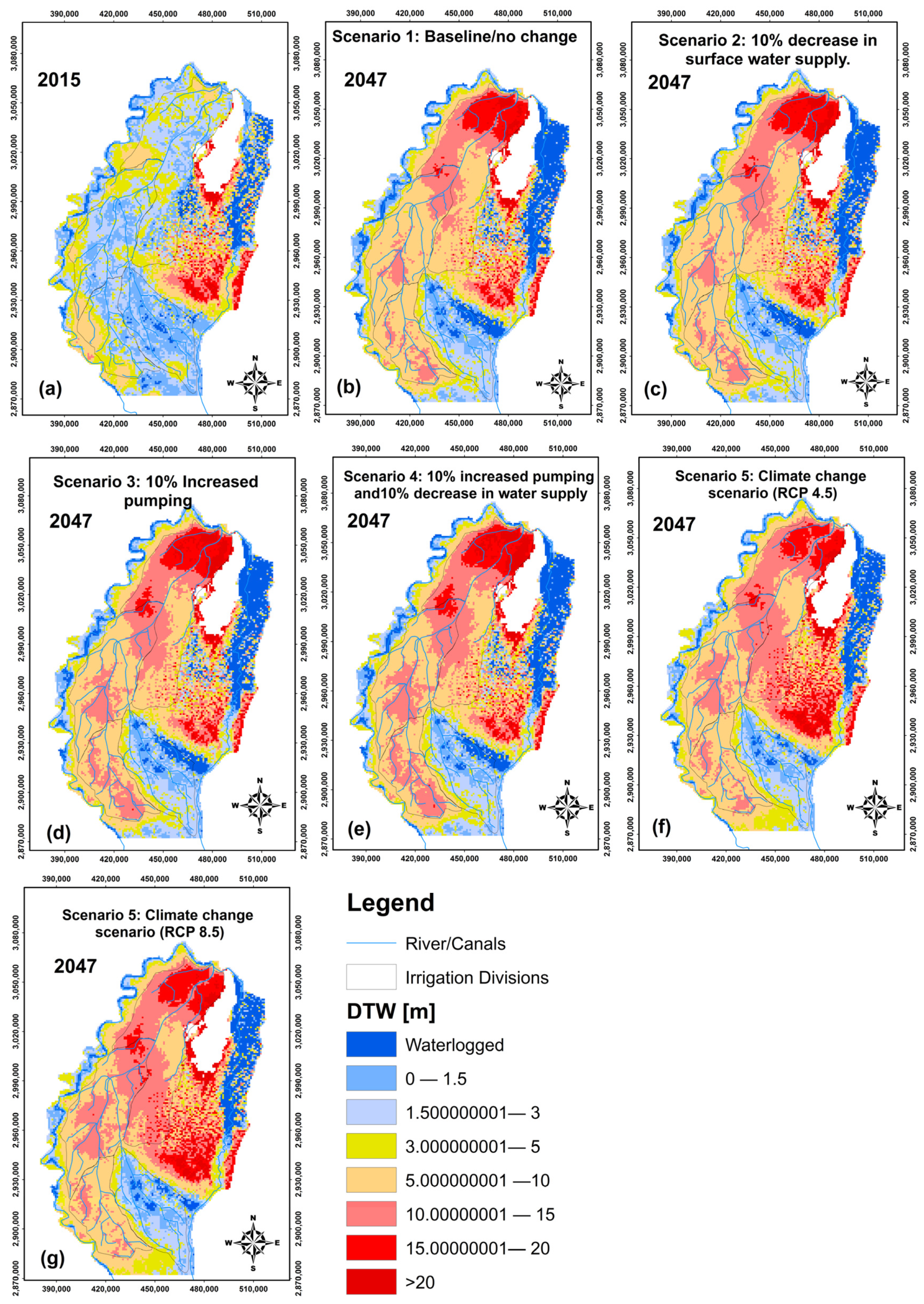
3.3.4. Scenario Assessment

Scenario assessment was performed to evaluate the impact of policy intervention to ensure the sustainable use of groundwater in Sindh. The starting point for these scenarios was the initial head conditions observed in October 2010. The following scenarios were assessed to establish future management policy for sustainable use of groundwater:
  • Scenario 1: Baseline/no change. This scenario assumes that pumping will remain the same as for the calibrated model and is used as a base case to compare with other scenarios.
  • Scenario 2: 10% decrease in surface water supply. This scenario was developed in consultation with SID to assist in understanding its impact on freshwater zones. In this scenario, water supply in the early Kharif period (i.e., April to July) was reduced by 10% of historical amounts.
  • Scenario 3: 10% increased pumping. In this scenario, pumping was increased from the freshwater zone in the same early Kharif period to help identify threshold depth and time scale of depletion, thus helping to set extraction limits for the freshwater lens.
  • Scenario 4: 10% increased pumping and 10% decrease in water supply. In this scenario, pumping was increased for freshwater zone while overall surface water supply was decreased for the early Kharif period to depict a water shortage scenario.
  • Scenario 5: Climate change scenarios. Two scenarios were created where water balance assessment was performed using RCP 4.5 and RCP 8.5 time-series climatic predictions input data.

4. Results

4.1. Regionalisation

Given the significant climate variability across Sindh, the province was divided into five homogenous regions using the SKATER algorithm, drawing on two factors: the spatial contiguity of the dataset, and similarity of key parameters, being the average annual precipitation and PET. These five zones are shown in Figure 4a. Zone 1 (Central) covers the Khairpur, Naushero Feroze, Shaheed Benazirabad, Sanghar, Hyderabad, Dadu, Tando Allahyar, and Matiari districts. Zone 2 (South-Eastern) includes the desert districts of Umar Kot, Badin, and Tharparkar. Zone 3 (Upper) includes districts with high temperatures like Kashmore–Kandhkot, Jacobabad, Ghotki, Sukkur, Shikarpur, Larkana, and Qambar Shahdadkot. Zone 4 (South-Western) contains the districts of Sujawal, Thatta, and lower parts of Karachi. Zone 5 (West) includes Jamshoro and upper parts of the Karachi district. The following sections provide the statistical analysis of spatiotemporal variability for the two climate parameters. The focus of the study is on the intensively cultivated areas of northern Rohri, which includes the Central and Upper Zones (1 and 3).

4.2. Spatiotemporal Precipitation Trends for Northern Rohri CCA

Tables for precipitation trend analysis results are provided as Supplementary Material. The analysis shows future precipitation increasing in the south-eastern Zone 2 for both RCP scenarios, especially in the Tharparkar district. Our study area of interest (AOI), the Northern Rohri CCA, shows a non-significant increasing trend of precipitation in both scenarios. The RCP 4.5 scenario analysis for Zones 1 and 3, wherein our study area is located, reveals that maximum average precipitation (mm/day) and standard deviations are high for the months of July, August, and September, especially for Zone 1 (the southern areas of our study area). The Mann–Kendall (MK) monthly precipitation trends for both these zones show an increasing trend for March and for September to December and a decreasing trend for other months. There is a significantly decreasing trend early in the monsoon period (July and July) for both zones, which suggests a delay in the monsoon period that historically occurs from June to September towards the months of August to October. Sen’s slope (Q) analysis shows the magnitude of the trends in mm/year, which for both zones are significantly negative for June to August, but positive for September to November. According to the RCP 8.5 high emission scenario analysis, the maximum average precipitation and standard deviations are again high in both Zones 1 and 3 for the months of August and September, and mostly higher than for the RCP 4.5 scenario. The Mann–Kendall monthly precipitation trends show an increasing trend for a longer period from January through to March as well as for September to December for both zones. The trend for the RCP 8.5 scenario again suggests a delay in the monsoon with a significantly decreasing trend in participation for June and July, coupled with a highly significant increase in future winter precipitation. Sen’s slope (Q) analysis reveals that the magnitude of precipitation trend in the first five months of the year is approximately zero, significantly negative for June to August, and significantly positive for September to December.

4.3. Spatiotemporal Potential Evapotranspiration Trends (PET) for Northern Rohri CCA

After calculating PET using Blaney Criddle’s equation, the spatiotemporal trends for Sindh were analysed. Tables for PET trend analysis results are provided as Supplementary Material. Significantly increasing PET trends are observed in Zone 3 for all three future periods shown, and a generally increasing trend is observed for our study area under both scenarios. Under the RCP 4.5 scenario, the PET trends for Zones 1 and 3 greatly increased over time in summer, while they decreased during winter months. The Mann–Kendall (Z) and Sen’s slope (Q) analyses both show negative PET trends from March to May for both zones.
Under the RCP 8.5 scenario, PET is at its maximum in June and July, with a high increase in PET across the summer months. The Mann–Kendall and Sen’s slope analyses reveal negative trends for just two months (March and April), with a highly increasing PET trend for all remaining months.

4.4. Groundwater Model Calibration

Figure 5 shows spatial calibration for 59 observation points obtained at the end of the model calibration period (April 2014). At the end of the model calibration, most (39) piezometers in the study area showed a low residual value (i.e., a difference between the observed and the simulated water levels) in the range of 0–1 m, with 20 having a higher residual, mostly located towards the northern end (18 in the range of 1–2 m, and two greater than 2 m). A root mean square value of 0.82 and absolute mean error of 0.62 m were obtained, suggesting an acceptable calibration of the simulated water levels over the model domain.
The observed levels during the calibration in each irrigation division showed groundwater level declines in response to pumping as well as recovery following monsoonal rainfall recharge. Almost all pumping in the model domain is from the shallow (Layer 1) watertables that had developed due to rainfall, canal seepage, and irrigation return flows. These shallow freshwater lenses provide an opportunity for farmers to extract groundwater for irrigation. The bore responses show that water levels are either stable or declining by less than 1 m during the calibration period (October 2010 to April 2014). This result is reassuring given that approximately 3 BCM of groundwater is used annually in this area by farmers as supplementary irrigation when surface water supplies are inadequate. However, improved monitoring is required in areas with declining water levels to ensure the water quality of the freshwater lens does not decline at current extraction rates. Access to this groundwater allows farmers to maintain crop productivity and is an important supplementary source safeguarding their livelihoods.

4.5. Modelled Water Balance

The modelled water balance we undertook for Layers 1 and 2 for the period 2010 to 2014 confirms that the major inflow to Layer 1 is recharge (3.943 BCM) followed by an upward flow from Layer 2 (2.051 BCM), with the Indus contributing 1.16 BCM. Recharge from the Indus has been curtailed in recent times due to the construction of levies to control flooding during high flows, and significant upstream diversions. In its natural state, the Indus would have more frequently breached its banks during monsoon floods. The reduced recharge from the river has now been supplemented by increased recharge from canal seepage and irrigation. Significant outflows from Layer 1 are a result of pumped extractions (2.942 BCM) and the downward flow of groundwater to Layer 2 (2.48 BCM). The overall movement of water between Layers 1 and 2 indicates that Layer 1 is, on balance, contributing to inflows to Layer 2. It is important to ensure that an overall reversal of these gradient flows does not occur as this would lead to salinity transport from the lower layer to the upper layer, with the increased salinity in the upper layer likely to reduce crop productivity and thus undermine farming family livelihoods. The other significant loss from the top layer is through evapotranspiration (1.606 BCM), indicating the prevalence of shallow watertables in the model area.
In addition to the downward inflows to Layer 2 from Layer 1, there is a small amount of Layer 2 recharge occurring near the Kirther formation outcrop in the Khairpur district. However, the largest outflows from Layer 2 are actually upward flows to Layer 1, indicating that, in some areas of the model, groundwater pumping has become so significant that gradients between the layers may have reversed and an upward flow is occurring. This will need to be managed to avoid upward transport of deeper dissolved salts, reducing the useability of freshwater lenses in the upper layer. The other major outflow from Layer 2 involves boundary outflows (0.859 BCM) along the model’s eastern boundary towards the Thar Desert. There is also a small amount of pumping by SCARP tubewells from Layer 2 (0.307 BCM) which is used for vertical drainage. This is where groundwater from the deeper layer is pumped into drainage channels so that the saline water can be removed via the Left Bank Outfall Drain (LBOD) to the sea.

4.6. Modelled Water Balance for the Longer-Term Scenario

The water balance for the scenarios based on historical climatic cycles is presented in Table 3. All values are in BCM and are averaged over the 32 years of simulation. In the baseline scenario, the two major components of the water balance inflows are recharge from irrigation and river/canal leakages (4.282 BCM). The major outflow is from wells (3.619 BCM) and evapotranspiration (1.754 BCM). The net loss for the baseline scenario is −1.244 BCM, which is equivalent to a 73 mm/year decline in average water levels. Reducing canal supplies by 10% during early Kharif (Scenario 2) will not have a significant change in the average groundwater recharge over the simulation period as compared with the baseline scenario. Net storage will only decrease slightly from −1.244 (baseline) to −1.343 BCM (Scenario 2). The 10% increase in pumping scenario will reduce net storage from −1.244 to −1.436 BCM, which represents an almost 15% decline in net storage compared with the baseline scenario. If both a 10% increase in pumping and 10% decrease in recharge were to take place simultaneously (Scenario 4), then the net loss in storage for the model increases from −1.244 (baseline) to −1.535 BCM, which is equivalent to a decline in water levels of 90 mm per year.
Under the climate change scenarios RCP 4.5 and RCP 8.5, the net loss in storage increases substantially to −2.815 and −2.214 BCM, respectively. This outcome results from the projected lower rainfall and higher temperatures, which would drive higher evapotranspiration, especially in the RCP 8.5 scenario. The recharge in the system decreases from 3.944 BCM to 3.769 (for RCP 4.5) and 3.732 BCM (for RCP 8.5) compared with the baseline scenario. In response to high projected temperatures, outflow due to evapotranspiration is seen to increase by approximately 36–38% in RCP 4.5 and RCP 8.5 scenarios compared with the baseline scenario. All other water balance terms remain unchanged, except drainage outflows, which reduce from 0.47 (baseline) to 0.27 (RCP 4.5 and 8.5) due to a lowering of the watertables from higher rates of evapotranspiration.

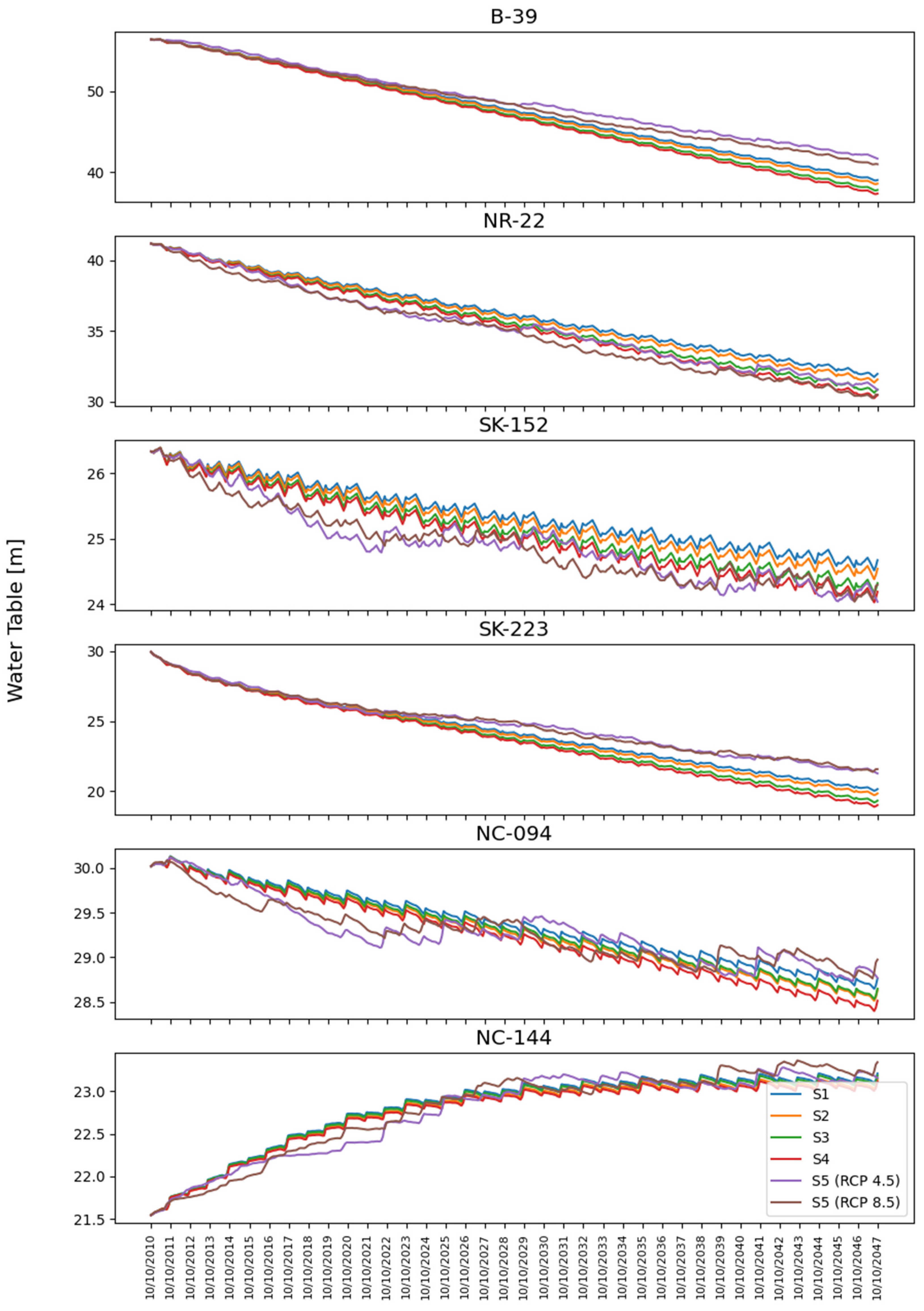
4.7. Water Level Assessment under Different Scenarios

The spatial distribution of groundwater depths for the calibrated model and various scenarios is shown in Figure 6, with modelled temporal trends in watertable levels for selected piezometers shown in Figure 7. Depth to water (DTW) levels are divided into categories: waterlogged (dark blue in Figure 6); shallow watertables (0–1.5 m and 1.5–3.0 m—lighter blue); moderate water levels (3.0–10 m—yellow and orange); and deep water levels (>10 m—pink and red). For 2015, across all canal command areas, DTW is in the shallow or moderate watertable category. Shallow watertables can be seen at the head and mid reaches of distributaries, whereas DTW falls to moderate levels at the tail reaches, especially for canal command areas near the Indus River. This is because tail reaches near the Indus River comprise areas with more substantial reserves of non-saline groundwater that is extensively used for irrigation. DTW levels in non-irrigated areas are deeper as these areas are distanced away from where most of the recharge occurs (i.e., from irrigation return flows, canal leakage, and river inflows). In non-irrigated areas, the only source of recharge is from surrounding boundaries or from precipitation, which is minimal. For the baseline scenario, DTW levels by 2047 in the Khairpur East (KE) irrigation division are expected to change from moderate to deep, indicating declining trends. Most of KE will have DTW levels between 10 and 15 m, except the riverine area, which will maintain its moderate water levels. Such a large decline in DTW levels will deteriorate groundwater quality significantly. It is worth noting, however, that, in the simulation, the extent of groundwater extraction was not constrained. Realistically, farmers will stop pumping groundwater when its quality makes it unusable. If farmers continue pumping beyond this limit due to water shortages, then the resulting increased accumulation of salts in the root zone will have an adverse impact on agriculture land and productivity.
Climate change scenarios also showed lowering trends for DTW, but the gradient of decline was less constant (see purple and brown lines in Figure 7). For two monitoring locations (SK-152 and NC-094), the DTW trends over time sometimes increased but mostly decreased, with the DTW in 2047 ending up similar to that for the baseline scenario. For two other monitoring locations (B-39 in the north and SK-223 in the south), the gradient diverges from that of the baseline scenario after the year 2028, showing a less pronounced decline, and DTW for the climate change scenarios, ending up 5 m higher than for the baseline scenario. One monitoring location in Nasrat irrigation division (NC-144) revealed a reverse trend, with DTW ending up at a higher level for all scenarios due to very low groundwater extractions at that location, an area of flat topography. This trend indicates that drainage will play an important role in such areas to minimise waterlogging from rising watertables and thus maintain agricultural productivity.

5. Discussion

Given climate variability in Sindh, the region was divided into five contiguous zones using the SKATER algorithm technique based on two climate parameters: precipitation and potential evapotranspiration. Analysis of the zones generated for the Northern Rohri CCA showed a negative trend for monsoon precipitation for both RCP 4.5 and RCP 8.5 climate scenarios and a delay in monsoon occurrence. Potential evapotranspiration showed a decreasing trend in winter season and a significantly increasing trend in summer in both scenarios.
The groundwater budget for the Norther Rohri CCA model indicated that river–aquifer connectivity, canal recharge, evapotranspiration, and groundwater pumping for irrigation were significant components for the upper layer of the aquifer, and, for the lower layer, interlayer leakage and pumping of saline water are important considerations. The results showed that the net loss in storage over the simulation period from October 2010 to April 2014 was −1.04 BCM/year. The net decline in storage in Layer 1 was −0.374 BCM and −0.665 in Layer 2. The sustainable yield was estimated at 3 ± 0.3 BCM to allow for adaptive management during times of drought and inadequate surface supplies and to safeguard livelihoods. For the RCP 4.5 scenario, the net loss in storage over the simulation period for 2010–2047 was −2.185 BCM/year (compared with −1.04 BCM/year for the baseline scenario). The net decline in storage was −0.625 BCM/year in Layer 1 and −1.558 BCM/year in Layer 2. For the RCP 8.5 scenario, the net loss in storage over the simulation period (2010–2047) was −2.214 BCM/year as compared with the baseline scenario (−1.04 BCM/year).
Groundwater level trends show an overall declining trend. This is concerning given that the freshwater lens in Sindh is a few metres thick and overlies deeper saline groundwater. A lack of access to groundwater in the future will force farmers to reduce cropping intensity with consequent adverse impacts on food security and the need to increase food imports. Continued use of groundwater in this environment will need to be accompanied by investments in water productivity to minimise adverse impacts of waterlogging and salinisation, and to preserve the freshwater lenses for the future of groundwater irrigation in Sindh. As climatic conditions become more challenging, management rules will be needed for pumping from the freshwater zones in the upper layer to avoid salinisation of the aquifer.
Our regionalised analysis, as exemplified by the Norther Rohri CCA groundwater model and budget, also provides implications for strategies that can be adopted to achieve the above-referred measures needed to secure groundwater yields that are sustainable and to avoid waterlogging and salinisation. This is the first time an estimate of sustainable yield has been made for this important agricultural region of Sindh and this will provide the irrigation authorities with guidance on groundwater planning, which in the past has largely been ignored. Our approach has led to recommendations that groundwater management strategies be developed at regional (irrigation division) scales [33,34], drawing on similar strategies adopted in Australia. In Australia, long-term sustainable yields are determined for specific groundwater management areas through agreement with users [35,36]. These area-specific sustainable yields can be revised after 5 to 10 years of application according to agreements that have been made with groundwater users, or in response to droughts or increased development of groundwater use in the management area.
Such a regionalised process could be developed for groundwater management areas in Sindh, which would rely on having revised and improved groundwater models in place. These would enable SID, as the manager of these water resources, to develop an improved understanding of risks to groundwater from overexploitation and salinity intrusion, as well as to support SID’s capacity to meet objectives of both the National and Sindh Water Policies. The importance that the National Water Policy has placed on groundwater will require significant investment in building capacity within SID to improve management of groundwater. With effective stakeholder engagement, this will ensure an equitable framework can be developed for sustainable management of groundwater [36,37].
Setting an allocation limit based on an assessment of sustainable yield does not necessarily mean hotspots will not occur, particularly in groundwater systems in the LIB. With increasing pressures on groundwater resources, resource managers recognise that despite an overall sustainable yield for a groundwater management area, localised areas of declining groundwater levels and quality would require water level response management, especially for systems nearing full allocation [35]. Future management of groundwater in the Indus Basin will thus require improved strategies focused on hotspots where sustainable future use of groundwater is critical.
The model simulated declining groundwater levels across all five SID divisions that traverse the area. Expansion of groundwater abstractions in all divisions except Nasrat should be monitored meticulously, with allocation limits adopted in consultation with users to manage hotspots and to ensure groundwater availability with suitable quality is maintained for future users. Most of the Nasrat division has poor groundwater quality, so the likelihood of additional pumping is low. However, shallow watertable management may be required to limit the spread of waterlogging and salinity. This could be achieved by adopting crops that use less water, improving irrigation management practices, and land management. Systematic monitoring of groundwater in the Northern Rohri CCA is essential to allow irrigation agencies and farming communities to improve the management of groundwater and to allow model extension to account for the increased number of tubewells and ensure the robustness of calibration.

6. Conclusions

The canal command areas supplied from the left bank of the Sukkur Barrage is considered the food basket for the people of Sindh province. Farmers across these areas add substantially to the provincial and national economy through their agricultural activities while also supporting the livelihoods of their families by making good use of the human, land, and water resources available to them. It is important, therefore, that use of these resources is managed sustainably, especially given the projected impacts of climate change, which is expected to be felt especially severely by Pakistan [11]. Our above regional assessment of the impacts from climate change and other factors on groundwater offers tangible benefits for planning and managing the resource for the Northern Rohri CCA in particular. Based on the assessment, it can be concluded that Sindh can be divided into five zones for future climate change assessment. In Upper Sindh and Central Sindh, there will be no significant changes in precipitation but evapotranspiration will increase. This increase will affect the groundwater use zones in the area. In order to sustain the groundwater resources of the Northern Rohri CCA, which is the most important groundwater extraction zone, a sustainable yield would need to be no greater than 3 ± (0.3) BCM. In order to sustain agriculture land in shallow zones, we recommend that an allowance of 10% of the sustainable yield (0.3 BCM) would allow farmers to increase extraction during drought years, which could then be replenished when rainfall and surface water flows increase. As the impacts of climatic change intensify, groundwater managers will need to collaborate with users to modify how much is pumped from upper-level freshwater zones to avoid increased salinisation of the aquifer.

Supplementary Materials

The following supporting information can be downloaded at: https://www.mdpi.com/article/10.3390/su16010441/s1.

Author Contributions

Conceptualisation, J.F.P., M.M. and W.A.; methodology, J.F.P. and W.A.; validation, W.A., J.F.P. and M.S.E.; formal analysis, W.A. and S.A.; investigation, W.A., J.F.P. and S.A.; resources, A.L.Q.; data curation, S.A., W.A. and G.H.D.; writing—original draft preparation, W.A. and S.A.; writing—review and editing, M.M., J.F.P. and W.A.; visualisation, S.A., G.H.D. and W.A.; supervision, A.L.Q., G.H.D. and M.S.E.; project administration, A.L.Q.; funding acquisition, J.F.P. and M.M. All authors have read and agreed to the published version of the manuscript.

Funding

This research was funded by the Australian Centre for International Agricultural Research (ACIAR) (Project No. LWR-2015-036), with additional funds provided by Charles Sturt University.

Data Availability Statement

Model data and code can be made available on request.

Acknowledgments

We acknowledge that material and data were provided by SCARP’s Monitoring Organization (SMO), WAPDA, Pakistan, and Sindh Irrigation Department, Government of Sindh, Pakistan. We also acknowledge the Numerical Modelling Group of Research and Development Division of the Pakistan Metrological Department (PMD) for providing access to precipitation and evapotranspiration data for Pakistan. Finally, we acknowledge with much gratitude the support and guidance provided by Evan Christen and Robyn Johnston, ACIAR’s Water Research Program Managers, who had a deep understanding of the importance of groundwater in Pakistan.

Conflicts of Interest

The authors declare no conflict of interest.

References

  1. Qazi, M.A.; Khattak, M.A.; Khan, M.S.A.; Chaudhry, M.N.; Mahmood, K.; Akhter, B.; Iqbal, N.; Ilyas, S.; Ali, U.A. Spatial distribution of heavy metals in ground water of Sheikhupura district Punjab, Pakistan. J. Agric. Res. 2014, 52, 99–110. [Google Scholar]
  2. Qureshi, A.S.; Gill, M.A.; Sarwar, A. Sustainable groundwater management in Pakistan: Challenges and opportunities. Irrig. Drain. 2010, 59, 107–116. [Google Scholar] [CrossRef]
  3. Qureshi, R.H.; Ashraf, M. Water Security Issues of Agriculture in Pakistan; Pakistan Academy of Sciences: Islamabad, Pakistan, 2019. [Google Scholar]
  4. Qureshi, A.S. Groundwater governance in Pakistan: From colossal development to neglected management. Water 2020, 12, 3017. [Google Scholar] [CrossRef]
  5. Watto, M.A.; Mitchell, M.; Akhtar, T. Pakistan’s water resources: Overview and challenges. In Water Resources of Pakistan: Issues and Impacts; Watto, M.A., Mitchell, M., Bashir, S., Eds.; Springer: Cham, Switzerland, 2021; pp. 1–12. [Google Scholar]
  6. Khattak, A.; Ahmed, N.; Hussain, I.; Qazi, M.A.; Khan, S.A.; Rehman, A.-U.; Iqbal, N. Spatial distribution of salinity in shallow groundwater used for crop irrigation. Pak. J. Bot. 2014, 46, 531–537. [Google Scholar]
  7. Punthakey, J.F.; Khan, M.R.; Riaz, M.; Javed, M.; Zakir, G.; Usman, M.; Amin, M.; Ahmad, R.N.; Blackwell, J.; Richard, C.; et al. Optimising Canal and Groundwater Management to Assist Water User Associations in Maximizing Crop Production and Managing Salinisation in Australia and Pakistan: Assessment of Groundwater Resources for Rechna Doab, Pakistan; Ecoseal Developments Pty Ltd.: Roseville, Australia, 2015. [Google Scholar]
  8. Watto, M.A.; Mugera, A.W.; Kingwell, R.; Saqab, M.M. Re-thinking the unimpeded tube-well growth under the depleting groundwater resources in the Punjab, Pakistan. Hydrogeol. J. 2018, 26, 2411–2425. [Google Scholar] [CrossRef]
  9. Basharat, M.; Tariq, A.-u.-R. Groundwater modelling for need assessment of command scale conjunctive water use for addressing the exacerbating irrigation cost inequities in LBDC irrigation system, Punjab, Pakistan. Sustain. Water Resour. Manag. 2015, 1, 41–55. [Google Scholar] [CrossRef]
  10. Bhutta, M.N.; Alam, M.M. Prospectives and limits of groundwater use in Pakistan, Groundwater research and management: Integrating science into management decisions. In Proceedings of the IWMI-ITP-NIH International Workshop, Roorkee, India, 8–9 February 2005; Sharma, B.R., Villholth, K.G., Sharma, K.P., Eds.; IWMI: Colombo, Sri Lanka, 2006; pp. 105–114. [Google Scholar]
  11. Eckstein, D.; Hutfils, M.-L.; Winges, M. Global Climate Risk Index 2019. Who Suffers Most from Extreme Weather Events? Germanwatch Briefing Paper: Bonn, Germany, 2018. [Google Scholar]
  12. Parry, M.L.; Canziani, J.P.; van der Linden, P.J.; Hanson, C.E. Contribution of Working Group II to the Fourth Assessment Report of the Intergovernmental Panel on Climate Change 2007; Cambridge University Press: Cambridge, UK, 2007. [Google Scholar]
  13. Crosbie, R.S.; McCallum, J.L.; Harrington, G.A. Diffuse Groundwater Recharge Modelling across Northern Australia. A Report to the Australian Government from the CSIRO Northern Australia Sustainable Yields Project. CSIRO Water for a Healthy Country Flagship, Australia; CSIRO: Canberra, Australia, 2009.
  14. Ashraf, A.; Ahmad, Z. Regional groundwater flow modelling of Upper Chaj Doab of Indus Basin, Pakistan using finite element model (Feflow) and geoinformatics. Geophys. J. Int. 2008, 173, 17–24. [Google Scholar] [CrossRef]
  15. Khan, H.F.; Yang, Y.C.E.; Ringler, C.; Wi, S.; Cheema, M.J.M.; Basharat, M. Guiding groundwater policy in the Indus Basin of Pakistan using a physically based groundwater model. J. Water Resour. Plan. Manag. 2017, 143, 05016014. [Google Scholar] [CrossRef]
  16. Ahmed, W.; Rahimoon, Z.A.; Oroza, C.A.; Sarwar, S.; Qureshi, A.L.; Punthakey, J.F.; Arfan, M. Modelling groundwater hydraulics to design a groundwater level monitoring network for sustainable management of fresh groundwater lens in Lower Indus Basin, Pakistan. Appl. Sci. 2020, 10, 5200. [Google Scholar] [CrossRef]
  17. Chandio, A.S.; Lee, T.S.; Mirjat, M.S. The extent of waterlogging in the lower Indus Basin (Pakistan): A modeling study of groundwater levels. J. Hydrol. 2012, 426–427, 103–111. [Google Scholar] [CrossRef]
  18. Kori, S.M.; Qureshi, A.L.; Lashari, B.K.; Memon, N.A. Optimum strategies of groundwater pumping regime under scavenger tubewells in Lower Indus Basin, Sindh, Pakistan. Int. Water Technol. J. 2013, 3, 138–145. [Google Scholar]
  19. Hunting Technical Services Limited; Sir Mott MacDonald & Partners Ltd. The Lower Indus Report; West Pakistan Water and Power Development Authority: Lahore, Pakistan, 1965.
  20. Bennett, G.D.; Rehman, A.U.; Sheikh, J.A.; Ali, S. Analysis of Pumping Tests in the Punjab Region of West Pakistan, Geological Survey Water-Supply Paper 1608-G, Prepared in Cooperation with the W Pakistan Water & Power Dec Authority under US AID; U.S. Government Printing Ofiice: Washington, DC, USA, 1969.
  21. Sir Mott MacDonald & Partners Ltd. LBOD Stage 1 Project, Mirpurkhas, Pilot Study: Hydrogeology, Special Wells, Preliminary Well Design, Well Numbers and Spacing; Technical Report Annexes 1–6; Mott MacDonald: Croydon, UK, 1990. [Google Scholar]
  22. Bonsor, H.C.; MacDonald, A.M.; Ahmed, K.M.; Burgess, W.G.; Basharat, M.; Calow, R.C.; Dixit, A.; Foster, S.S.D.; Gopal, K.; Lapworth, D.J.; et al. Hydrogeological typologies of the Indo-Gangetic basin alluvial aquifer, South Asia. Hydrogeol. J. 2017, 25, 1377–1406. [Google Scholar] [CrossRef] [PubMed]
  23. MacDonald, A.M.; Bonsor, H.C.; Ahmed, K.M.; Burgess, W.G.; Basharat, M.; Calow, R.C.; Dixit, A.; Foster, S.S.D.; Gopal, K.; Lapworth, D.J.; et al. Groundwater quality and depletion in the Indo-Gangetic Basin mapped from in situ observations. Nat. Geosci. 2016, 9, 762–766. [Google Scholar] [CrossRef]
  24. Iqbal, N.; Ashraf, M.; Imran, M.; Salam, H.A.; ul Hasan, F.; Khan, A.D. Groundwater Investigations and Mapping the Lower Indus Plain; Pakistan Council of Research in Water Resources (PCRWR): Islamabad, Pakistan, 2020.
  25. Alamgir, A.; Khan, M.A.; Schilling, J.; Shaukat, S.S.; Shahab, S. Assessment of groundwater quality in the coastal area of Sindh province, Pakistan. Environ. Monit. Assess. 2016, 188, 78. [Google Scholar] [CrossRef] [PubMed]
  26. Podgorski, J.E.; Eqani, S.A.M.A.S.; Khanam, T.; Ullah, R.; Shen, H.; Berg, M. Extensive arsenic contamination in high-pH unconfined aquifers in the Indus Valley. Sci. Adv. 2017, 3, e1700935. [Google Scholar] [CrossRef] [PubMed]
  27. Burhan, A.; Waheed, I.; Syed, A.A.B.; Rasul, G.; Shreshtha, A.B.; Shea, J.M. Generation of high–resolution gridded climate fields for the Upper Indus River Basin by downscaling CMIP5 outputs. J. Earth Sci. Clim. Change 2015, 6, 1000254. [Google Scholar] [CrossRef]
  28. Assunção, R.M.; Neves, M.C.; Câmara, G.; Da Costa Freitas, C. Efficient regionalization techniques for socio-economic geographical units using minimum spanning trees. Int. J. Geogr. Inf. Sci. 2006, 20, 797–811. [Google Scholar] [CrossRef]
  29. Mann, H.B. Nonparametric tests against trend. Econometrica 1945, 13, 245–259. [Google Scholar] [CrossRef]
  30. Sen, P.K. Estimates of the regression coefficient based on Kendall’s Tau. J. Am. Stat. Assoc. 1968, 63, 1379–1389. [Google Scholar] [CrossRef]
  31. Harbaugh, A.W. MODFLOW-2005, the U.S. Geological Survey Modular Ground-Water Model—The Ground-Water Flow Process; US Department of the Interior; US Geological Survey: Reston, VA, USA, 2005. [Google Scholar]
  32. Shah, N.; Nachabe, M.; Ross, M. Extinction depth and evapotranspiration from ground water under selected land covers. Groundwater 2007, 45, 329–338. [Google Scholar] [CrossRef]
  33. Punthakey, J.; Ashfaq, M.; Allan, C.; Mitchell, M. Improving Groundwater Management to Enhance Agriculture and Farming Livelihoods in Pakistan: Final Report; ACIAR Report No. FR2021-056; Australian Centre for International Agricultural Research: Canberra, Australia, 2021.
  34. Ahmed, W.; Ejaz, M.S.; Memon, A.; Ahmed, S.; Sahito, A.; Qureshi, A.L.; Khan, M.R.; Memon, K.S.; Khero, Z.; Lashari, B.K.; et al. Improving Groundwater Management to Enhance Agriculture and Farming Livelihoods: Groundwater Model for Left Bank Command of Sukkur Barrage in Khairpur, Naushero Feroze, and Shaheed Benazirabad Districts; ILWS Report No 159; Institute for Land, Water and Society; Charles Sturt University: Albury, Australia, 2021. [Google Scholar]
  35. Pierce, D.; Cook, P. Conceptual approaches, methods and models used to assess extraction limits in Australia: From sustainable to acceptable yield. In Sustainable Groundwater Management: A Comparative Analysis of French and Australian Policies and Implications to Other Countries; Rinaudo, J.-D., Holley, C., Barnett, S., Montginoul, M., Eds.; Springer: Cham, Switzerland, 2020; pp. 275–289. [Google Scholar]
  36. Richardson, S.; Evans, R.; Harrington, G. Connecting science and engagement: Setting groundwater extraction limits using a stakeholder-led decision-making process. In Basin Futures: Water Reform in the Murray-Darling Basin; Connell, D., Grafton, R.Q., Eds.; ANU e-Press: Canberra, Australia, 2011; pp. 351–366. [Google Scholar]
  37. Allan, C.; Mitchell, M.; Punthakey, J.F. Institutional pathways for transforming groundwater planning and management: Reflections from Pakistan and Sri Lanka. World Water Policy 2023, 9, 283–668. [Google Scholar] [CrossRef]
Figure 1. Location of the study area and its features (topography, rivers, canals, branches, drainage system, and observation wells).
Sustainability 16 00441 g001
Figure 2. Flow chart for overall methodology.
Sustainability 16 00441 g002
Figure 3. Model conceptualisation and typical cross-section of the model. Red cells are pumping cells, and green cells show river cells. Arrow shows the water balance components.
Sustainability 16 00441 g003
Figure 4. (a) Climate zones produced after running the SKATER algorithm; (b) spatiotemporal pattern of precipitation (mm); (c) spatiotemporal pattern of potential evapotranspiration. AOI refers to the Northern Rohri CCA as our area of interest and is replicated across all maps.
Sustainability 16 00441 g004
Figure 5. Calibration statistics.
Sustainability 16 00441 g005
Figure 6. Spatial distribution of depth to groundwater level from top of natural surface in 2015 for: (a) depth to water level in 2015 for calibrated model; and in 2047 for (b) baseline scenario; (c) 10% decrease surface water supplies; (d) 10% increase in pumping; (e) increase in pumping and 10% decrease surface water supplies; (f) RCP 4.5; (g) RCP 8.5.
Sustainability 16 00441 g006
Figure 7. Simulated heads [mMSL] for selected monitoring points. The locations of these points are shown in Figure 1.
Sustainability 16 00441 g007
Table 1. Summary of datasets, their resolution, and sources used in the study.
MethodDataSpatial and Temporal ResolutionSource
Climatic Regionalisation and trend analysisPrecipitationMonthly, 25 km × 25 kmhttps://www.pmd.gov.pk/rnd/rndweb/rnd_new/climchange_ar5.php
(accessed on 3 January 2024)
TemperatureMonthly, 25 km × 25 kmhttps://www.pmd.gov.pk/rnd/rndweb/rnd_new/climchange_ar5.php
(accessed on 3 January 2024)
Potential EvapotranspirationMonthly, 25 km × 25 kmDerived from Temperature datasets using Blaney-Criddle approach
Groundwater modelTopography90 m × 90 mhttps://csidotinfo.wordpress.com/data/srtm-90m-digital-elevation-database-v4-1/
(accessed on 3 January 2024)
Aquifer properties163 borelogs spatially spread in the study areahttps://doi.org/10.4225/08/5a3b567bc9004
(accessed on 3 January 2024)
River, canal, and drainage hydraulic propertiesProperties at main regulators. Interpolated at every kilometre.Sindh Irrigation Department and Sindh Irrigation and Drainage Authority
Initial water levelsBi-annually from 2010 to 2014, 59 spatial points observedSCARP Monitoring Organization, WAPDA
Surface water suppliesMonthlySindh Irrigation Department and Sindh Irrigation and Drainage Authority
PumpingExtraction per unit square kmEstimated through survey.
Table 2. Initial values of aquifer parameters assigned to the model.
Kh [m/d]Kh:KvDepth [m]Sy [-]Ss [1/m]
Layer-121.5 to 33100350.12 to 0.16.1.84 × 10−4 to 8.92 × 10⁻⁶
Layer-212 to 3510022–3060.01 to 0.172.77 × 10−4 to 5.096 × 10⁻⁶
Table 3. Water balance assessments for Scenario 1 (baseline); Scenario 2 (10% reduced canal supplies); Scenario 3 (10% increased pumping); Scenario 4 (10% reduced canal supplies and 10% increased pumping); and the RCP 4.5 and RCP 8.5 climate change scenarios. All values are in BCM and averaged over the simulation period.
InflowsCalibratedScenario 1Scenario 2Scenario 3Scenario 4RCP 4.5RCP 8.5
Boundary0.0710.0770.0790.0790.0810.1280.131
Wells0000000
Drains0000000
River Leakage1.161.0941.0961.0991.1011.1531.16
ET0000000
Recharge3.9444.2824.1624.2824.1623.7693.732
Total Inflows5.1755.4535.3375.465.3445.0495.023
OutflowsCalibratedScenario 1Scenario 2Scenario 3Scenario 4RCP 4.5RCP 8.5
Boundary0.8590.9720.9650.9690.9620.8370.831
Wells3.253.6193.6193.8263.8263.6193.619
Drains0.4670.2940.2850.2890.280.2710.27
River Leakage0.0330.0590.0580.0590.0580.050.049
ET1.6061.7541.7541.7541.7542.4582.468
Recharge0000000
Total Outflows6.2156.6976.686.8976.8797.2347.237
Net−1.04−1.244−1.343−1.437−1.535−2.185−2.214
Disclaimer/Publisher’s Note: The statements, opinions and data contained in all publications are solely those of the individual author(s) and contributor(s) and not of MDPI and/or the editor(s). MDPI and/or the editor(s) disclaim responsibility for any injury to people or property resulting from any ideas, methods, instructions or products referred to in the content.

