
Designing Isolation Valve System to Prevent Unexpected Water Quality Incident


Abstract
:1. Introduction
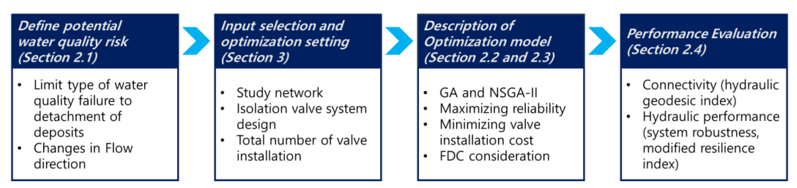
2. Methodology
2.1. Potential Water Quality Risks
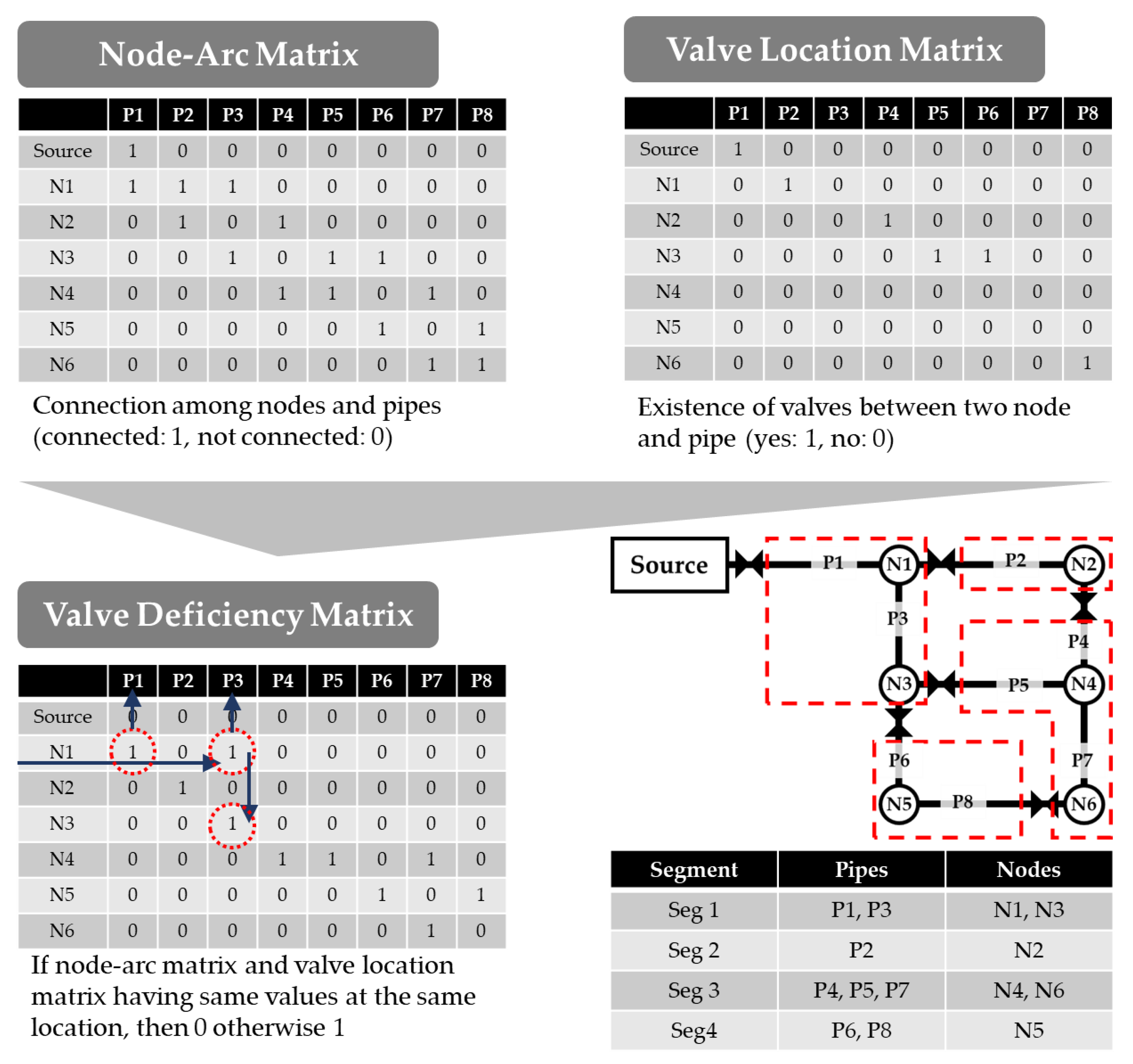
2.2. Segment Identification
2.3. Optimization Model
2.4. Performance Evaluation
2.4.1. Hydraulic Geodesic Index (HGI)
2.4.2. System Robustness Index (sysRob)
2.4.3. Modified Resilience Index (MRI)
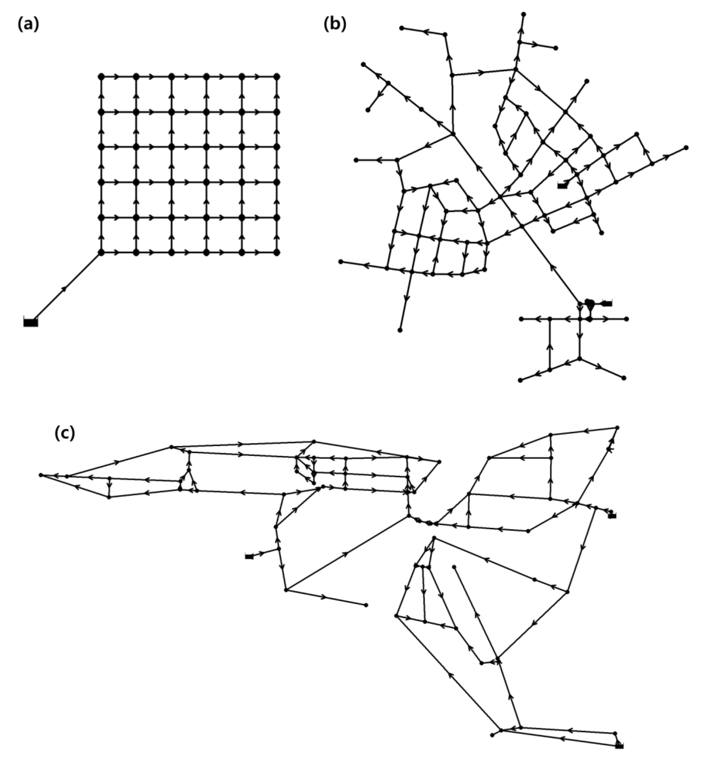
3. Study Networks
4. Application Results and Discussion
4.1. Optimization I
4.2. Optimization II
5. Conclusions
Author Contributions
Funding
Data Availability Statement
Conflicts of Interest
Abbreviations
| a ratio between 0 and 1.0 | |
| valve installation cost | |
| roughness coefficient of the i-th pipe | |
| diameter of the i-th pipe | |
| total number of flow direction change | |
| hydraulic geodesic | |
| hydraulic geodesic index | |
| represents the length of the i-th pipe | |
| the shortest value among all HG | |
| modified resilience index | |
| total number of segments | |
| number of valve installation | |
| total number of valves | |
| normalization | |
| normalized hydraulic geodesic index | |
| average of normalized hydraulic geodesic index | |
| total number of demand nodes | |
| number of pipes included in the segment | |
| PDA | pressure-driven analysis |
| average pressure of i-th node | |
| breakage probability for i-th pipe | |
| the probability of s-th segment isolation | |
| average reliability | |
| robustness of i-th node | |
| breakage rate per length (breaks/ft) for i-th pipe | |
| reliability during segment isolation | |
| system robustness | |
| actual demand (demand output of EPANET) | |
| required demand (base demand input of EPANET) | |
| weight of the i-th pipe | |
| the standard deviation of pressure at i-th node |
References
- Shin, S.; Lee, S.; Judi, D.R.; Parvania, M.; Goharian, E.; McPherson, T.; Burian, S.J. A Systematic Review of Quantitative Resilience Measures for Water Infrastructure Systems. Water 2018, 10, 164. [Google Scholar] [CrossRef]
- Lee, S.; Jung, D. Accounting for Phasing of Isolation Valve Installation in Water Distribution Networks. J. Water Resour. Plan. Manag. 2021, 147, 06021007. [Google Scholar] [CrossRef]
- Brentan, B.; Monteiro, L.; Carneiro, J.; Covas, D. Improving Water Age in Distribution Systems by Optimal Valve Operation. J. Water Resour. Plan. Manag. 2021, 147, 04021046. [Google Scholar] [CrossRef]
- Van Den Boomen, M.; Van Mazijk, A.; Beuken, R. First evaluation of new design concepts for self-cleaning distribution networks. J. Water Supply Res. Technol.—AQUA 2004, 53, 43–50. [Google Scholar] [CrossRef]
- Vreeburg JH, G.; Blokker, E.M.; Horst, P.; Van Dijk, J.C. Velocity-based self-cleaning residential drinking water distribution systems. Water Sci. Technol. Water Supply 2009, 9, 635–641. [Google Scholar] [CrossRef]
- Hong, S.; Lee, C.; Park, J.; Yoo, D.G. Velocity-based decision of water quality measurement locations for the identification of water quality problems in water supply systems. J. Korea Water Resour. Assoc. 2020, 53, 1015–1024. [Google Scholar]
- Walski, T.M. Valves and Water Distribution System Reliability; AWWA National Convention: New York, NY, USA, 1994. [Google Scholar]
- Jun, H.; Loganathan, G. Valve-controlled segments in water distribution systems. J. Water Resour. Plan. Manag. 2007, 133, 145–155. [Google Scholar] [CrossRef]
- Alvisi, S.; Creaco, E.; Franchini, M. Segment identification in water distribution systems. Urban Water J. 2011, 8, 203–217. [Google Scholar] [CrossRef]
- Giustolisi, O.; Savic, D. Identification of segments and optimal isolation valve system design in water distribution networks. Urban Water J. 2010, 7, 1–15. [Google Scholar] [CrossRef]
- Kao, J.-J.; Li, P.-H. A segment-based optimization model for water pipeline replacement. J. Am. Water Works Assoc. 2007, 99, 83–95. [Google Scholar] [CrossRef]
- Shuang, Q.; Liu, Y.; Tang, Y.; Liu, J.; Shuang, K. System reliability evaluation in water distribution networks with the impact of valves experiencing cascading failures. Water 2017, 9, 413. [Google Scholar] [CrossRef]
- Giustolisi, O. Water distribution network reliability assessment and isolation valve system. J. Water Resour. Plan. Manag. 2019, 146, 04019064. [Google Scholar] [CrossRef]
- Abdel-Mottaleb, N.; Walski, T. Evaluating segment and valve importance and vulnerability. J. Water Resour. Plan. Manag. 2021, 147, 04021020. [Google Scholar] [CrossRef]
- Wéber, R.; Huzsvár, T.; Hős, C. Isolation Valve Placement Optimization of Water Distribution Networks to Reduce Vulnerability. Period. Polytech. Mech. Eng. 2023, 67, 51–58. [Google Scholar] [CrossRef]
- Hernandez, E.; Ormsbee, L. Application of segment based robustness assessment for water distribution networks. In Proceedings of the International Joint Conference in Water Distribution Systems Analysis & Computing and Control in the Water Industry, Kingston, ON, Canada, 23–25 July 2018. [Google Scholar]
- Hernandez Hernandez, E.; Ormsbee, L. A Heuristic for Strategic Valve Placement. J. Water Resour. Plan. Manag. 2022, 148, 04021103. [Google Scholar] [CrossRef]
- Meng, F.; Sweetapple, C.; Fu, G. Placement of isolation valves for resilience management of water distribution systems. In Proceedings of the International Joint Conference in Water Distribution Systems Analysis & Computing and Control in the Water Industry, Kingston, ON, Canada, 23–25 July 2018. [Google Scholar]
- Yang, Z.; Guo, S.; Hu, Z.; Yao, D.; Wang, L.; Yang, B.; Liang, X. Optimal Placement of New Isolation Valves in a Water Distribution Network Considering Existing Valves. J. Water Resour. Plan. Manag. 2022, 148, 04022032. [Google Scholar] [CrossRef]
- Machell, J.; Boxall, J. Modeling and field work to investigate the relationship between age and quality of tap water. J. Water Resour. Plan. Manag. 2014, 140, 04014020. [Google Scholar] [CrossRef]
- Kang, D.; Lansey, K. Real-time optimal valve operation and booster disinfection for water quality in water distribution systems. J. Water Resour. Plan. Manag. 2009, 136, 463–473. [Google Scholar] [CrossRef]
- Dias, V.C.; Besner, M.-C.; Prevost, M. Predicting Water Quality Impact After District Metered Area Implementation in a Full-Scale Drinking Water Distribution System. J. AWWA 2017, 109, E363–E380. [Google Scholar] [CrossRef]
- Boxall, J.B.; Saul, A.J. Modeling Discoloration in Potable Water Distribution Systems. J. Environ. Eng. 2005, 131, 716–725. [Google Scholar] [CrossRef]
- Husband, S.; Boxall, J. Understanding and managing discolouration risk in trunk mains. Water Res. 2016, 107, 127–140. [Google Scholar] [CrossRef] [PubMed]
- Poulin, A.; Mailhot, A.; Periche, N.; Delorme, L.; Villeneuve, J.-P. Planning Unidirectional Flushing Operations as a Response to Drinking Water Distribution System Contamination. J. Water Resour. Plan. Manag. 2010, 136, 647–657. [Google Scholar] [CrossRef]
- Braga, A.S.; Saulnier, R.; Filion, Y.; Cushing, A. Dynamics of material detachment from drinking water pipes under flushing conditions in a full-scale drinking water laboratory system. Urban Water J. 2020, 17, 745–753. [Google Scholar] [CrossRef]
- Abraham, E.; Blokker, M.; Stoianov, I. Decreasing the Discoloration Risk of Drinking Water Distribution Systems through Optimized Topological Changes and Optimal Flow Velocity Control. J. Water Resour. Plan. Manag. 2018, 144, 878. [Google Scholar] [CrossRef]
- Armand, H.; Stoianov, I.; Graham, N. Investigating the Impact of Sectorized Networks on Discoloration. Procedia Eng. 2015, 119, 407–415. [Google Scholar] [CrossRef]
- Judi, D.R.; McPherson, T.N. Development of Extended Period Pressure-Dependent Demand Water Distribution Models; Los Alamos National Lab. (LANL): Los Alamos, NM, USA, 2015. [Google Scholar]
- Lee, S.; Jung, D. Shortest-Path-Based Two-Phase Design Model for Hydraulically Efficient Water Distribution Network: Preparing for Extreme Changes in Water Availability. IEEE Access 2021, 9, 53358–53369. [Google Scholar] [CrossRef]
- Jung, D.; Kang, D.; Kim, J.H.; Lansey, K. Robustness-Based Design of Water Distribution Systems. J. Water Resour. Plan. Manag. 2014, 140, 04014033. [Google Scholar] [CrossRef]
- Jayaram, N.; Srinivasan, K. Performance-based optimal design and rehabilitation of water distribution networks using life cycle costing. Water Resour. Res. 2008, 44, W01417. [Google Scholar] [CrossRef]
- Deuerlein, J.; Simpson, A.; Korth, A. Flushing Planner: A Tool for Planning and Optimization of Unidirectional Flushing. Procedia Eng. 2014, 70, 497–506. [Google Scholar] [CrossRef]
- Beuken, R. Validation New Design Rules for DWDS: Lab Experiments on Standard Sediment’; Report Number: BTO 2001.171; Kiwa WR NV: Nieuwegein, The Netherlands, 2001. [Google Scholar]
- Blokker, E.M.; Schaap, P.G.; Vreeburg, J.H. Comparing the fouling rate of a drinking water distribution system in two different configurations. In Proceedings of the 11th International Conference on Computing and Control for the Industry Urban Water Management, Exeter, UK, 5–7 September 2011; University of Exeter: Exeter, UK, 2011. [Google Scholar]
- Ahn, J.C.; Lee, S.W.; Choi, K.Y.; Koo, J.Y.; Jang, H.J. Application of unidirectional flushing in water distribution pipes. J. Water Supply Res. Technol.—AQUA 2011, 60, 40–50. [Google Scholar] [CrossRef]
- Armand, H.; Stoianov, I.I.; Graham, N.J.D. A holistic assessment of discolouration processes in water distribution networks. Urban Water J. 2015, 14, 263–277. [Google Scholar] [CrossRef]
- Creaco, E.; Haidar, H. Multiobjective Optimization of Control Valve Installation and DMA Creation for Reducing Leakage in Water Distribution Networks. J. Water Resour. Plan. Manag. 2019, 145, 04019046. [Google Scholar] [CrossRef]
- Su, Y.; Mays, L.W.; Duan, N.; Lansey, K.E. Reliability-Based Optimization Model for Water Distribution Systems. J. Hydraul. Eng. 1987, 113, 1539–1556. [Google Scholar] [CrossRef]
- Creaco, E.; Franchini, M.; Alvisi, S. Evaluating Water Demand Shortfalls in Segment Analysis. Water Resour. Manag. 2012, 26, 2301–2321. [Google Scholar] [CrossRef]
- Todini, E. Looped water distribution networks design using a resilience index based heuristic approach. Urban Water 2000, 2, 115–122. [Google Scholar] [CrossRef]
- Morosini, A.F.; Caruso, O.; Veltri, P. Management of water distribution systems in PDA conditions using isolation valves: Case studies of real networks. J. Hydroinform. 2019, 22, 681–690. [Google Scholar] [CrossRef]
- Islam, M.S. Water Distribution System Failures: An Integrated Framework for Prognostic and Diagnostic Analyses. Ph.D. Thesis, University of British Columbia, Vancouver, BC, Canada, 2012. [Google Scholar]
- Corso, P.S.; Kramer, M.H.; Blair, K.A.; Addiss, D.G.; Davis, J.P.; Haddix, A.C. Costs of illness in the 1993 waterborne Cryptosporidium outbreak, Milwaukee, Wisconsin. Emerg. Infect. Dis. 2003, 9, 426. [Google Scholar] [CrossRef]


| Optimization Model | Objective Function | Constraints |
|---|---|---|
| I | ||
| II |
| Scenario | RelAvg | FDC | norm SHGI | sysRob | Avg MRI | Avg Shortage | SD * Shortage |
|---|---|---|---|---|---|---|---|
| V30-1 | 0.893 | 0 | 0.859 | 0.579 | −0.375 | 480.26 | 825.16 |
| V30-2 | 0.898 | 42 | 0.857 | 0.550 | −0.565 | 480.26 | 819.71 |
| V40-1 | 0.925 | 0 | 0.918 | 0.688 | 0.035 | 280.15 | 663.17 |
| V40-2 | 0.931 | 46 | 0.915 | 0.675 | −0.037 | 281.66 | 660.18 |
| V50-1 | 0.942 | 0 | 0.945 | 0.745 | 0.224 | 186.69 | 562.53 |
| V50-2 | 0.950 | 46 | 0.940 | 0.702 | −0.042 | 198.08 | 563.31 |
| V60-1 | 0.948 | 0 | 0.957 | 0.763 | 0.262 | 146.78 | 532.75 |
| V60-2 | 0.961 | 56 | 0.952 | 0.744 | 0.146 | 150.43 | 518.29 |
| V70-1 | 0.953 | 0 | 0.966 | 0.780 | 0.314 | 115.29 | 501.07 |
| V70-2 | 0.967 | 70 | 0.963 | 0.777 | 0.271 | 116.37 | 459.81 |
| Scenario | NVal | CVal | RelAvg | FDC | norm SHGI | sysRob | Avg MRI | Avg Shortage | SD * Shortage | ||
|---|---|---|---|---|---|---|---|---|---|---|---|
| (1) | G | O | 93 | 144,069,465 | 0.956 | 0 | 0.971 | 0.834 | 0.315 | 100.38 | 482.29 |
| X | 93 | 144,069,465 | 0.970 | 50 | 0.968 | 0.773 | 0.294 | 102.35 | 471.44 | ||
| A | O | 60 | 949,219 | 0.870 | 0 | 0.897 | 0.328 | 0.094 | 551.88 | 1343.06 | |
| X | 65 | 943,002 | 0.928 | 86 | 0.925 | 0.692 | 0.091 | 398.24 | 1004.50 | ||
| P | O | 38 | 69,920 | 0.763 | 0 | 0.895 | 0.516 | −0.019 | 42.86 | 99.09 | |
| X | 39 | 69,718 | 0.919 | 158 | 0.891 | 0.586 | −0.039 | 43.44 | 57.75 | ||
| (2) | G | O | 93 | 144,069,465 | 0.956 | 0 | 0.971 | 0.834 | 0.315 | 100.38 | 482.29 |
| X | 62 | 96,046,310 | 0.956 | 44 | 0.943 | 0.726 | 0.307 | 187.09 | 546.52 | ||
| A | O | 60 | 949,219 | 0.870 | 0 | 0.897 | 0.328 | 0.094 | 551.88 | 1343.06 | |
| X | 63 | 634,926 | 0.880 | 46 | 0.909 | 0.276 | 0.093 | 474.48 | 1278.97 | ||
| P | O | 38 | 69,920 | 0.763 | 0 | 0.895 | 0.516 | −0.019 | 42.86 | 99.09 | |
| X | 29 | 46,324 | 0.819 | 52 | 0.858 | 0.409 | −0.030 | 60.72 | 70.10 | ||
Disclaimer/Publisher’s Note: The statements, opinions and data contained in all publications are solely those of the individual author(s) and contributor(s) and not of MDPI and/or the editor(s). MDPI and/or the editor(s) disclaim responsibility for any injury to people or property resulting from any ideas, methods, instructions or products referred to in the content. |
© 2023 by the authors. Licensee MDPI, Basel, Switzerland. This article is an open access article distributed under the terms and conditions of the Creative Commons Attribution (CC BY) license (https://creativecommons.org/licenses/by/4.0/).
Share and Cite
Shin, G.; Kwon, S.H.; Lee, S. Designing Isolation Valve System to Prevent Unexpected Water Quality Incident. Sustainability 2024, 16, 153. https://doi.org/10.3390/su16010153
Shin G, Kwon SH, Lee S. Designing Isolation Valve System to Prevent Unexpected Water Quality Incident. Sustainability. 2024; 16(1):153. https://doi.org/10.3390/su16010153
Chicago/Turabian StyleShin, Geumchae, Soon Ho Kwon, and Seungyub Lee. 2024. "Designing Isolation Valve System to Prevent Unexpected Water Quality Incident" Sustainability 16, no. 1: 153. https://doi.org/10.3390/su16010153
APA StyleShin, G., Kwon, S. H., & Lee, S. (2024). Designing Isolation Valve System to Prevent Unexpected Water Quality Incident. Sustainability, 16(1), 153. https://doi.org/10.3390/su16010153