Abstract
China’s sour gas reservoir is very rich in reserves, taking the largest whole offshore natural gas field in China-Puguang gas field as an example, its hydrogen sulfide content reaches 14.1%. The use of renewable energy, such as solar energy through photocatalytic technology, can decompose hydrogen sulfide into hydrogen and monomeric sulfur, thus realizing the conversion and resourceization of hydrogen sulfide gas, which has important research value. In this study, a concentration sample database of a hydrogen sulfide leakage scenario in a chemical park is constructed by Fluent software simulation, and then a leakage concentration prediction model is constructed based on the data samples to predict the hydrogen sulfide leakage diffusion concentration in real-time. Several machine learning algorithms, such as neural networks, support vector machines, and deep confidence networks, are implemented and compared to find the model algorithm with the best prediction performance. The prediction performance of the support vector machine model optimized by the sparrow search algorithm is found to be the best. The prediction model ensures the accuracy of the prediction results while greatly reducing the computational time cost, and the accuracy meets the requirements of practical engineering applications.
1. Introduction
As the use of chemicals continues to increase, leaks of hazardous chemicals [1] also occur frequently. Once such accidents occur, they can easily lead to serious consequences, such as property damage and casualties. Hydrogen sulfide [2] is often found in natural gas, which is a very important chemical raw material and is used in various fields, and there are many accidents caused by hydrogen sulfide leakage. On 12 July 2021, a hydrogen sulfide leak occurred at the Maidokawa Nuclear Power Plant in Miyagi Prefecture, Japan. The gas leaked from a storage tank in the waste treatment room of Unit 1 of the nuclear power plant and entered the adjacent Unit 2 control room through an air duct. Seven staff members in the control room suffered from varying degrees of poisoning after inhaling hydrogen sulfide. On 25 January 2021, a serious safety incident occurred at Sorik Marapi Geothermal Energy Ltd. in Indonesia during the commissioning of a power plant. When the geothermal well was opened, hydrogen sulfide gas [3] was released into the air, resulting in the death of five villagers from a nearby village and the hospitalization of nearly 20 villagers.
The accident analysis shows that incidents and accidents caused by poisoning by toxic and harmful gases of hydrogen sulfide have occurred repeatedly. Hydrogen sulfide is very dangerous in the production process, storage process, and transportation process and is prone to leakage accidents, and the lack of scientific research and evaluation of the spread of hydrogen sulfide leakage and the blind rescue of the rescuers at the scene will cause further expansion of the accident. It will also cause great difficulties for rescuers to organize a rescue. If the scope of hydrogen sulfide leak diffusion cannot be roughly calculated in advance, the personnel involved in the rescue will also be harmed, and once a leakage accident with serious consequences and great impact occurs, it will cause serious harm to people’s lives, properties, and the atmospheric environment. If the diffusion concentration of hydrogen sulfide leakage can be predicted in real-time, it can effectively help the emergency rescue team to determine the alert area and adjust the scope of the alert area in time to provide a technical guarantee for the emergency rescue work in the process of emergency rescue.
For the study of the method of toxic heavy gas leak diffusion prediction, mainly from the four aspects of experimental, theoretical, simulation, and statistical start, since the 1960s, some scholars have conducted many large-scale heavy gas release experiments. Table 1 lists a few typical experiments [4,5,6,7,8,9], with most of these experiments in the field open space because the heavy gas itself has a certain degree of danger. In addition, the field experiments have an experimental preparation workload and field experiments have the disadvantages of large experimental preparation, poor experimental reproducibility, and unpredictable experimental results.

Table 1.
Heavy gas release experiment.
To simplify the field experiments and make the operation of the experiments easier to control, researchers have found that the simulation of heavy gas diffusion can be carried out using laboratory simulation studies, such as wind tunnel tests and water tank experiments. As a result of its advantages of convenient field observation [10] and relatively simple operation, many experts have carried out wind tunnel simulation tests [11] with rich results, and European experts in heavy gas research have also established a set of wind tunnel test databases for researchers to analyze and study. However, the method cannot fully simulate the real leakage scenario, and the setting of the surrounding atmosphere and other conditions cannot be fully restored, so there is still a certain degree of error, and the reliability of the experimental results needs to be proven.
At the beginning of gas diffusion research, researchers believed that the gas followed a Gaussian distribution in the diffusion process, so the Gaussian diffusion model has been used for simulations of the diffusion of heavy gas [12]. However, with further scientific studies, researchers found that the Gaussian diffusion model [13] was more accurate in simulating the passive diffusion process of neutral and light gas clouds, and the results obtained in predicting the diffusion of simulated heavy gases differed greatly from the actual situation. Later, after decades of development and improvement, researchers established mathematical models applicable to the study of heavy gas diffusion simulations. In the 1970s, Blackmore and Wheatly [14,15] conducted a review and analysis of most of the heavy gas [16,17,18,19] diffusion models established at that time. The ones that are the most applied currently include the BM model [20], box model [21], shallow model [22], and hydrodynamic approach [23], but there are great limitations in the use of these models.
With the development of computer technology, numerical simulation and analysis methods have gradually become the main way to analyze the diffusion process of heavy gas. Hanna [24] used CFD models to numerically simulate the diffusion process of chlorine gas leakage in different scenarios, and their simulation results proved that CFD models simulate the local effects of building wake, slight terrain differences, and some mitigation measures (e.g., fencing). Pontiggia [25] used CFD tools to simulate the consequences of LPG railcar rupture in an urban area and found that obstacles have a significant impact on LPG dispersion in urban areas and that the real observed damaged areas are very similar to those predicted by CFD models. Dong [26] conducted a comprehensive field test of heavy gas leakage from a large building and simultaneously used four commonly used turbulence models for tests, which are important for the emergency response in the event of a leak in a large indoor space. Pan [27] used Fluent software to simulate the Thorney Island 026 experiment to observe the effect of obstacles on heavy gas diffusion and demonstrated that CFD simulates the heavy gas diffusion process in complex terrain. Gao [28] used Fluent software to simulate a natural gas pipeline leak to discuss the effect of wind speed on gas diffusion under different working conditions. This work can help emergency managers delineate the danger zone and evacuate people in time to ensure the smooth operation of emergency rescue work. However, to more realistically restore the situation when the gas leaks, the model grid needs to be finely divided, which makes the computer’s solution speed greatly reduced, and sometimes a large simulation project will take several days to receive the results of the simulation solution calculation, so it cannot track the prediction of heavy gas leakage accidents in real-time.
The advent of artificial intelligence has led to the integration of big data statistical methods into various disciplines, and this data-driven approach has led to the development of cross-disciplinary approaches and the rapid development of related theories that have brought unprecedented opportunities for the study of heavy gas leak prediction models. Some researchers have used artificial neural networks [29] or support vector machines [30] to predict the concentration change after a gas leak [31,32,33,34,35]. Kolehmainen [36] used an artificial neural network algorithm to computationally predict the urban air quality in Stockholm, and the results showed that the algorithm obtained fairly good predictions. Wang et al. [37] developed a fast method for predicting gas dispersion that collects data through gas detectors and then imports the data into an artificial neural network model for simulation, which allows bypassing difficult-to-obtain input parameters and using easily available parameters to predict gas dispersion concentrations for certain scenarios. Qiu et al. [38] proposed a new method for locating emission sources using artificial neural networks, particle swarms, and expectation maximization. A field study was conducted in Indianapolis to demonstrate that the method is feasible in practice, and the results of the field study show that the proposed method can estimate emission sources with acceptable accuracy and efficiency.
In this study, by analyzing the research history of heavy gas leak diffusion mentioned above, we found that researchers have conducted experiments and simulations for the situation after the accident. The existing gas diffusion concentration prediction models cannot combine accuracy and real-time, so there is a relative gap in the research on real-time prediction models for heavy gas leak diffusion concentrations. We consider the use of machine learning algorithms to develop a real-time prediction model for hydrogen sulfide leak dispersion concentration. Firstly, the CFD simulation software is used to simulate the hydrogen sulfide leakage dispersion process, and the data results obtained from the simulation are exported. After that, the data are processed and used as input samples for the machine algorithm model. Finally, the prediction models trained by machine learning are compared and evaluated to verify the accuracy and reliability of the models. The study will not only improve the safety level of the whole chemical park but also provide a richer, more intuitive, and more accurate decision-making basis for emergency rescue operations in case of accidents.
2. Numerical Simulation Analysis of Hydrogen Sulfide Leakage Dispersion Based on Fluent
2.1. Physical Model
The physical model of this study was selected from a part of a chemical enterprise park, which has three hydrogen sulfide storage tanks, several plants, two office buildings, and other production units. The simplified 3D physical model of the area was redrawn in Workbench’s DesignModeler software through the architectural 3D drawings provided by the enterprise, as shown in Figure 1.
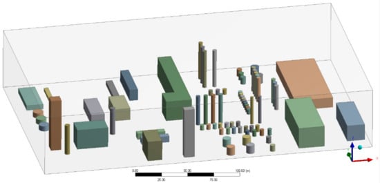
Figure 1.
Simplified physical model diagram.
When using CFD simulation calculation, a finite fluid domain is generally used instead of infinite space, so the model in this chapter, based on the actual size of the area in the CAD drawing and the approximate range of the gas after full diffusion, determines the size of the calculation area as a three-dimensional model with a length × width × height of 320 m × 200 m × 80 m, the leak source is located at the coordinate point (25, 100, 2.5), the leak height is 2500 mm, and the leak is a circular leak with a diameter of 300 mm.
2.2. Grid Division
Firstly, the overall mesh control is carried out using the system default tetrahedral unstructured mesh division, setting the physical field as CFD flow field, using the curvature function in the advanced dimension function, and setting the refinement mode of both the association center and the span center angle. Finally, the local cell size, contact area mesh setting, mesh shrinkage control, and expansion layer sets are then used to encrypt and refine the local mesh near the leakage port and the tank to improve the accuracy of the results. The final grid division results are shown in Figure 2, the total number of grids is 1,392,533, and then the grid quality was checked by using the grid measurement function. From Figure 3, it can be seen that the grid cell quality inspection and quadrilateral aspect ratio are very close to 1; skewness is close to 0; the maximum angle of the quadrilateral is close to 90°, which indicates that the established grid quality is good and can be used for subsequent simulation experiments.
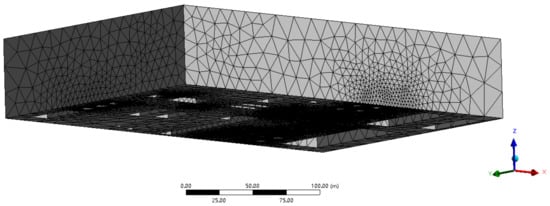
Figure 2.
Mesh division result.
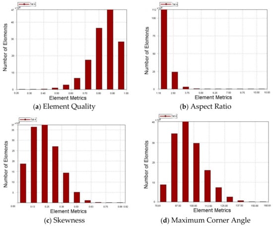
Figure 3.
Mesh quality check result.
2.3. Boundary Conditions
To begin, set the natural wind flowing from the x-axis negative direction to the x-axis positive direction, and then set the left side of the calculation domain as the wind speed inlet. However, different ground roughness in the boundary layer region needs to consider the viscous force, as the viscous force will have a great impact on the wind speed, and thus the wind speed will change with the height. This article uses an empirical formula (Equation (1)) to express the wind speed and uses UDF file programming to import its speed function; the tank leakage port is a mass inflow port; the ground and other obstacles are set as walls; the other faces of the fluid domain are set as pressure outlets.
where is the wind speed at the height at Z, is the meteorological forecast wind speed at distance from the ground, is the standard high speed at the wind observation point of the meteorological station, generally taken as 10 m, a is a constant, taking the value related to the roughness of the ground, generally flat and open countryside: a = 0.14; undulating hills: a = 0.28; downtown area: a = 0.4. Since the article simulates the leakage in the chemical park, a in the equation is taken as 0.4. When the wind speed observed by the weather station is 1.5 m/s, the curve of wind speed with the height is shown in Figure 4.
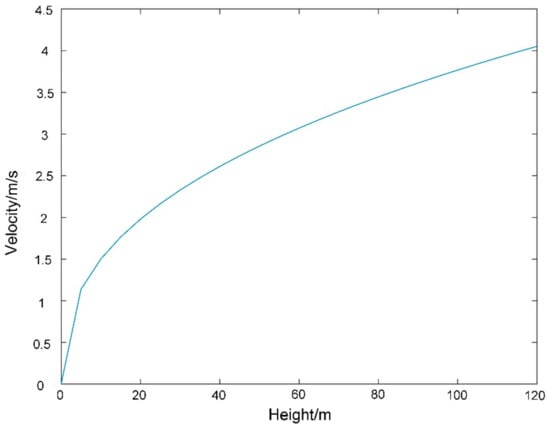
Figure 4.
The curve of wind speed versus altitude.
Since the concentration in the leakage area in the hydrogen sulfide leakage scenario is a dynamic process influenced by a variety of factors, this study mainly considers the initial state of the gas leakage, ground conditions, atmospheric stability, and other environmental parameters. The initial state of a gas leak contains the height of the leak source, the leak rate, and the direction of the leak, all of which have an impact on the concentration and trajectory of the heavy gas leak. First of all, the leak location may exist at the valve, flange connection, tank, and so on. Different leak locations will result in different leak rates, different angles of direction, and different concentrations of hazardous gases distribution. In addition, the larger the leak volume per unit of time, the larger the spread of the leak, the larger the danger area, and the greater the harm caused by the accident. The leak rate is related to the pressure inside the tank and the caliber of the leak. Ground conditions include the roughness of the ground and the number of obstacles, expressed in terms of the average height and density of the building complex. The greater the roughness of the ground, the less smooth the ground, and the less conducive to the diffusion of heavy gas. Atmospheric stability refers to the ability of the atmosphere to inhibit the vertical movement of air, and it has the most evident difference in the effect on the diffusion of heavy gases during the day and night. Daytime causes atmospheric instability due to sunlight temperature and other reasons, and the temperature difference between the surface and the atmosphere is large, which is conducive to the heat exchange of the gas, making its diffusion movement faster. At night the atmosphere is relatively stable, the opposite of the daytime situation, which is not conducive to the diffusion of heavy gases. Finally, there is the temperature. Generally, the higher the distance from the ground, the lower the temperature. When the temperature of the leaking heavy gas is higher than that of the surrounding air, it will lead to an enhanced tendency for the heavy gas to rise. When the temperature of the surrounding air is higher than the temperature of the leaking heavy gas, the stronger the energy exchange between the heavy gas and the surrounding air, the more likely the local turbulence phenomenon will be formed, and the degree of diffusion will increase. These nine input parameters as the subsequent prediction models are shown in Table 2. Wind speed, wind direction, and temperature are real-time data observed by weather stations when leakage occurs. The leak source height and leak velocity indicate the leak point, the azimuth angle indicates the direction of the leak, the distribution of buildings and structures is processed using the average height and density of the building complex, and finally, the Monin Obhof length is used to indicate the atmospheric stability.

Table 2.
Parameters for which data needs to be obtained.
In addition, all other boundary conditions are set as stationary non-slip walls with no return flow. According to the local weather station statistics, the variation interval of wind speed is set between 2–5 m/s, the temperature is selected between 0 °C and 25 °C, and the wind direction is selected between 0° (east wind) and 45° so that multiple sets of simulation calculations can be set up as a way to improve the diversity of samples.
2.4. Initialization
Import the meshed physical model into the Fluent module and perform the following initialization settings.
- 1.
- Set the 3D solver and non-stationary calculation, turn on the gravity option, and set the gravitational acceleration to extend the negative direction of the Z-axis with a magnitude of .
- 2.
- For the turbulence model, select the turbulence model and turn on the diffusion option.
- 3.
- The energy equation and component transport equation are opened, and the two-phase flow of hydrogen sulfide and air is set up in the gas mixture.
- 4.
- The PISO algorithm is chosen for the non-stationary calculation, followed by the initialization of the full space.
- 5.
- The step size is set to 0.2 s, with 1800 time steps and 10 iterations within each time step. Simulate the concentration distribution of hydrogen sulfide leakage for 5 min.
2.5. Simulation Results and Data Export
The Fluent simulation results were imported into Tecplot software for visual display. As a result of the large number of experimental results, only one group of experimental results images was selected for display. The wind speed of this group is set to 5 m/s, the temperature is 20 °C, the wind direction is 0°, and the leakage rate is 2 kg/s. The simulation results are shown in Figure 5.
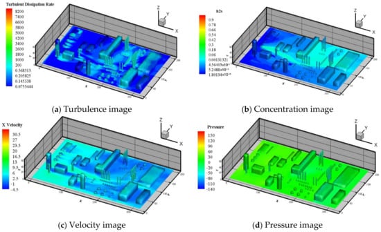
Figure 5.
Simulation results.
The results obtained from the simulation were further exported to the data by CFD-post post-processing software. To collect as much data as possible, a plane at a height of 2.5 m from the ground in the Z-axis direction was taken as the reference plane, and auxiliary lines were established in the X and Y directions from different orientation angles to export the temperature, velocity, and pressure data on the auxiliary lines for collation. Table 3 shows the derived data for some of the operating conditions, with the values of the leakage dispersion concentration at five-time points listed under each condition. One of the collected data sets is taken out as the test data set, and all the others are used as the training data set, thus making sufficient preparation for the subsequent machine learning model building.

Table 3.
Exported data for calculating the leakage concentration for partial conditions.
3. Machine Learning-Based Real-Time Prediction Model for Hydrogen Sulfide Leak Dispersion Concentration
3.1. Sample Data Pre-Processing
In this subsection, the bootstrapping method [39] is selected to divide the sample data. This method differs from stratified sampling methods such as cross-validation and leave-out methods in that it samples the data through a repeated sampling method with put-back. First, a sample is removed from the total data set and placed in the training set, and later put back, and the action of removing and putting back is repeated n times to obtain a training set of size n. The training set thus obtained must have duplicate samples and non-duplicate samples, after which the non-duplicate sample is used as the test set, and the probability that the sample will not be sampled is . The limit is taken as shown in Equation (2).
Therefore, 63.2% of the other total data were selected for the training data set, thus preventing pessimistic bias, and the remaining 36.8% of the data were used as the test set data.
By compiling and analyzing the sample data obtained from Table 2, it was learned that the data used to characterize the hydrogen sulfide concentration, such as wind speed, wind direction, and temperature, have very different magnitudes. The raw data are directly used in the model calculation, which will lead to a reduction in the efficiency of the model training and also have a great impact on the accuracy of the results. In addition, if the neural network model used subsequently has very large input values at the beginning of the training process, the applied weights must be very small to avoid saturation of the transfer function, and thus the gradient will become small. Therefore, the sample data need to be normalized before the model is trained, and the data are computationally mapped to the range of 0 to 1. The data normalization process is shown in Equation (3).
where and represent the values before and after normalization, respectively, and and represent the minimum and maximum values in the sample data, respectively.
3.2. Optimization Algorithm Performance Testing and Analysis
Since the value of the hyperparameters in the prediction model will affect the learning performance and effect of the model, optimization algorithms are often used to optimize the model to obtain a set of optimal hyperparameter values to improve the computing performance of the model. There are many kinds of existing optimization algorithms, and the standard test function can be used to test the performance of the optimization algorithms.
This section selects the multi-dimensional single-peak function, Sphere Function, the multi-dimensional multi-peak function, Rastrigin Function, and the fixed-dimensional (two-dimensional) multi-peak function, Schaffer Function, in the optimization class as the test functions to test the SA algorithm, GA algorithm, PSO algorithm, and SSA algorithm. Their definition domain, extreme value, and precision threshold are shown in Table 4.

Table 4.
Test functions.
The initial parameter selection of the four optimization algorithms follows the principle of fairness and sets them uniformly. The maximum number of iterations is set to 3000 times. The optimal solution of the function is set to zero. Each test function is independently repeated 30 times. The population size is set to 30. In addition, other initial parameters that have little influence on the experiment are kept at their default values. The results of the algorithm are recorded in the experiments for 30 runs of the extreme value calculation, and the optimal solution, the worst solution, the mean value, the mean square error, and the calculation time are calculated. The experimental results are provided in Table 5, Table 6 and Table 7. The average value and calculation time can reflect the convergence speed of the algorithm, and the mean square error can reflect the stability of the algorithm.

Table 5.
Experimental results of 10-dimensional Sphere function and Rastrigin function.

Table 6.
Experimental results of 20-dimensional Sphere function and Rastrigin function.

Table 7.
Experimental results of fixed dimension (two-dimensional) Schaffer function.
Table 5 and Table 6 show the performance test results of the algorithms in the 10- and 20-dimensional cases, respectively. The results of all four algorithms are accurate when dealing with 10-dimensional functions. However, in terms of computational speed, the annealing algorithm and genetic algorithm compute more slowly than the other two algorithms. When the dimension of the test function is increased to 20 dimensions, all four algorithms do not perform well in handling the Rastrigin test function, and the annealing algorithm and the particle swarm algorithm even fall into the local optimum. It can also be seen that the stability of the convergence of the algorithms decreases as the dimensionality increases, which means that there are shortcomings in using these algorithms to solve high-dimensional problems. Combining the convergence curves of the four algorithms to observe the experimental results of the multidimensional multi-peak test function, the particle swarm algorithm and the sparrow search algorithm take the least computational time and converge the fastest, both converging within 500 iterations, while the annealing algorithm and the genetic algorithm require more than 1000 iterations to converge.
Table 7 shows the experimental results in a fixed dimension (two dimensions). From the data in the table, it can be seen that both the particle swarm algorithm and the sparrow search algorithm find the optimal solution of the Schaffer test function with two-dimensional multiple peaks, and the stability of the algorithm during the solution is similar, but the sparrow search algorithm takes the least time to compute. Thus, the performance of the Sparrow search algorithm in solving the Schaffer test function is better than the other three algorithms in terms of the optimal solution, the worst solution, the mean value, the mean squared error, and the time spent. After comprehensive consideration, it was decided to use the sparrow search algorithm for the optimization calculation of the hyperparameter selection for the subsequent model.
3.3. Establish a Real-Time Prediction Model for Hydrogen Sulfide Leakage Diffusion Concentration
There is a wide variety of prediction models, each with different characteristics. It is necessary to conduct experiments to compare and analyze how to select the best model algorithm that is most applicable to the object to be studied. The accuracy and generalization ability of each model’s computational results is discussed comprehensively through experiments to select the optimal model. In this paper, three models, BP neural network, support vector machine, and deep confidence network, are selected to compare the real-time prediction of hydrogen sulfide leakage, and the model calculation process is designed as shown in Figure 6.
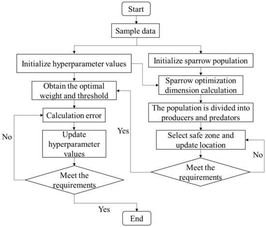
Figure 6.
The sparrow search algorithm optimizes the prediction model process.
Finally, the pre-processed dataset is imported into three machine learning prediction models optimized by the sparrow search algorithm, and the model prediction results are compared and analyzed. The experimental environment configurations involved in the paper for relevant model building, validation, and comparison are shown in Table 8.

Table 8.
Configuration and environment.
4. Model Evaluation and Results
4.1. Fluent Model Validation
Due to the special nature of hydrogen sulfide heavy gas, it is not feasible to conduct field gas concentration dispersion experiments, and thus difficult to verify its CFD simulation results for field experiments. How to verify the accuracy of CFD simulation results has also been an important factor hindering the development of simulation software. Inspired by the conference on drag prediction, Zhang [40] introduced the concept of CFD uncertainty and proposed a validation method in addition to the field experimental results verification. By performing several simulations using different meshes and different formats and afterward using the law of large numbers to calculate their mathematical expectations for comparative validation. This also allows the accuracy of the simulation results to be verified.
The real value is assumed to be R, and the simulated calculated value is . The concept of uncertainty was first introduced to describe the difference between the real and calculated values in terms of the maximum of the absolute values.
The meaning of CFD uncertainty, as proposed by Zhang, is that the calculated value of the simulation can reach the first n digits of the real value, i.e.,
where η is required to satisfy the following conditions:
To determine the first n bits of the true value, it is necessary to establish a data band and to ensure that all data in the data band satisfy the first n bits of the true value accurately. The prerequisite for the establishment of the data band is to ensure that this quantity can be calculated using multiple computational methods to obtain its computational results and that the CFD simulation results satisfy its condition. Multiple calculations can be performed for the simulated scenario using different grid numbers and different turbulence calculation models. Table 9 shows the results of the concentration calculations using the standard model and the realizable model for the same leak moment under six different sets of grid numbers.

Table 9.
Calculation results of two turbulence models with different meshes.
The law of large numbers and the statistical calculation method are introduced here. Assuming that the discrete data of the calculation results obtained by each different calculation method are , and in addition is the probability of their occurrence, the weighted average is:
Generally speaking, the more the number of grids, the more accurate the simulation results. Firstly, the number of grids is taken as the weight, and the number of grids is brought into Equation (7). After that, let and the predicted true value can be obtained as follows.
In turn, the bits of data that are close to the true value are determined, and finally, their error values are calculated as follows.
The above steps were calculated to obtain the data close to the real value by a few digits and to obtain the optimal solution and the error value. With these two parameter values, it is possible to go through the evaluation of the accuracy of the simulation results. The optimal solution result values and error values are given in Table 10. It can be seen that the optimal value is quite close to the real value, thus proving the accuracy of the simulation results.

Table 10.
Comparison results between optimal solution and true value.
4.2. Predictive Model Performance Evaluation
Since three different algorithmic models are used to train the sample data in this paper, the same rubric needs to be used to verify the model’s performance. Therefore, the root mean square error and the correlation coefficient are used uniformly to evaluate the model performance. The smaller the RMSE value, the smaller the prediction error value of the model. The closer the correlation coefficient is to 1, the better the model fit is. The formulas for calculating the root mean square error and correlation coefficient are shown below.
where n is the number of samples in the test set, , is the predicted value of the i-th sample data, and is the calculated value of the i-th sample.
In this paper, the true and predicted value results of the test set of the obtained experimental results are plotted as images, and the comparison of the true and predicted values of the experimental results of the test set of the three prediction models obtained is shown in Figure 7, Figure 8 and Figure 9. By observing the calculation results of the models, it can be seen that the SSA-DBN model has the best prediction results. Its RMSE value is 0.000405, which is very close to 0, and the R2 value is 0.98631, which is very close to 1. The SSA-SVM model results are not very different from it, and the simulation results are also relatively good. Only the SSA-BP model has a large difference in the resulting error compared with the other two prediction models, and the performance of the model is relatively poor.
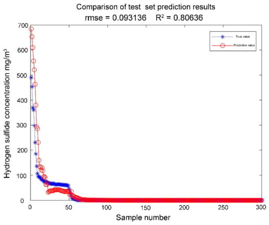
Figure 7.
SSA-BP model calculation results.
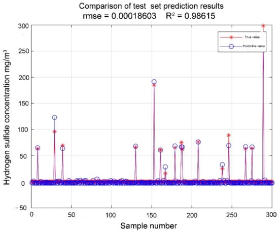
Figure 8.
SSA-SVM model calculation results.
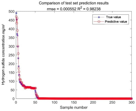
Figure 9.
SSA-DBN model calculation results.
Figure 10 shows the convergence process of the algorithm model, and the gradient of the adaptive function in the sparrow search algorithm is gradually decreasing as the number of iterations increases, indicating that the SSA algorithm plays a good optimization role. The final results of using the sparrow search algorithm to optimize the hyperparameters in all three models are smoothly converged. During the parameter optimization process of the SSA-BP model, the fitness value of the function decreases in a step-like manner, and it finally converges after the number of iterations reaches about 200 times. In the process of optimizing the parameters of the SSA-SVM model, the fitness value of the function dropped sharply at the beginning of the calculation, and it became stable after iterating to 80 generations. With the increase in the number of iterations, the fitness value basically does not change, indicating that the sparrow search algorithm finds the hyperparameters C and g of the support vector machine model faster. In the parameter search process of the SSA-DBN model, there is a significant decrease in the function fitness value at the beginning, but it tends to level off again in the middle section. There is another significant decrease at 130 generations, and finally, it converges at about 150 generations, and the convergence speed is slower compared to the other two prediction models. In addition, the comparison of the fitness values shows that SSA-SVM has the smallest fitness value, which indicates that the model fits better during the training process compared to the other two models.
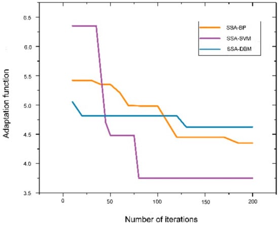
Figure 10.
Convergence curve.
In order to ensure the rigor of the experimental calculations of the three hydrogen sulfide leak diffusion concentration prediction models optimized by the sparrow search algorithm, the unoptimized BP, SVM, and DBN models, i.e., the empirical models, were used to predict the hydrogen sulfide leak concentration for comparison. The results are shown in Table 11, where the accuracy of the optimized prediction results is substantially improved, and the time spent on calculation is not significantly increased. It is obvious that the performance of the prediction model is better after the optimization of the sparrow search algorithm.

Table 11.
Prediction effect of each model.
Since there is a certain randomness in the simple cross-validation, in order to compare the performance of the three models more fairly, each model is operated 10 times independently, and its mean value is taken before comparison. The comparison results are shown in Table 11 and Figure 11, from which it can be seen that the support vector machine prediction model optimized by the sparrow search algorithm performs better than the other two models. The accuracy of the BP neural network model is not satisfactory because of its low function approximation and generalization ability. It is further verified that the SSA-SVM model has superior accuracy for hydrogen sulfide leak diffusion concentration prediction.
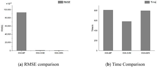
Figure 11.
Model effect comparison.
New technologies emerging from the field of big data will make data-driven class models play a greater role. While traditional gas leak dispersion models cannot combine real-time prediction with accuracy, the machine learning models established in this study all have a prediction time of less than one second and higher accuracy than traditional prediction models. In practical engineering applications, the models established by using this study can directly calculate real-time data monitored by field detectors and weather stations as samples, thus ensuring real-time and accurate prediction results.
5. Conclusions
Once the toxic heavy gas leaks, it will not only cause casualties and property losses but also the air pollution it causes seriously restricts the sustainable development of the environment. In this paper, based on a systematic review of heavy gas leak diffusion concentration research, a real-time prediction model of hydrogen sulfide leak diffusion concentration based on a machine learning algorithm is proposed, and the method is validated by taking a chemical park as an example. We use Fluent simulation software to study the influencing factors affecting hydrogen sulfide leak dispersion and train the simulation results as the sample data for the prediction model. The accuracy of the computational results and the excellent model performance were compared between traditional neural networks, integrated learning, and deep learning, and the superiority of the performance of the support vector machine model optimized by the sparrow search algorithm was demonstrated. The experimental results show that our model can be used for real-time prediction of diffusion concentration of hydrogen sulfide gas leakage in chemical parks, and the accuracy of its prediction results can meet the requirements of practical engineering applications. It not only has a certain guiding significance for the emergency rescue operations after the leakage of hydrogen sulfide gas in chemical parks but also has a certain reference significance for the planning and design of safety development in chemical parks. In addition, in terms of prediction time, the prediction of hydrogen sulfide leak diffusion concentration using the machine algorithm model is less than 1 s. It can be seen that the machine learning algorithm greatly reduces the computational time cost while ensuring the accuracy of the prediction results.
Related studies have demonstrated that heavy gas leak dispersion can be simulated using computational fluid dynamics simulation software, and heavy gas leak dispersion can be predicted using artificial intelligence algorithms. This study not only demonstrates the feasibility of these methods but also proposes a more novel approach to predict the diffusion concentration of hydrogen sulfide leaks in real-time. Despite the innovative nature of the methods used in this study, there are some shortcomings (1) for the applicability of the model. Although the model can be extended to other cases of heavy gas leakage, it is only applicable to point source leakage of the gas in a particular scenario. If it is applied to other scenarios, it is still necessary to re-collect data and organize the data samples to retrain the model. (2) The amount of sample data required for training machine learning algorithms is huge, which plays a key role in the success of the prediction model. However, existing data on heavy gas leaks such as hydrogen sulfide are scarce and difficult to obtain, so this paper uses CFD software to perform accurate numerical simulations and uses the data results obtained from the simulations as samples for modeling. Although the prediction time is significantly saved, the cost of collecting data upfront is too large in order to reproduce the real situation of leakage.
Author Contributions
Methodology, X.T.; software, X.T.; validation, X.T., D.W., S.W. and X.P.; formal analysis, X.T.; investigation, D.W.; resources, D.W.; data curation, X.T.; writing—original draft preparation, D.W.; writing—review and editing, X.T.; project administration, X.T. and X.P. All authors have read and agreed to the published version of the manuscript.
Funding
This research received no external funding.
Data Availability Statement
The data used to support the findings of this study are included within the article.
Conflicts of Interest
The authors declared no potential conflict of interest with respect to the research, authorship, and/or publication of this article.
References
- Wu, M.; Zhang, G.; Zhang, G.W.; An, Z.Y.; Liu, X. Modelling of hazardous chemical gas building ingress and consequence analysis during a leak accident. Indoor Built Environ. 2023, 32, 1420326X221137244. [Google Scholar] [CrossRef]
- Omagari, S.; Taniguchi, N.; Yokogawa, Y.; Yoneda, M.; Yamamoto, S.; Hanioka, T.; Hirofuji, T. Inhibitory Mechanisms of S-PRG Eluate and S-PRG Filler against Volatilization of Hydrogen Sulfide. Oper. Dent. Endodontology Periodontol. 2021, 1, 30–36. [Google Scholar]
- Niu, W.; Kang, K.; Ou, Y.; Ding, Y.; Du, B.; Guo, X.; Tan, Y.; Hu, W.; Gao, C.; He, Y.; et al. Cobalt ions induced morphology control of metal-organic framework-derived indium oxide nanostructures for high performance hydrogen sulfide gas sensors. Sens. Actuators B Chem. 2023, 381, 133347. [Google Scholar] [CrossRef]
- Ma, D.; Gao, J.; Zhang, Z.; Zhao, H. Identifying atmospheric pollutant sources using a machine learning dispersion model and Markov chain Monte Carlo methods. Stoch. Environ. Res. Risk Assess. 2021, 35, 271–286. [Google Scholar] [CrossRef]
- Maithili, S.; Pramod, K. An analytical model for crosswind integrated concentrations released from a continuous source in a finite atmospheric boundary layer. Atmos. Environ. 2009, 43, 2268–2277. [Google Scholar]
- Carvalho, J.D.C.; Degrazia, G.A.; Anfossi, D.; De Campos, C.R.J.; Roberti, D.R.; Kerr, A.S. Lagrangian stochastic dispersion modelling for the simulation of the release of contaminants from tall and low sources. Meteorol. Z. 2002, 11, 89–97. [Google Scholar] [CrossRef]
- Pramod, K.; Maithili, S. An analytical model for dispersion of pollutants from a continuous source in the atmospheric boundary layer. Proc. R. Soc. A Math. Phys. Eng. Sci. 2010, 466, 406–466. [Google Scholar]
- Qian, W.; Venkatram, A. Performance of Steady-State Dispersion Models Under Low Wind-Speed Conditions. Bound. Layer Meteorol. 2011, 138, 475–491. [Google Scholar] [CrossRef]
- Britter, R.E.; Hanna, S.R.; Briggs, G.A.; Robins, A. Short-range vertical dispersion from a ground level source in a turbulent boundary layer. Atmos. Environ. 2003, 37, 3885–3894. [Google Scholar] [CrossRef]
- Li, S.; Li, X.; Li, J.; Su, Y.; Wu, B. Measurements of the unsteady lift force on a 5,1 rectangular cylinder based on active-passive hybrid wind tunnel tests. Measurement 2023, 213, 112674. [Google Scholar] [CrossRef]
- Li, Y.; Sun, P.P.; Li, A.; Deng, Y. Wind Effect Analysis of a High-rise Ancient Wooden Tower with a Particular Architectural Profile via Wind Tunnel Test. Int. J. Archit. Herit. 2023, 17, 518–537. [Google Scholar] [CrossRef]
- Miller, C.W.; Hively, L.M. A review of validation studies for the Gaussian plume atmospheric dispersion model. Nucl. Saf. 1987, 28, 522–531. [Google Scholar]
- Yizhe, L.; Qi, Y. Combined Grey Wolf Optimizer Algorithm and Corrected Gaussian Diffusion Model in Source Term Estimation. Processes 2022, 10, 1238. [Google Scholar]
- Blackmore, D.R.; Herman, M.N.; Woodward, J.L. Heavy gas dispersion models. J. Hazard. Mater. 1982, 6, 107–128. [Google Scholar] [CrossRef]
- Wheatley, C.J.; Webber, D.M. Aspects of the Dispersion of Denser-Than-Air Vapours Relevant to Gas Cloud-Explosions; Springer: Dordrecht, The Netherlands, 1985; pp. 191–200. [Google Scholar]
- Ahuja, V.; Bhatt, A.K.; Ravindran, B.; Yang, Y.-H.; Bhatia, S.K. A Mini-Review on Syngas Fermentation to Bio-Alcohols: Current Status and Challenges. Sustainability 2023, 15, 3765. [Google Scholar] [CrossRef]
- Quiralte, D.; Zarzo, I.; Fernandez-Zamudio, M.-A.; Barco, H.; Soriano, J.M. Urban Honey: A Review of Its Physical, Chemical, and Biological Parameters That Connect It to the Environment. Sustainability 2023, 15, 2764. [Google Scholar] [CrossRef]
- Liang, Z.; Luo, Z.; Yuan, J.; Li, M.; Xia, Y.; Che, T.; Huang, L.; Liu, J. Evaluating the Environmental and Economic Performance of Municipal Solid Waste Disposal by All-Component Resource Recovery. Sustainability 2022, 14, 16898. [Google Scholar] [CrossRef]
- Livaniou, S.; Papadopoulos, G.A. Liquefied Natural Gas (LNG) as a Transitional Choice Replacing Marine Conventional Fuels (Heavy Fuel Oil/Marine Diesel Oil), towards the Era of Decarbonisation. Sustainability 2022, 14, 16364. [Google Scholar] [CrossRef]
- Jin, J.L.; Jin, B.M.; Ding, J. A nonlinear time-series model for predicting atmospheric CO2 concentration. J. Nat. Disasters 2000, 4, 76–79. [Google Scholar]
- Zeman, O. The dynamics and modeling of heavier-than-air, cold gas release. Atmos. Environ. 1982, 16, 741–751. [Google Scholar] [CrossRef]
- Robin, K.; Hankin, S. Heavy gas dispersion: Integral models and shallow layer models. J. Hazard. Mater. 2003, 103, 1–10. [Google Scholar]
- Li, X.; Zhou, N.; Chen, B.; Zhang, Q.; Rasouli, V.; Liu, X.; Huang, W.; Kong, L. Numerical Simulation of Leakage and Diffusion Process of LNG Storage Tanks. Energies 2021, 14, 6282. [Google Scholar] [CrossRef]
- Hanna, S.R.; Hansen, O.R.; Ichard, M.; Strimaitis, D. CFD model simulation of dispersion from chlorine railcar releases in industrial and urban areas. Atmos. Environ. 2009, 43, 262–270. [Google Scholar] [CrossRef]
- Pontiggia, M.; Landucci, G.; Busini, V.; Derudi, M.; Alba, M.; Scaioni, M.; Bonvicini, S.; Cozzani, V.; Rota, R. CFD model simulation of LPG dispersion in urban areas. Atmos. Environ. 2011, 45, 3913–3923. [Google Scholar] [CrossRef]
- Dong, L.; Zuo, H.; Hu, L.; Yang, B.; Li, L.; Wu, L. Simulation of heavy gas dispersion in a large indoor space. using CFD model. J. Loss Prev. Process Ind. 2017, 46, 1–12. [Google Scholar] [CrossRef]
- Wu, Y.J.; Pan, X.H. CFD simulation validation of heavy gas leakage dispersion experiments under obstacle terrain conditions. J. Saf. Sci. Technol. 2010, 6, 13–17. [Google Scholar]
- Gao, L.J.; Wu, M.M. Numerical Simulation of Leak Dispersion in Overhead Sulfur-Containing Natural Gas Pipelines. China Water Transp. 2016, 2, 31–33. [Google Scholar]
- Baker, T.; Hammerstrom, D. Characterization of artificial neural network algorithms. In Proceedings of the IEEE International Symposium on Circuits and Systems, Portland, OR, USA, 8–11 May 1989; pp. 78–81. [Google Scholar]
- Noble, W.S. What is a support vector machine? Nat. Biotechnol. 2006, 24, 1565–1567. [Google Scholar] [CrossRef]
- Tian, X.; Jiao, W.; Liu, T.; Ren, L.; Song, B. Leakage detection of low-pressure gas distribution pipeline system based on linear fitting and extreme learning machine. Int. J. Press. Vessel. Pip. 2021, 194, 104553. [Google Scholar] [CrossRef]
- Sinha, S.; de Lima, R.P.; Lin, Y.; Sun, A.Y.; Symons, N.; Pawar, R.; Guthrie, G. Normal or abnormal? Machine learning for the leakage detection in carbon sequestration projects using pressure field data. Int. J. Greenh. Gas Control 2020, 103, 103189. [Google Scholar] [CrossRef]
- Da Cruz, R.P.; da Silva, F.V.; Fileti, A.M.F. Machine learning and acoustic method applied to leak detection and location in low-pressure gas pipelines. Clean Techn. Environ. Policy 2020, 22, 627–638. [Google Scholar] [CrossRef]
- Iwaszenko, S.; Kalisz, P.; Słota, M.; Rudzki, A. Detection of Natural Gas Leakages Using a Laser-Based Methane Sensor and UAV. Remote Sens. 2021, 13, 510. [Google Scholar] [CrossRef]
- NK, B.; Sasmal, S.; Voggu, S. Machine learning supported acoustic emission technique for leakage detection in pipelines. Int. J. Press. Vessel. Pip. 2020, 188, 104243. [Google Scholar]
- Kolehmainen, M.; Martikainen, H.; Ruuskanen, J. Neural networks a and periodic components used in air quality forecasting. Atmos. Environ. 2001, 35, 815–8250. [Google Scholar] [CrossRef]
- Wang, B.; Chen, B.; Zhao, J. The real-time estimation of hazardous gas dispersion by the integration of gas detectors, neural network and gas dispersion models. J. Hazard. Mater. 2015, 300, 433–442. [Google Scholar] [CrossRef]
- Qiu, S.; Chen, B.; Wang, R.; Zhu, Z.; Wang, Y.; Qiu, X. Atmospheric dispersion prediction and source estimation of hazardous gas using artificial neural network, particle swarm optimization and expectation maximization. Atmos. Environ. 2018, 178, 158–163. [Google Scholar] [CrossRef]
- Freund, Y.; Schapire, R.E. A decision-theoretic generalization of on-line learning and an application to boosting. J. Comput. Syst. Sci. 1997, 55, 119–139. [Google Scholar] [CrossRef]
- Zhang, H.X. Numerical simulation study on CFD with high accuracy and fidelity. Acta Aerodyn. Sin. 2016, 34, 1–4. [Google Scholar]
Disclaimer/Publisher’s Note: The statements, opinions and data contained in all publications are solely those of the individual author(s) and contributor(s) and not of MDPI and/or the editor(s). MDPI and/or the editor(s) disclaim responsibility for any injury to people or property resulting from any ideas, methods, instructions or products referred to in the content. |
© 2023 by the authors. Licensee MDPI, Basel, Switzerland. This article is an open access article distributed under the terms and conditions of the Creative Commons Attribution (CC BY) license (https://creativecommons.org/licenses/by/4.0/).