1. Introduction
A number of factors (energy crisis, wars, climate change, etc.) are causing a rise in renewable energies use. Solar energy can be easily and affordably converted either into thermal energy by means of thermal panels or into electrical energy, using photovoltaic panels (PV) [
1]. Industrial plants generating electricity from solar energy, commonly known as solar farms, are generally composed of a high number of photovoltaic (PV) panels made of PV cells. As the number of installations increases, the maintenance of solar farms becomes a nontrivial problem [
2]. The energy produced depends on different conditions, such as the state of the panels, the climate, or the time of year. Solar panels are also vulnerable to phenomena that can reduce or nullify their performance. These issues make necessary a system to control and optimize production, since manual human labor is not enough as the number of panels gets higher.
Artificial intelligence is usually applied to solve difficult control and optimization problems. When applied to PV systems, different AI methods such as fuzzy logic, metaheuristics, or neural networks have been used to solve problems [
3]. The most important problems include [
4] max power point tracking, output power forecasting, parameter estimation, and defect detection.
Defect detection is one of the most interesting problems and researched topics in PV systems [
5,
6]. It is usually tackled with different kinds of neural networks, since they have great performance, although, as an important drawback, they need high amounts of data to perform better than other machine learning methods [
7]. This could be a major impossibility for problems where it is difficult to harvest new data. Most of the approaches to detect the state of PV panels use electroluminescence images of the cells as an input, which is an invasive method that makes it difficult to carry out measurements and gather data.
Data augmentation is the most common method to deal with image data scarcity by means of the introduction of slight modifications (rotations, flips, and minor deformations) to the original images in order to create new images [
8,
9,
10]. More recent papers promote the use of more complex AI techniques, such as Generative Adversarial Networks (GANs), to generate synthetic images [
11,
12]. GANs are state-of-the-art algorithms for data generation [
13]. They have also been applied to PV systems for solving different problems [
14].
The generation of synthetic EL images of PV cells using GANs has also been proposed in other works [
11,
12]. These works present synthetic datasets created with different GAN architectures trained with EL images of cells with different kinds of defects. Although the datasets in these works have not been made public, from their work, it can be deduced that the synthetic images are just labeled from visual inspection in order to train standard defect/normal classifiers, ignoring the output energy output performance of synthetic cells, since they cannot be measured.
In this paper, we present a new approach to deal with the image data scarcity problem. Starting from a small set of electroluminescence images of PV cells obtained under experimental conditions to be described, a synthetic dataset of images was created using Generative Adversarial Networks (GANs). For each synthetic image, a scalar value that represents the performance of their energy production is associated using machine learning techniques trained with the energy production of the original PV cells. It is also a continuation of the paper presented in [
15], where we augmented and improved the dataset and applied new metrics to ensure the appropriate quality of the generated data.
To ensure reproducibility, the resulting dataset was made publicly available, so it can be used to improve the performance of AI models, to analyze the characteristics, properties, and defects of the cells, or to compare with other methods of generation of synthetic images.
This paper is structured as follows:
Section 2 briefly reviews the Generative Adversarial Networks,
Section 3 presents the methodology that was followed to generate the dataset, in
Section 4, the synthetic dataset is described, and finally, the conclusions of the paper are presented in
Section 5.
2. Generative Adversarial Networks
Generative Adversarial Networks (GANs) [
16] are one of the most important and popular technologies nowadays and have been applied to different fields [
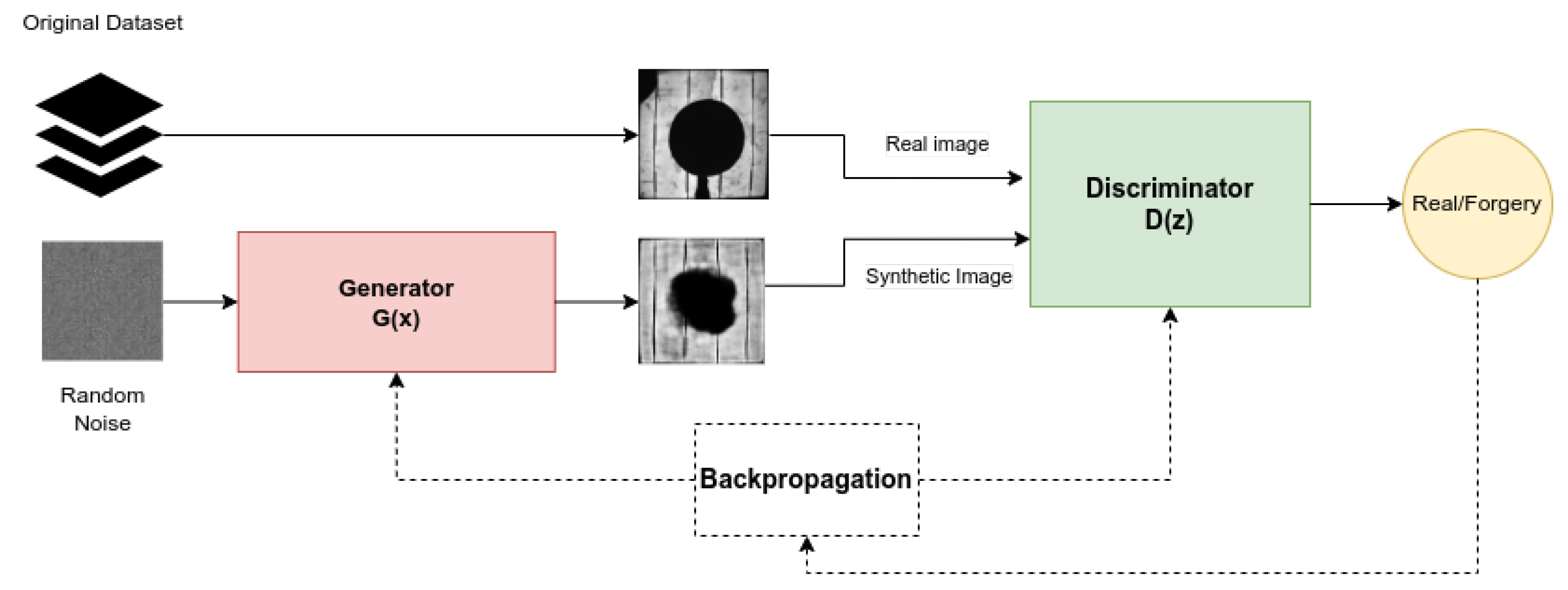
17]. They can be applied to semisupervised and unsupervised learning. A GAN is usually defined as a pair of neural networks that are competing against each other. The network known as the Generator is the one designed with the job of trying realistic new data to try to deceive the other network, known as the Discriminator. This network has to decide if the data that it receives were forged.
The Generator does not have access to the real data, which is an important feature of these algorithms. The Generator has to learn how to create the data based on the feedback from the Discriminator. The Discriminator has access to both kinds of data, but it does not know which kind of data is an image before carrying out the prediction. The networks change their weights depending on the results of the deception; the Generator uses them to improve the forgeries, while the Discriminator tries to improve its recognition of forgeries.
Figure 1 shows a diagram of the behavior of the algorithm.
The basic principle of operation of a GAN can be expressed as a two-player minimax game played between D and G, with a value function
given by the following mathematical expression [
16], a binary cross-entropy function, commonly used in binary classification problems:
The first term in (
1) represents the expected value of entropy given by the Discriminator over the real data and the second is the entropy given by the Generator over the fake data obtained.
GANs are usually composed of Deep Feed-forward Networks, but more complex architectures can be used in order to improve the generative capacities of the algorithm and the quality of the forged data. One of the most used architectures are Convolutional Neural Networks.
Deep Convolutional GAN
Research on GANs has led to new interesting architectures which substantially improve the performance of the networks and the quality of the forged data [
18]. For this paper, we implemented the architecture known as Deep Convolutional GAN [
19]. This architecture is based on convolutional layers, but it also provides a set of constraints in order to provide more stabilized training and better quality in the output. The most important guidelines are the following:
Use of batch normalization in the Generator and the Discriminator.
Removal of fully connected hidden layers in both networks.
Usage of convolutional transposed layers instead of the stridden convolutional layers. This is only applied in the Generator network.
3. Methodology
The correct preparation of the real and synthetic image datasets is a complex process which requires several steps to complete. In this section, we present the methodology that was followed in this research, which implies four relevant stages: manual acquisition of real EL images of PV cells beside their electrical characteristics (IV curves); data preprocessing to prepare for synthetic image generation using GAN; maximum power output assignment to synthetic cells from regression models trained with real images; and model and result validation.
3.1. Real Images Acquisition
Data availability is one of the most critical issues when using deep learning techniques. For precise PV cell characterization, we need two different kinds of data: the electroluminescence (EL) images of the photovoltaic cells and their corresponding IV curves. For the first, there are some public datasets available in the bibliography [
20], but they do not include information about the IV curve, since it is not easy to measure the individual curve of a single PV cell. To solve this problem, we had to obtain the data using a specific technique developed previously [
21] and following a manual process in the laboratory.
The capturing of the EL images was performed using a Hamamatsu InGaAs Camera C12741-03. The cell was isolated from external light in other to avoid the light produced by other kinds of radiations.
Figure 2a presents the camera for taking the pictures. EL was chosen as the image capture technique, since it is widely used for detecting defects on PV modules [
22] and it is the most used technique in other related works with PV systems. In order to test the different levels of luminous emission of the cell, various values of current were used to power the LED array when obtaining the IV curve and to the PV cell when capturing the EL image.
To measure the IV curve, we used a device specifically designed to measure the values of current and voltage of a single cell [
21]. This device (
Figure 2b) provided voltage and current values to build the IV curve of the cells. The IV curves can be used to calculate the max power point and the performance of the cells.
Figure 2c shows the setting used for taking the IV curves. The original paper for this device validates the accuracy of the measurements.
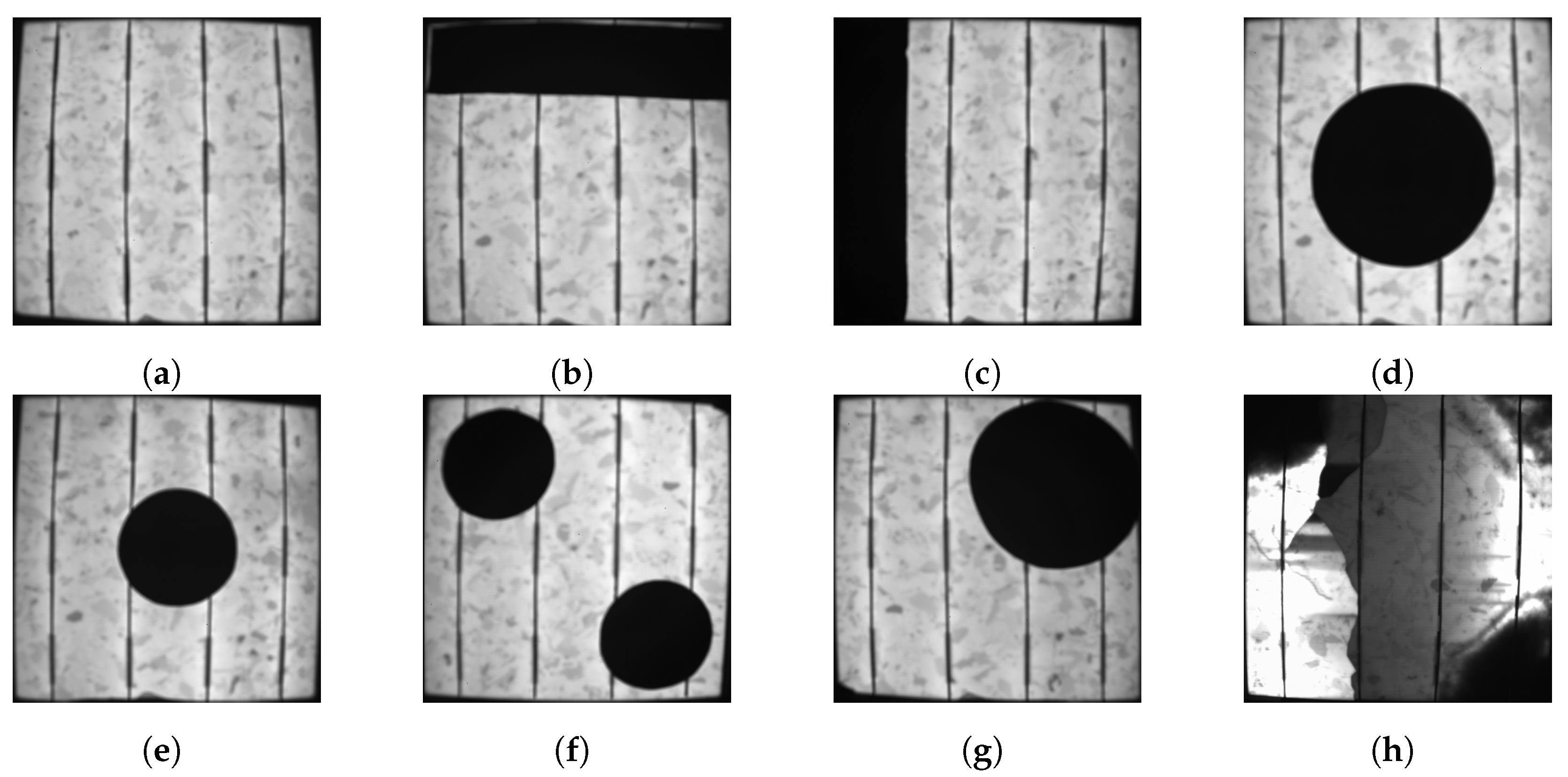
The number of damaged cells was extremely limited in quantity and variety. The solution for this issue was to create artificial shadows in order to improve the amount and variety of images. The different shadows were created taking into account the most important defects found in solar farms.
Figure 3 presents a representative image of each kind of artificial shadow that was used.
The final acquired dataset was composed of 602 different EL images with their corresponding IV curves. In order to allow the repeatability of the experiments, the dataset was made publicly available (The dataset can be downloaded from
https://github.com/hectorfelipe98/Synthetic-PV-cell-dataset. The repository includes the original images, the synthetic dataset, and a CSV file that maps each image with its relative power and its class).
3.2. Image Preprocessing
The captured EL images were not suitable to be directly used with machine learning algorithms, since there were factors affecting image quality to be addressed first. For this reason, some algorithms were used to improve both the quality and normalization of the images. This section explains how the different problems found in image quality were solved.
Dead pixels and luminous noise: The insulation of the system when capturing the images was not perfect. Some leaks could be found in some cases. This produced luminous noise when the image was taken. Another problem could be found in the camera. Due to its extended use, the camera had some dead pixels. Even though these phenomena are not easily visible to the human eye, they degenerate the quality of the obtained images. In order to solve these two problems, an image was taken before the real measure and without turning on the lights from the LED array. This provided information about the luminous noise and the dead pixel of the camera. Having this information, it is possible to perform a subtraction of the noise from the original image. This process was performed for each of the EL images.
Images with poor lighting: The scale of the histograms of the images can produce problems in some libraries or programs which cannot recognize which values correspond with the white color.
Figure 4a,b shows how the values are distributed in only a small fraction of the possible values, which makes the image look extremely dark. The solution to this problem corresponds to performing a min–max normalization, subtracting the minimum values of the image, and dividing it by the maximum value. The resulting image can be found in
Figure 4c,d.
Figure 4.
Image before and after applying color normalization: (a) original image; (b) original histogram; (c) image after the min–max normalization; and (d) histogram after the normalization.
Figure 4.
Image before and after applying color normalization: (a) original image; (b) original histogram; (c) image after the min–max normalization; and (d) histogram after the normalization.
Black surrounding contours:
Figure 4c shows how images are surrounded by a black area. The reason for this phenomenon is caused by a limited focusing of the camera, which is capturing part of the walls of the insulated area. The solution to this issue consisted of performing a change in perspective. The first step consisted of applying different filters in order to delete the details, obtaining the maximum contour polygon of the cell. The next step consisted of performing a Hough transform to find the corners of the cells, using the polygon calculated previously as the base. In some cells, it was necessary to make some tweaks manually, as they presented strange defects that notably changed the aspect of the cell. The results of the transformation can be found in
Figure 5.
3.3. Generation of the Synthetic Images
As announced, a Deep Convolutional Generative Adversarial Network was chosen to generate extra images from the original recorded set. The model is composed of two different networks: the Generator and the Discriminator. This section explains the architecture and parameters of both networks and the process of training.
3.3.1. Generative Network
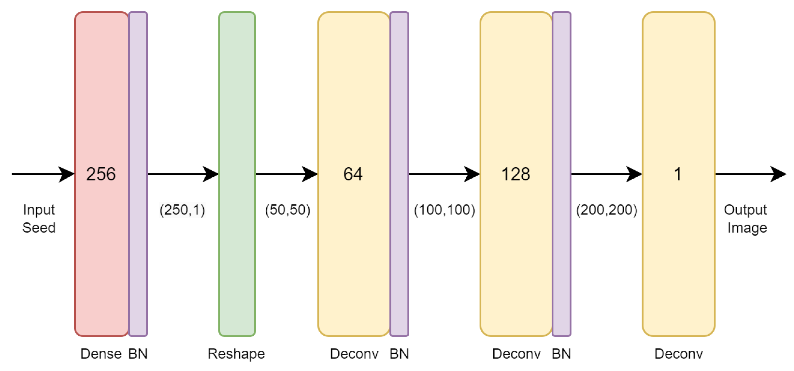
The generative network was created following the principles of the DCGN. It has 3 different Convolutional Transpose Layers (Deconvolutional) in order to generate patterns. The use of these layers in combination with batch normalization [
23] improves the generative capacities of the network and improves the stability of the training, The network uses Leaky Relu [
24] as an activation function, since it usually outperforms the standard Relu. The architecture of this networks is represented in
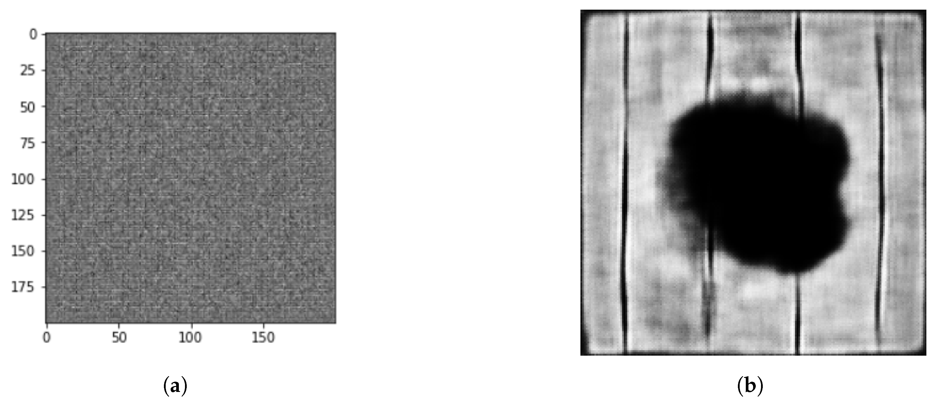
Figure 6. The input to the network (
Figure 7a) is a random noise array from a normal distribution. The output is a 200 × 200 image (
Figure 7b. This size was chosen in order to reduce the computation cost of the algorithm while still obtaining images with a large amount of information. Other important hyperparameters can be found in
Table 1.
3.3.2. Discriminator Network
The Discriminator network also followed the principles of DCGAN. The network uses different Convolutional Neural Networks to find patterns from the images. The typical feed-forward part of the network was also removed, with only the output layer remaining. The use of dropout layers and batch normalization improves the generalization capacity of the networks and stabilizes the training. The architecture is represented in
Figure 8. The input corresponds to a 200 × 200 image and the output to a binary value that determines if the image is a real cell or a forgery. The other important hyperparameters were the same as the Generator, so they can be found in
Table 1.
3.3.3. Training the GAN
The training was performed simultaneously in both networks with all the available samples (602). The training loop starts with the creation of synthetic images by the Generator using random seeds. After that, the Discriminator is provided with a mix of real and synthetic images. That input data are used to train the network, the loss is computed for each of the networks, based on the results of the Discriminator.
Figure 9 shows the evolution of the loss for both networks. In the first epochs, the loss of the Discriminator network is quite high. It has not learned the patterns of the original images, so it cannot identify which images are real or forgered, even if the forged images are extremely similar to noise. After a while, the Discriminator reduces its loss since it can differentiate which images are real; this provokes an increase in the loss of the Generator. After that, the loss of the Generator steadily decreases its value since it starts to learn the patterns to create images similar to the original ones. Until epoch 400, it continues to learn when it obtains its lowest value. At the same time, the Discriminator is unable to identify which images are real, making its loss its maximum value. After epoch 400, the values have almost no change, so it can be concluded that the training should end at this point.
The training was performed with a CPU AMD Ryzen 7 5800H, 16 GB of RAM, and a GPU Nvidia Geforce GTX 1650. It took 2 h and 41 min to complete the training.
After completing the training, the Generator network was used to generate the synthetic dataset. A total of 10,000 different images were created using 10,000 different random seeds.
Figure 10 presents a selection of some generated images.
3.4. Assigning Maximum Power to Cells
The labeling of the images was not a trivial process, since it required associating each image (real or synthetic) with an output maximum power value, which represents the performance of the cell. This section explains how this association was made both for original and GAN-generated images.
3.4.1. Original Images
As explained before, each EL image has an associated IV curve. The IV curve provides information about the performance of the cell, which can only be obtained after taking the following steps:
Compute the power–voltage curve of each cell from its IV curve.
The maximum value of the curve is saved as the max power point (MPP).
We gather the cells into 6 groups, in terms of the irradiance used to excite the cell before emission, since the MPP depends on the amount of light projected onto the cell.
For each group, the 5 highest values of MPP are considered, and their mean is calculated.
This average of the maximum values is understood as the expected MPP of a cell without any defects or shadows in that group.
The MPP of each cell is divided by the averge MPP of the cell group it belongs to.
The resulting value will measure the relative performance of the cell, normalizing its MPP with the maximum value of the cells of the same group. This maximum is the mean of the 5 highest values, since it reduces the effects of potential incorrect measurement. Values of relative power near 1 will correspond with cells in good condition, with only a few or no defects. Low values correspond with underperforming cells, mostly due to their defects.
3.4.2. Synthetic Images
The labeling of the synthetic dataset was a completely different problem. As explained, the values of the original images were calculated based on their IV curve. This process cannot be replicated in the synthetic images, since they are not real cells; so, they cannot be measured.
To solve this problem, we formulated it as a regression problem that can be solved using a machine learning model. The model is trained with the full dataset of original images, together with their normalized power (MPP) calculated from IV curves, as explained in the previous subsection (602 samples). The chosen model is Random Forest [
25], since it provided a low error in the original dataset and showed excellent generalization power to associate the MPP to the synthetic images. The implementation of the algorithm in the Sklearn library [
26] was used for this work. The tuning of the hyperparameters of the RF model was carried out using the Grid Search method in the Sklearn library (GridSearchCV), obtaining the optimal values shown in
Table 2.
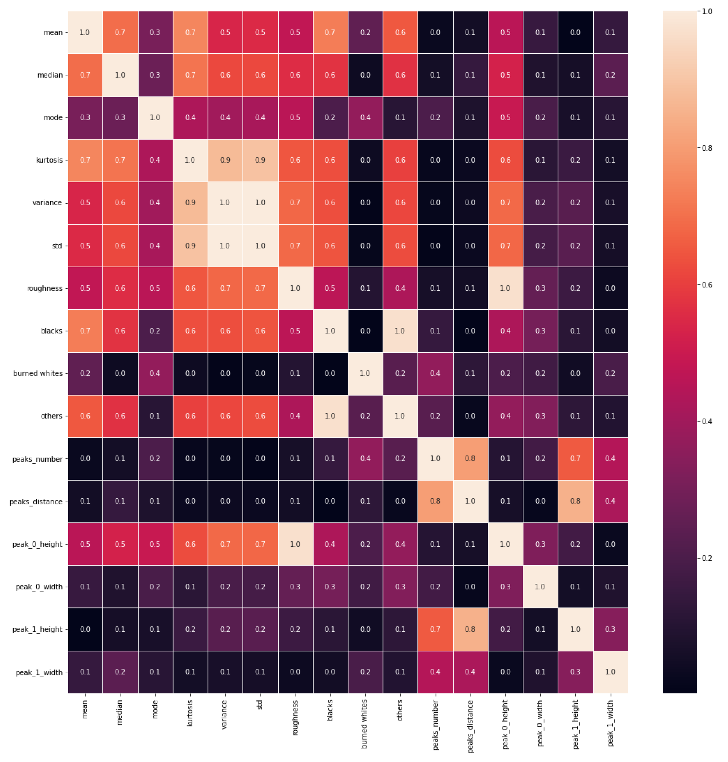
Since Random Forest is not suitable to work directly on raw images, some features were extracted from the images. The features are based on typical statistics (mean, standard deviation, etc.) and other characteristics directly extracted from the histogram (amounts peaks, peaks width, peaks height, amount of colors, etc.) A complete list can be found in
Table 3. Feature selection (FS) is an important step in the preparation of machine learning models. We used correlation-based FS. As depicted in
Figure 11, the cross-correlation between all the original sets of features shows that almost no feature is highly correlated with the others, except for the standard deviation and the variance, which are completely dependent on each other, meaning one of them can thus be safely removed from the final set of features.
The dataset was split into two sets: training (67%) and validation (33%). We decided to only use two due to our data limitation. The target variable was the relative power of each cell, standardized between 0 and 1.
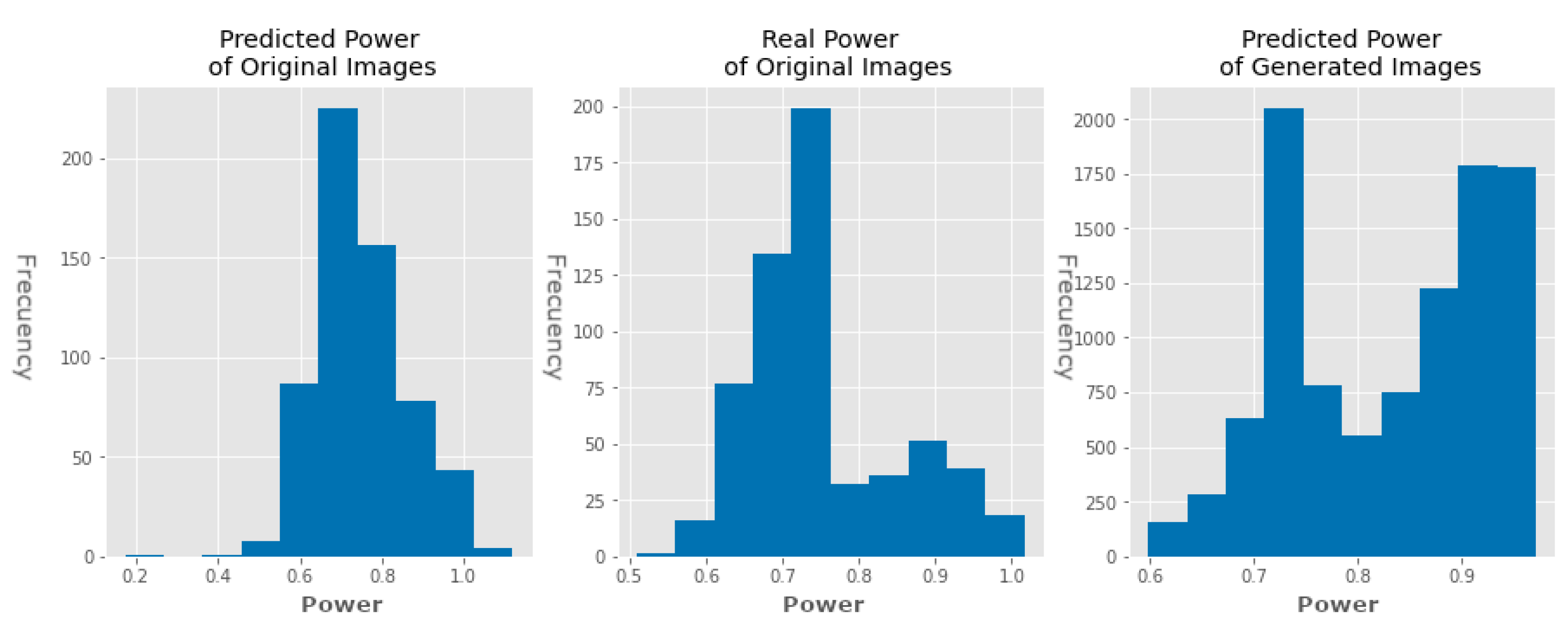
The model obtained a Mean Absolute Error (MAE) of 0.041 and a Mean Squared Error (MSE) of 0.0038 in the validation dataset. The distribution of the predictions of the model can be found in
Figure 12. The low error and the similarity in the distribution confirm the validity of the model. The distribution of the prediction for the synthetic dataset can also be observed. Finally, the images were divided into two groups according to their predicted power (class 0
and class 1
). In total, 6963 images were classified as class 0 and 3037 as class 1.
4. Results
The resulting dataset was divided into two different folders, one for each class: Class 0 (6963 samples,
Figure 13a) represented the images whose relative power is at least 0.8, and the images in that class can be considered as functional PV cells. Class 1 (3037 samples,
Figure 13b) represented the images with a power of less than 0.8, and the images in that class can be considered as underperforming PV cells.
4.1. Visual Analysis
For ensuring the quality and similarity of the images, we propose two different methods: in this section, an analysis based on visual characteristics and histogram, and in the next section, an analysis based on different metrics.
As can be observed in
Figure 13, the generated images present a similar structure while presenting new patterns of shadows different from the original ones (
Figure 3). This is an interesting feature produced by the generative capacity of the GAN, since it can combine the different kinds of shadows presented in the original images in order to create new kinds of patterns. This improves the variety of shadows presented in the dataset.
Figure 14 presents the distribution of the features selected previously for labeling (
Table 3). For each feature, the relationship between the values of the feature and the relative power of the cell is presented. Synthetic images are represented with orange dots, and the original images are represented with blue dots. In most features, the original dataset images appear as a subset of the synthetic dataset, with some exceptions caused mostly by underrepresented cases. This means that synthetic images not only present the characteristics of the original images, but they also present new cases of defects or shadows while maintaining the most important characteristics. This is mostly produced by the generative properties of the GAN, which can create new patterns combining the patterns of the input data; these new patterns improve the diversity of the dataset. This can lead to an improvement in performance in the machine learning methods that use this dataset. Another interesting finding is that the most underrepresented cases in the original data do not appear in the synthetic data; this is also provoked by the properties of the GAN, since it needs a considerable amount of samples to find patterns.
4.2. Histogram Analysis
The histogram of the images gives a lot of information about them.
Figure 15a presents the mean histogram of all images of class 0 of the original dataset and the mean for all of the pictures of class 0 of the synthetic one. It can be seen that the images in this class present a large amount of light gray–white pixels (Values near 200), but they also can present some minor defects or shadows, as can be seen by the number of black pixels (values near 0). A difference between both datasets can be seen: the synthetic dataset images have higher but narrower peaks and are sometimes a bit moved to the left.
Figure 15a presents the same information for the images in class 1. The images in this class present a large number of dark pixels due to their defects and shadows. The amount of lighter pixels is considerably lower. In the synthetic images, the peak of black pixels is higher, but its width is narrower. The light pixels are extremely similar to the original ones.
As shown, the aspect of the histograms of both datasets is quite similar. The minor differences are mostly produced due to the augmented variety of patterns of defects and shadows.
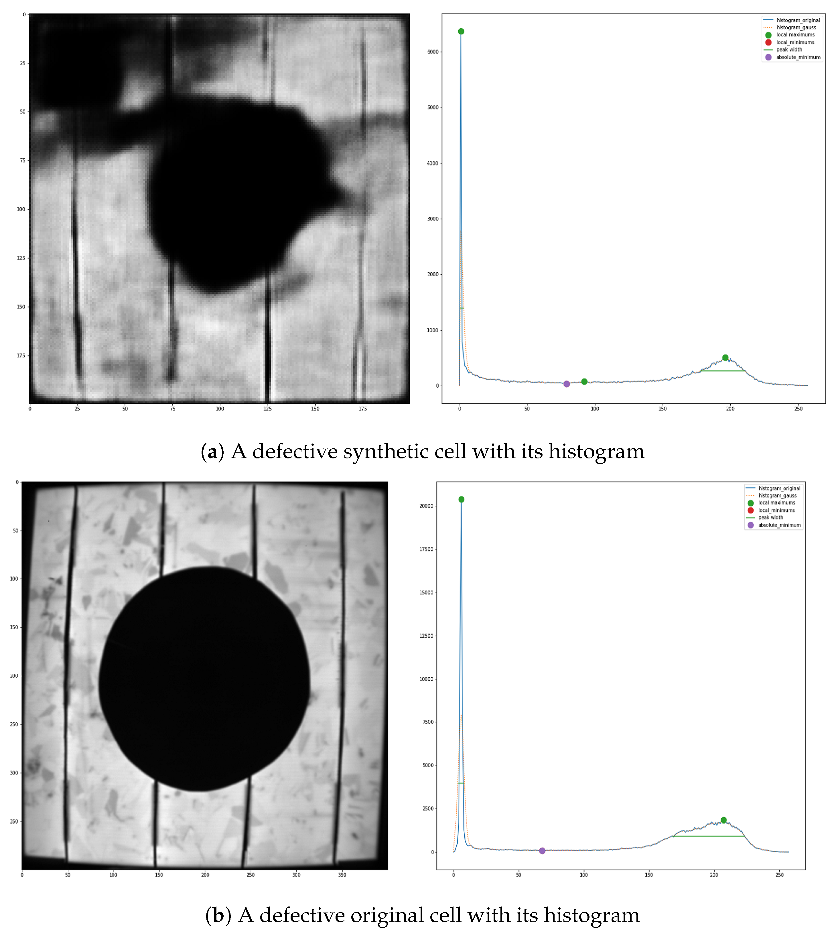
Figure 16 presents two different cells of class 1: one original and one synthetic with similar aspects. Visual inspection of both histograms shows that they have a similar structure, presenting the same amount of peaks and even placed in a similar position. Nevertheless, synthetic images tend to show a more symmetrical histogram and a shift from maximum to lower intensities, since the extreme intensity values are less frequent than in real images.
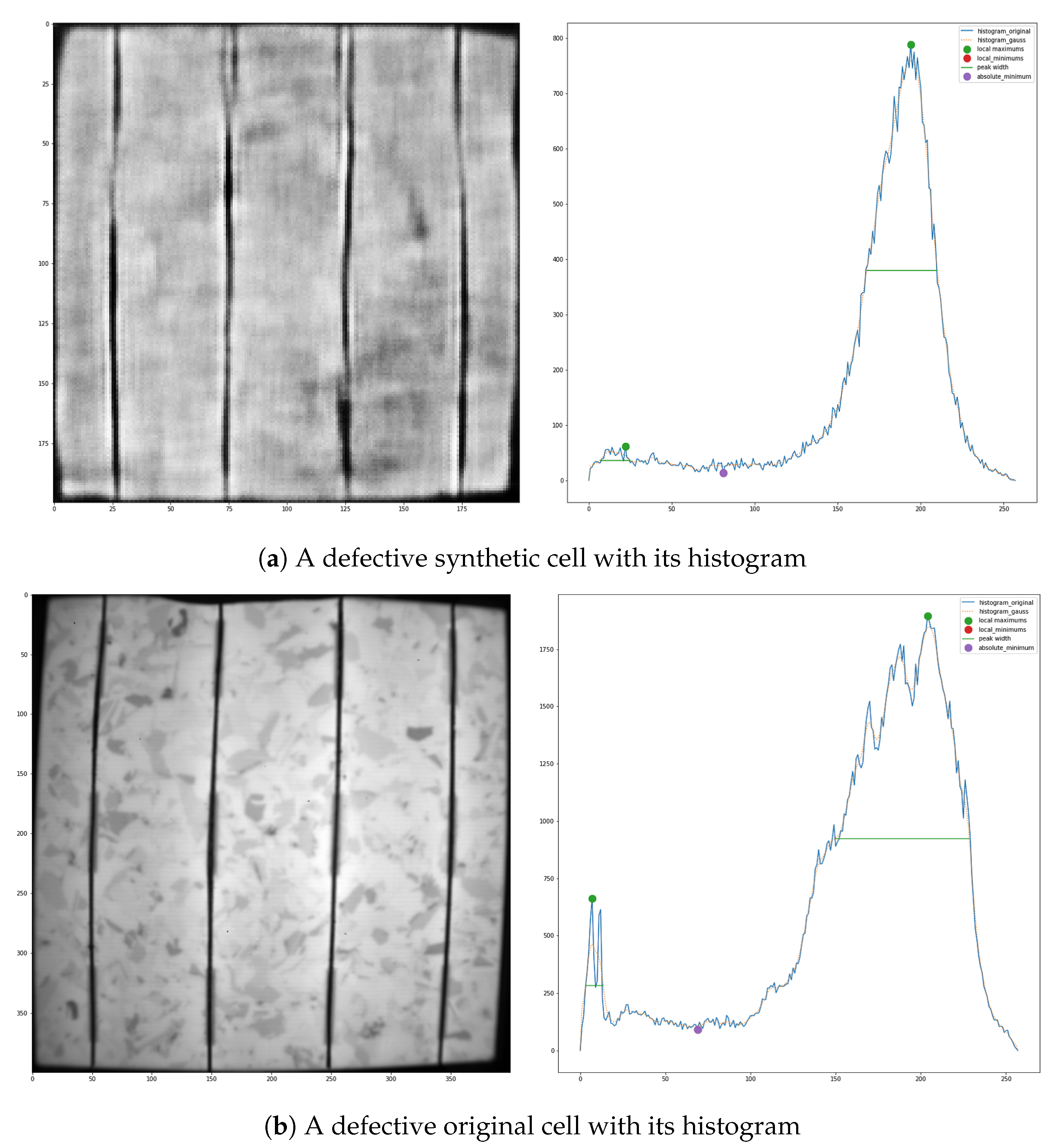
Figure 17 presents the same for two images of class 0. Both images have almost no apparent defects. Their histograms have similar shapes, as can be seen by the number of peaks and their placement.
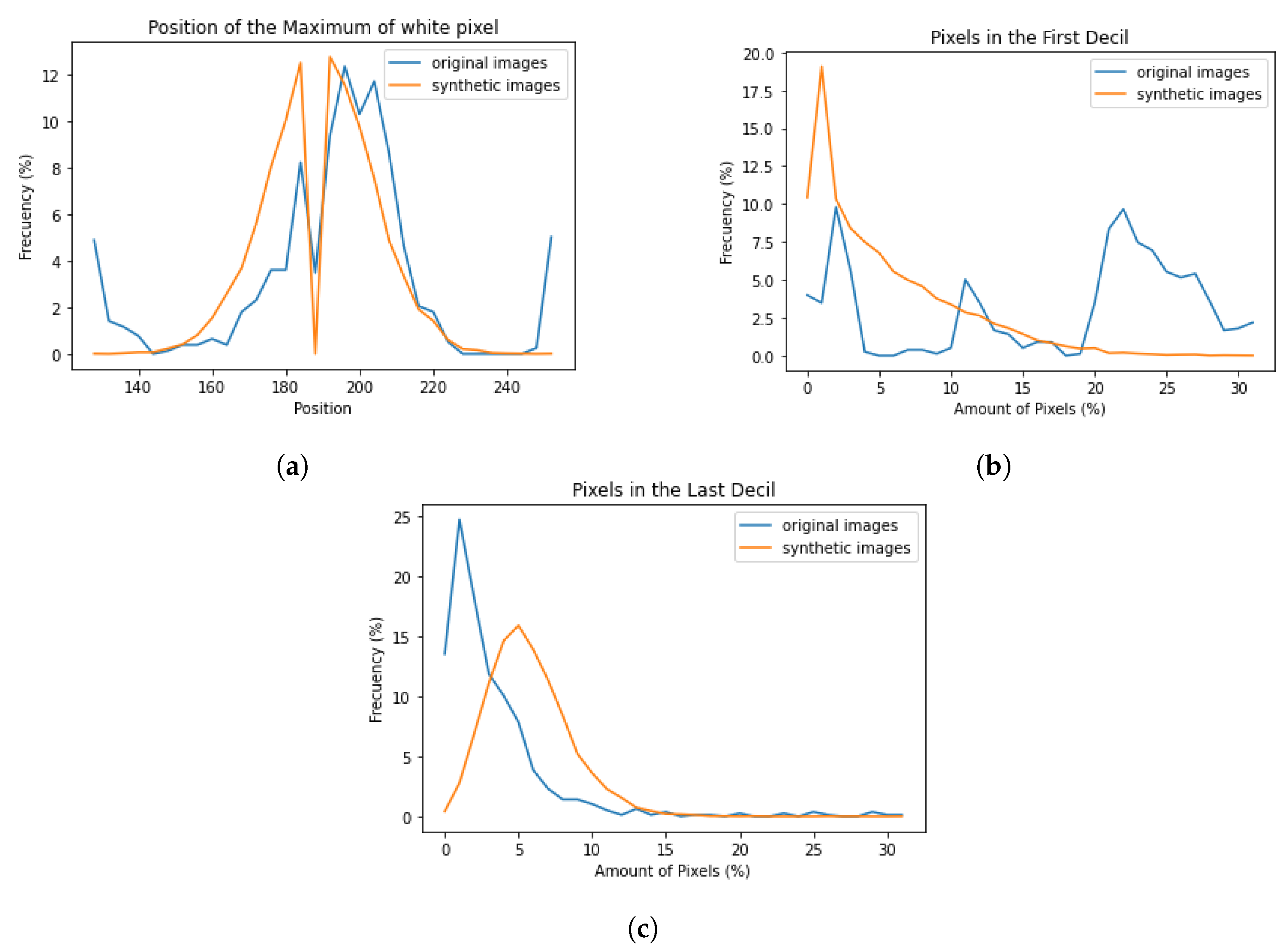
Figure 18a presents a comparison of the histograms of the position of the maximum, found in the right half of the histograms (gray/white colors); it can be seen that both histograms have a similar shape.
Figure 18b presents the histograms of the number of pixels that have low values (up to 10% of the maximum values); it can be seen how the synthetic images do not completely imitate the original ones. A similar case can be seen in
Figure 18c, which represents the histograms of the number of pixels in the last decile; it shows how even if the shapes are pretty similar, there is a shift to the left. It seems this GAN method has some flaws when finding the patterns around the most extreme values. This issue is not critical but shows that this method still has some room to improve.
4.3. Image Quality Metrics
Previous works related to the synthetic generation of EL images of PV cells have not addressed the issue of ensuring the quality of their data by providing objective metrics. The Inception Score (IS) and the Fréchet Inception Distance (FID) are the most important metrics to ensure the quality of synthetic images. In the next paragraphs, both metrics are explained and used. A summary of the results of these metrics can be found in
Table 4.
4.3.1. Inception Score
This metric was first proposed in 2016 [
27] for evaluating the quality of generated artificial images. The score is computed based on the results of a pretrained InceptionV3 model [
28] applied to the generated images. This score is maximized when two conditions are met: The value of the labels is the same for each image, in other words, the entropy of the distribution is minimized. The other condition is that the images are diverse, meaning that the labels are evenly distributed across all possible labels.
For our problem, we used a custom implementation of the metric based on Python and Tensorflow. We compared the results of three different datasets: the original dataset, the synthetic dataset, and a dataset composed only of noise. For each experiment, we split the evaluated dataset into 10 subsets and computed the IS of each one; after that, we computed the mean and the standard deviation. This process reduces the memory cost of the algorithm and the effects of randomness.
The original dataset obtained a mean score of 2.1440 with a standard deviation of 0.0559, the synthetic dataset obtained a mean score of 2.3418 with a standard deviation of 0.4079, and the noise dataset obtained a mean score of 1.0506 with a standard deviation of 0.0026. The results show that both datasets do not obtain a great result with this metric, but their results are better than the results of the noise. This is provoked mostly by the fact that Inceptionv3 was not trained to deal with EL images. It can also be observed that the results of both datasets are similar, with an error of 9.2%. The fact that [
26] produced similar IS values for both shows that they have a high similarity. This proves the quality of the synthetic dataset but also shows that it has some room to improve.
4.3.2. Fréchet Inception Distance
This metric was first proposed in 2017 [
29] to evaluate the quality of synthetic images. In contrast to the IS, this metric compares the distribution of the synthetic data with the distribution of the original data, measuring the similarity between the two datasets.
As in the other case, we used a custom implementation based on Python and Tensorflow. We compared the same three datasets as in the other metric. To compare each dataset with itself, we divided the datasets into two halves after shuffling them. We repeated the process five times in order to reduce the effects of the randomization. The results show that the values of the datasets with themselves were near 0 (0.43118 originals, 0.15095 synthetics, and 2.5117 noise).
We also compared the distance between the three datasets: 15.808 between originals and synthetics, 293.82 between originals and noise, and 296.77 between synthetics and noise. It can be seen that both originals and synthetics are considerably far from noise. It is true that the distance between them is not a value near 0, but it is still a low value, which shows that the difference between both datasets is not high. This is reinforced when this difference is compared with the difference between the noise and both datasets. The difference from 0 is mostly provoked due to the new patterns of shadows and defects that are generated due to the combinations of the different shadows of the original images, thanks to the generative capacity of the DCGAN models.
5. Conclusions and Future Work
The creation of synthetic electroluminescence images of photovoltaic cells is not a trivial problem. Different factors need to be taken into account in order to create high-quality images. The gathering of data is by its nature a manual process, requiring the EL image and its IV curve. The IV curve was measured individually for each cell, which is an innovation from other papers in the bibliography. The obtained images need proper preprocessing in order to perform well in the models. The labeling of the generated data is also a complex problem, since it is not possible to measure the output power or the IV curve of a not-real cell; so, we designed a model to assign a value of performance. This model was trained with the values of the real images, and its low error values show its good performance.
The algorithm used for creating the new images, DCGAN, has shown great performance, not only creating images that are very similar to the originals but also creating new patterns of defects and shadows. This similarity between the original images and the synthetics images was proved using different methods: A visual inspection of the cells shows that they present the characteristics of a real PV cell, and the histogram also proves their similarity, since they share the most important aspects of its shape. Image quality metrics such as Inspection Score (2.3) and French Inception Distance (15.8) also prove their similarity.
The results of this paper prove the quality of the synthetic images, but the dataset can be improved. The most direct way of improving the dataset would be increasing the amount of data. The inclusion of new kinds of defects and shadows would improve the generative capacities of the GAN. Another interesting option would be trying to use different kinds of PV cells, such as monocrystalline PV cells, since our dataset only consists of polycrystalline PV cells. This would improve the usefulness of the dataset in machine learning problems that use other kinds of PV cells.
Another way of improving the quality of the dataset would be increasing the size of the networks. The size of the current networks are based on the limitations in hardware and budget. Bigger networks could reduce the amount of epochs and improve the quality of the generated images. The use of the most innovative architectures could also improve the dataset.

