Abstract
Developing indicators to monitor the dynamic equilibrium of sustainable ecosystem variables has been challenging for policymakers, companies, and researchers. The new method matrix decomposition analysis (MDA) is an adaptation of the Leontief input–output equations for the disaggregated structural decomposition of key performance indicators (KPI). The main problem that this work addresses is related to the behavior of MDA when compared to traditional methodologies such as data envelopment analysis (DEA) and stochastic frontier analysis (SFA). Can MDA be considered robust enough for wide applicability? To compare the models, we developed a methodology called marginal exponentiation experiments. This approach is a type of simulation that raises the inputs and outputs of an entity to a marginal power, thus making it possible to compare a large number of models with the same data. RMarkdown was used for methodological operationalization, wherein data science steps are coded in specific chunks, applying a layered process with modeling. The comparison between the models is operationalized in layers using techniques such as descriptive statistics, correlation, cluster, and linear discriminant analysis (LDA). Given the results, we argue that MDA is a Leontief partial equilibrium model that produces indicators with dual interpretation, enabling the measurement of the dynamic equilibrium of sustainable ecosystem variables. Furthermore, the method offers a new ranking system that detects relative changes in the use of resources correlated with efficiency analysis. The practical value for decision-makers relates to the fact that we found evidence that MDA can be considered robust enough to identify whether a given ecosystem is in equilibrium and that the excessive use of resources or abnormal productivity can cause instability.
1. Introduction
Strategies for achieving sustainability equilibrium are important to both global and local scenarios [1]. One example is the plan for the sustainable economy of the EU, the European Green Deal, which is a growth strategy to protect biodiversity, stimulate the circular economy, create sustainable food, and eliminate pollution [2,3]. According to Frans Timmermans, executive vice president of the European Commission, the COVID-19 crisis revealed the vulnerability of the system and, consequently, the importance of restoring the equilibrium between human activity and nature.
Our work highlights the importance of restoring the equilibrium between economic activity and nature. Developing indicators to monitor the equilibrium is necessary to reduce the level of uncertainty in the formulation of strategies, decisions, or actions [4,5,6,7,8,9,10,11].
The main problem that this research addresses is the scarcity of methodology that indicates whether an ecosystem (enterprise or group of enterprises) is falling out of equilibrium. The quantitative information as to whether a system is out of equilibrium allows the strategist to intervene and make decisions that favor one side or the other. Our approach is somewhat similar to that of classical economics equilibrium (Alfred Marshall) [12], but the latter is static and does not consider all relative changes in the series. The main added value of this research lies in the development and deepening of a methodology that provides objective information if a dynamic system is leaving its temporal equilibrium. The added value of the article is the comparison of this methodology with more traditional ones such as data envelopment analysis (DEA) and stochastic frontier analysis (SFA).
In the literature, reference [10] developed a methodology derived from a Leontief input–output model that may be able to monitor the evolution of sustainability through the analysis of indicators. For simplicity, we identify this methodology by the acronym MDA (matrix decomposition analysis). The MDA method was originally proposed with the possibility of benchmarking analysis in various instances of sustainability science.
The literature addresses two other models that are more often used: data envelopment analysis (DEA) and stochastic frontier analysis (SFA). The origin of DEA is in operational research using mathematical programming, and SFA originates from econometrics, which uses regression techniques. MDA is descended from general economic equilibrium models that use matrix techniques [13,14,15]. The main research question that guides our work is: Does MDA offer a robust ranking system capable of complementing DEA and SFA approaches?
The objective of this work is to systematically explore the MDA methodology proposed in the literature [10]. As complementary objectives, we establish: (i) operationalize the matrix decomposition analysis (MDA) for multiple inputs using MS-Excel®; (ii) develop a systematic comparison procedure with data envelopment analysis (DEA) and stochastic frontier analysis (SFA); (iii) discuss the application of the MDA methodology for the analysis of dual performance in sustainable ecosystems.
The main justification for the work is related to the fact that the Leontief approach is not fully explored in the literature for the purpose of benchmarking. In reference [10], the method was compared with a simple example of stochastic frontier using one input. In this work, we develop a robust experiment (marginal exponentiation) using multiple inputs. The systematic exploration of the method makes it possible to identify its advantages and disadvantages in relation to DEA and SFA. In addition, it produces evidence of its empirical utility for monitoring performance in sustainable ecosystems.
For the experiment, we use data from the Philippine rice production ecosystem [16]. These agribusiness data have become a benchmark example in the literature [16,17,18,19,20]. The International Rice Research Institute (IRRI) supplied data collected from 43 rice producers in the Tarlac region of the Philippines between 1990 and 1997, forming a panel dataset. We used 4 variables: freshly threshed rice (PROD), planted area (AREA), labor used (LABOR), and fertilizer used (NPK). The PROD is the output, and the AREA, LABOR, and NPK are the inputs.
Based on the results of the experiments, we are convinced that the Leontief partial equilibrium model or MDA might offer a new robust ranking system capable of detecting relative changes in the use of resources, which can be applied to input–output relationships of many organizations. Its stability was tested both by correlations with DEA and SFA and by its discriminating power.
2. Ecosystems Concept and Techniques for Benchmarking
2.1. Ecosystem and Indicators
The indicators are part of a system, as “a system defines a set of bounded interrelated elements with emergent properties and represents it within the context of a paradigm” [21] (p. 4). The elements might be the indicators developed within the paradigm of transdisciplinary sustainability science (TSS) [22]. Indicators are implemented in the processes, as “a process is an approach to achieving a managerial objective, through the transformation of inputs into outputs” [21] (p. 4). Examples of methodologies that produce indicators from the input–output relationship are the traditional methods of benchmarking: data envelopment analysis (DEA) and stochastic frontier analysis (SFA). Matrix decomposition analysis (MDA) was recently developed in reference [10].
A broader perspective concerns the ecosystems where the indicators live. Reference [23] provides a robust review of the concept of ecosystems from the point of view of management: “To provide a product/service system, an historically self-organized or managerially designed multilayer social network consists of actors that have different attributes, decision principles, and beliefs” [23] (p. 55). The authors also establish the boundaries of the ecosystem, identifying four hierarchical classes: industrial ecology (natural resource management by industry), business ecosystem (private firms), platform management (extended and virtual enterprise), and multi-actor network (government, private firms, universities, consumers, entrepreneurs, investors) [23] (p. 52).
In an ecosystem, decision-making might cause unintended results because the actors have different priorities, attributes, beliefs, and experiences. In this ecosystem, both positive (collaboration, symbiosis, and improvement) and negative characteristics (predation, parasitism, and destruction of the whole system) exist [23] (p. 52). These characteristics influence the way that the indicators are interpreted. Although the indicators enable us to reduce uncertainty in decision-making for the ecosystem, sometimes there is resistance to adoption [24,25].
2.2. Techniques for Benchmarking
The MDA adapts the Leontief input–output matrix equations for the simultaneous decomposition of multiple key performance indicators (KPI—Input/Output) [10,26,27,28,29,30,31,32,33,34]. The contribution of each series is measured by the Effects (I and II) and aggregated by and . Briefly explained, the effects measure the contribution of variables to the formation of the indicator. The contribution of the numerator is captured by Effect I and the denominator by Effect II (content and activity effects, respectively). The and may be used both internally (comparing different resources within the organization) and externally (comparing the same resources between organizations), enabling benchmarking between different measurement units, e.g., cubic meter, joule, ton, square meter.
DEA and SFA are the main methods for benchmarking, most frequently applied in the areas of finance, transport, agriculture, utilities, and environmental analysis [35,36,37]. DEA is a mathematical programming technique developed by reference [14], and SFA is an econometric technique developed simultaneously by references [14] and [38]. The literature presents advantages for the DEA: it works with a small sample, having no assumption of efficiency distribution; it does not require a functional form for the data; and it enables modeling with multiple outputs. Regarding limitations, the assumption of the absence of errors and sensitivity to outliers can be mentioned [17,39]. The SFA can measure efficiency while considering the presence of statistical noise. Its main limitations are the assumption of the functional form, needing two error terms and using only one output as the dependent variable [16,17].
Since the development of both techniques in the 1970s, there has been a debate in the literature to know which technique is best suitable to measure performance/efficiency. Several surveys use the techniques together (DEA and SFA), and it is possible to compare the results. They can be separated into two groups. First is those whose main objective is to compare the two methodologies [16,40,41,42]. Within this group, the comparison techniques include Monte Carlo simulation (MCS), root mean square error (RMSE), mean absolute error (MAE), Spearman rank correlation, and bias. There are also works in which comparison is not the main objective, but which use both approaches to obtain robustness in the analysis [43,44,45,46,47,48]. In this group, the main comparison technique is the correlation (Pearson and Spearman correlations) [49].
Based on the results of the surveys of the two groups, the answer to which method (DEA or SFA) is more appropriate for estimating performance is not conclusive. Reference [50] finds a moderate consistency between the two approaches, while reference [51] establishes that SFA outperforms DEA for small measurement errors, whereas DEA beats SFA as the measurement errors increase. Reference [16] identifies that combination approaches, such as taking the maximum or the mean over DEA and SFA efficiency scores, might offer a useful alternative to strict reliance on a singular method. The correlation between the two approaches also depends on the model chosen, varying between 0.23 and 1.0; normally, most of the correlations are in the range (0.70–1.0) [44,45,46,47].
3. Materials and Methods
Experiment Design
The methodological process is guided by the general theory of data analysis by reference [48], in which data analysis consists of an investigative process used to extract knowledge, information, and insights from reality; in other words, it is a sensemaking task that updates a given schema using data to fit a model [48]. Our main objective is the exploration of a data set in order to analyze and compare MDA with the DEA and SFA methods [10,14,15]. Inspired by a toy example that used fictitious data, we developed a procedure called the marginal exponentiation experiment, which consists of raising the inputs and outputs to the power of a marginal exponent and observing what happens with the results. Marginal exponentiation is applied in DEA, MDA, and SFA modeling.
Figure 1 describes the methodological process coded in the RMarkdown analytic framework using several steps from data science (import, tidy, transform, view, model, program, and communicate) implemented through chunks [50]. In stage 1, the indicators for MDA, DEA, and SFA are computed by a type of simulation that raises the inputs and outputs of the farms to a marginal power, generating matrices for the analysis process. For MDA, the values and are calculated; for SFA, the functional forms log (SFA-LOG) and translog (SFA-TRANSLOG) are estimated; and for DEA, the models’ constant return to scale input-oriented CRS (DEA-IN) and constant return to scale output-oriented CRS (DEA-OUT) are computed. The experiments were modeled mathematically according to Equations (1)–(3). The indicator matrices generated by the experiments were analyzed using correlation (2), cluster (3), linear discriminant analysis (LDA) (4), and verification of asymptotic convergence (5). The analysis proposition is similar to the layered grammar of graphics, where the parts of a graph are added layer after layer according to the needs of the analysis [48,50,52].
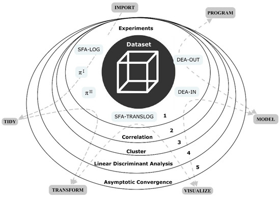
Figure 1.
Methodological layers of data science. Note: Implemented in RMarkdown.
Experiment 1 contains the MDA equations, assuming that lines 3, 4, and 5 are the same equations presented in reference [10]. Marginal exponentiation occurs because the inputs (X) and outputs (I) are raised to the power of so that the higher the value of k, the lower the exponent. The k constant is necessary so that the inputs and outputs are not explosive and so that the value of δ varies in the range [1, N]. The objective of the experiment is to obtain new values for and for each value of δ.
Experiment 1—marginal exponentiation for matrix decomposition analysis (MDA). Note: Proportional coefficients; —input matrix; j—type of input used; —equivalent to Leontief inverse; P—performance indicators; PF—performance flow indicators; t—time; —aggregate dimensionless effect for numerator; —aggregate dimensionless effect for denominator; —diagonal matrix of inverse output; —special output matrix (upper bidiagonal matrix); —difference.
Experiment 2 was operationalized in the same way as Experiment 1, except for use of the Cobb–Douglas log-linear model (SFA-LOG) on line 3 and the translog model on line 4. SFA is a parametric (econometric) technique that estimates the stochastic frontier (assuming random residuals). It was developed simultaneously by Aigner et al. [13] and Meeusen and van Den Broeck [38] and can be represented mathematically in Cobb–Douglas and translog form by Equations (2)–(3) and (2)–(4), respectively, where x represents the output and y the inputs of the system. SFA is estimated using the principle of maximum likelihood [18,19,35,53,54].
Experiment 2—marginal exponentiation for stochastic frontier analysis (SFA). Note: —panel dependent variable; —intercept/coefficients; ——panel independent variables.
Experiment 3 follows the same rationality as Experiment 1 and 2 but is applied to DEA (DEA-IN-DEA-OUT). DEA is a technique that determines the efficiency frontier through mathematical programming; therefore, it is non-parametric. It was developed by Charnes et al. [14] and can be seen in Equation (3) as a minimization problem (input-oriented) where X represents the input(s) under evaluation; Y the output(s) under evaluation; θ the efficiency; and the coefficients. It is also possible to develop the maximization problem (output-oriented). The advantage of DEA lies in its flexibility, and it can even be modeled in spreadsheets [17,18,54,55].
Experiment 3—marginal exponentiation for data envelopment analysis (DEA). Note: — input(s) under analysis; ——output(s) under analysis; —efficiency; —coefficients.
The layers 2 to 5 of Figure 1 are proposed to analyze the results of the experiments, first through the correlation (Pearson and Spearman), then the cluster analysis is applied to confirm the result of the correlation (Equation (4)). For the cluster, we use the sum of the squared Euclidean distances between each data point and the centroid of the subset , which contains . Euclidean distance was chosen due to its popularity, but we emphasize that other possibilities exist in the literature [56,57,58,59].
Discriminant analysis (LDA) was applied to check the possibility of forecasting the indicators generated by the experiments. In practice, LDA will compare the discriminating potential of each indicator [59,60,61]. The prediction errors in a supervised approach are used as a metric to check the randomness of the results of the experiments. Linear discriminant analysis (LDA) is a technique for dimensionality reduction problems as a preprocessing step for machine learning and pattern classification applications. The algorithm for LDA class-dependent is presented by reference [62] in Equations (5)–(8).
First, we calculate the mean of each class and the total mean as Equations (5) and (6), respectively (considering a set of N samples ). After calculating the between-class matrix (Equation (7)), compute the within-class matrix (Equation (8)) [62,63]. Finally, to test the limits of and , an asymptotic test is performed to verify their convergence. This test consists of generating increasingly larger values of N in Equation (1) so that the asymptotic behavior of and can be observed.
4. Results of the Systematic Experiments
4.1. Experiment—Toy Example
The study by reference [10] assigned the Fibonacci sequence to the energy input, identifying that the MDA model works appropriately with extreme values. In this study, six hypothetical situations are considered in Table 1 (A–F). In situation A, the value of the input is equal to the output raised by a power (2,3,4); in this case, the greater potentiation in the input causes an increase in and decrease in , with both remaining in the range [0, 1]. Case D is the same experiment, but for outputs in reverse order; the changes now reflect that the values are clearly out of range [0, 1]. In situation B, the inputs are multiplied by the values (1,2,3). For this case, firstly, if the values of the inputs and outputs are equal, and will be in equilibrium with the value of 0.50; second, the multiplication of the inputs by higher values does not change the indicators; therefore, only relative changes are able to change the indicator. Case C is similar to case B, with outputs in reverse order and values of and also outside the range [0, 1]. For case E, the inputs are considered constant, and for F, the outputs are constant. In these situations, for any value of the constant, in both cases, the values of and do not change, but are [0 and 1] for case E and [1 and 0] for case F.

Table 1.
Toy example for and (MDA).
4.2. Real Example for MDA Model in Excel
The toy example describes hypothetical situations enabling the understanding of the behavior of indicators and . For the next implementations, we use data from the Philippine rice production ecosystem. According to reference [16], these agribusiness data have become a benchmark example in applied efficiency analysis. In the literature, several studies have used these data to test models [16,17,18,19,20]. We used the same methodological implementation as reference [19]: tons of freshly threshed rice (PROD), area planted (AREA), labor used (LABOR), and fertilizer used (NPK). See reference [17] and Supplementary Material for a complete description of the data.
In reference [10], a web application was developed using the R-Shiny script language. In this work, we implemented MDA via RMarkdown and MS-Excel®. Figure 2 shows the calculation flow and Excel® formulas needed to implement MDA equations in 10 steps.
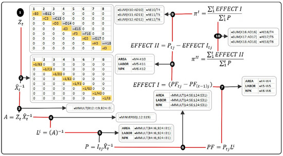
Figure 2.
Calculation flow in Excel for MDA. See note in Equation (1).
Figure 3 presents the results and the information can be found in the Supplementary Material (RMarkdown-Analytics). In quadrant A of the graph, the value of is greater than ; in other words, for six farms, the activity effect (contribution of production) surpassed the content effect (contribution of inputs). In quadrant B, becomes greater than ; in this case, the content effect is greater than the activity effect for 26 farms. In quadrant C, the content effect is enough to make the activity negative.
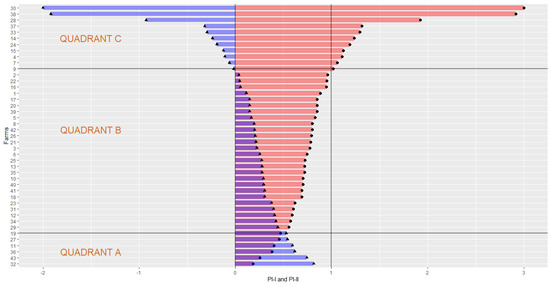
Figure 3.
(dot), (triangle) for rice production in 43 Philippine farms. Note: average of area, labor, and NPK; incomplete visualization farm 38 = 2.92; farm 30 = 11.35; = −1; code in chunk 06.
The MDA does not just generate the aggregate effects ( and ); it is also possible to view the effects for each period, shown in Figure 4 (for more details about the effects see reference [10]).
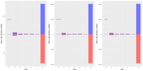
Figure 4.
Effect I and Effect II for farm 30. Note: AREA ; NPK ; LABOR ; code in chunk 07.
According to the graph in Figure 4, Effect I can be considered an outlier in period 8 for all inputs (AREA, LABOR, and NPK). The outliers may be justified because the production of farm 30 fell from 1.06 tons in the year 7 to 0.09 in year 8; in other words, a reduction of more than 1000%. To fix the analysis, the reduction in inputs was less than proportional for this period (AREA = 60%, NPK = 174%, and LABOR = 238%). It is interesting to note that the values of and carry the entire change history; therefore, extreme values should be investigated. This same procedure could be applied to other farms.
4.3. Marginal Exponentiation Experiment
The marginal experiments were presented in level 1 of Figure 1 and are mathematically described in Equations (1)–(3). The analytical process was implemented via RMarkdown using 19 chunks [see Supplementary Materials in RMarkdown-Analytics (.rmd; .pdf)]. The experiments for the DEA and MDA were also modelled in Excel-VBA, generating the same results as in RMarkdown (chunk 01). For comparison feasibility, farm averages for DEA and SFA in the period were calculated. After several tests that considered the computational capacity of the packages, the parameter values N = 40 and k = 10 were chosen for the three experiments. This means that both inputs (AREA, LABOR, NPK) and output (PROD) are raised to the fourth power with a step of 0.10. It was possible to calculate 40 observations for each farm, totaling 40 × 43 = 1720 data points for each indicator (SFA-LOG, SFA-TRANSLOG, DEA-IN, DEA-OUT, and ). The experiments enabled the computation of 80 models for SFA, 1720 models for MDA, and 3440 DEA models. For SFA, there are only 80 because the panel structure was used (40 × 2) (log, translog); in the case of MDA, the computation was realized for each farm separately (40 × 43); in the same way as MDA, the DEA calculation was made individually for input/output-oriented models (40 × 43 × 2). The results of the experiments are found in the Supplementary Materials, totaling 5240 models that generate 1720 × 6 = 10,320 performance measurement points (see RMarkdown-Analytics).
Figure 5 shows the stacked histogram for the real performance of the 43 farms. In the experiments, the real indicators are obtained when the value of δ is equal to 10 in Equation (1) (); since k = 10, we have , obtaining the dataset without potentiation. It can be noted that most models have performance values in the range [−1, 2]. An exception is farm 30, which is in the range [11, 12] for and [−11, −10] for .
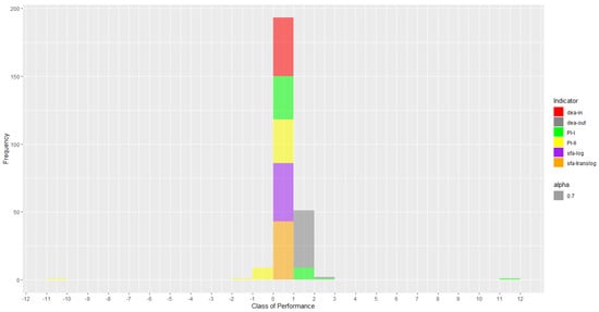
Figure 5.
Histogram of SFA-TRANSLOG, SFA-LOG, DEA-OUT, DEA-IN, , and . Note: code in chunk 08.
Figure 6 shows the distribution of each indicator through boxplots, aggregating 43 farms by average. The mean is affected by outliers, appearing in , , and DEA-OUT. Figure 7 and Figure 8 show that the distortions are being caused by farms 28, 30, and 38.
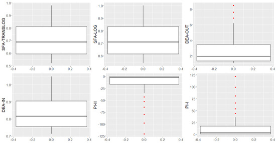
Figure 6.
Boxplots of SFA-TRANSLOG, SFA-LOG, DEA-OUT, DEA-IN, , and . Note: code in chunk 09.
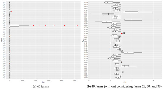
Figure 7.
Boxplots for . Note: code in chunk 10.
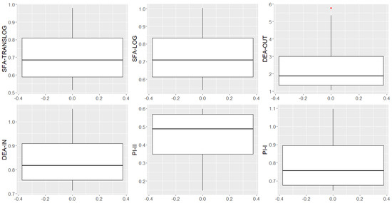
Figure 8.
Boxplots for SFA-TRANSLOG, SFA-LOG, DEA-OUT, DEA-IN, , and . Note: 40 farms (without considering farms 28, 30, and 38); code in chunk 11.
In order to check the correlation between the six indicators matrices (40 × 43) of the results of the experiments (Equations (1)–(3)), both Spearman’s rank correlation and Pearson’s product–moment correlation with pairs of the matrices were calculated. (Using Spearman’s method, most individual correlations have values equal to 1). The complete results are in the Supplementary Material (chunks 18 and 19). Interestingly, there are positive and negative correlations. For the indicator pairs [, , () and ], the correlation is negative for ten farms and positive for the others, being the opposite for the pairs [, , , ].
Figure 9 adds the correlation (), captured from the diagonal of the correlation matrix (same farm between indicators) (for more details, see chunks 18 and 19). One issue to explain is the positive and negative differences in correlations. The graph in Figure 9 shows that when the value of is greater than 1, the correlation is negative, whereas the opposite occurs when the value is less than 1; an exception is farm 15. Based on reference [10], and measure the aggregate effects associated with the total changes in inputs and outputs, respectively (the toy example clarifies this assertion). Since measures the content effect and the activity effect, for the farms in quadrant C of Figure 9, the content effect was more than proportionally greater than the activity effect. This evidence suggests that marginal exponentiation amplified the effects on ; in other words, it amplified the stochastic structure already existing in the data of this ecosystem.
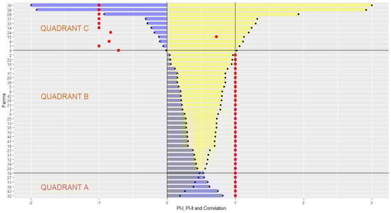
Figure 9.
(dot), (triangle), and Spearman’s rank correlation (, DEAIN) (square). Note: p-value = 2.2 × 10⁻¹⁶, the same pattern occurs with Pearson’s correlations, but with most correlations less than 1; code in chunk 12.
Basically, what we want to highlight is that the graph in Figure 9 shows that the correlation is negative for farms that have a greater aggregate content effect ( in quadrant C); in other words, those farms used proportionally more resources (AREA, LABOR, and NPK) to produce the same amount of rice. This interpretation is compatible with the efficient use of resources. Interestingly, the threshold occurs exactly where the value of becomes negative. An exception is farm 15, but with a lower positive correlation than other farms.
To distinguish the 43 farms in relation to the indicators and , we apply the K-means clustering technique [64]. In the clusters of Figure 10, a clear distinction of eight farms can be identified (7, 14, 24, 28, 30, 33, 37, 38), all belonging to quadrant C of Figure 3 and Figure 9.
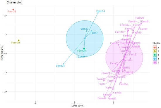
Figure 10.
Farm clusters for the indicator. Note: code in chunk 13.
To complete the analysis of the correlations, Figure 11 and Figure 12 present the visualization matrix with the correlations (upper), density function (diag), and scatterplot of the indicators (lower). It can be noted that all correlations are statistically significant, but with an inversion of signs when the value of becomes negative; in other words, farms that are in quadrant C, except for farm 15. This means that the result in Figure 9 for () can be generalized for all indicators.
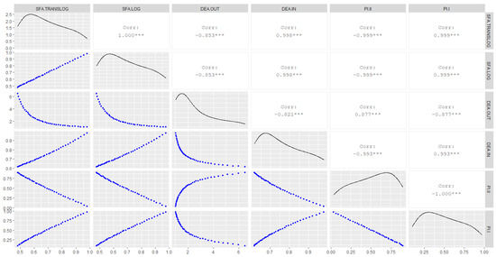
Figure 11.
Correlation matrix of indicators. Note: *** p-value is < 0.001; considering the average of the farms in quadrant A and B of Figure 9 (plus farm 15); code in chunk 14.
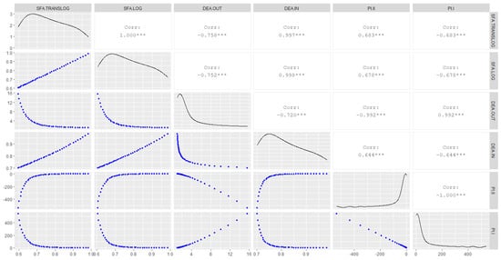
Figure 12.
Correlation matrix of indicators. Note: “***” p-value is < 0.001; considering the average of the farms in quadrant C of Figure 9 (minus farm 15); code in chunk 15.
An additional question is whether and of the MDA method has the same discriminating potential as the indicators generated in the DEA and SFA approaches and can be predicted with similar accuracy. This may indicate that the results of MDA are not random. Our work uses linear discriminant analysis (LDA) because it is a technique often used in the literature that operates with nonmetric dependent variables [62]. Table 2 shows the LDA confusion matrix implemented in the R caret package and coded in chunk 16 [65].
Table 2.
LDA confusion matrix.
The operationalization of the LDA would have multicollinearity problems if we used all 43 farms as dependent variables; therefore, we adopted the following procedure: an RMarkdown script was developed that randomly selects 5 farms where the indicator is the categorical dependent variable (6 categories) and the farms are the independent variables. Table 2 shows the average of 30 LDA models to reduce the presentation of the results. The overall accuracy of the models was 91%. In Table 2, the values generated by the MDA model ( and ) are at least as stable as those generated by DEA or SFA (the complete result is in chunk 16 of RMarkdown).
A final analysis identified in Figure 1 refers to the asymptoticity of and . It is not possible to observe in the previous examples because the comparison occurred in the range [1,40]. For checking asymptoticity, among the packages used, the best performance was the matrix inversion of Excel, combined with VBA, allowing us to test the behavior of and with N = 500 for the 43 farms. With the reduction factor , the maximum power was 50, being enough to verify the convergence. The graphs in Figure 13 show the behavior of the indicators for farms 1, 4, 10, and 24.
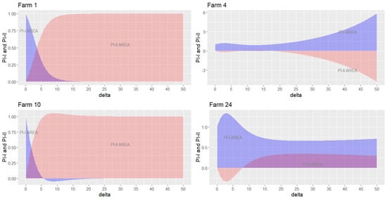
Figure 13.
Asymptotic convergence for farms (1, 4, 10, and 24). Note: code in chunk 17.
The visualization of farms 1 and 10 shows that when the parameter δ increases, tends to 0 and tends to 1. This result can be generalized to 29 farms, understood as a long-term stochastic behavior. For these farms, the structure of the data indicates that, in the long run, the activity effect has a dominance over the content effect. The farm 4 graph indicates a dominance of the content effect that can be generalized to 9 farms. The behavior of farm 24 represents a group of 5 farms in which the effects are divided into the interval [0, 1].
5. Discussion
In this research, we systematically explored the MDA method, where the main objective was to verify its robustness when compared to DEA and SFA. First, a toy example was built to demonstrate the behavior of and given a certain class of hypothetical variation in input and output. Second, the model was operationalized in MS-Excel® using data from an agribusiness ecosystem. Subsequently, three experiments were developed to compare MDA with DEA and SFA (marginal exponentiation). The implementation occurred through the development of chunks in the RMarkdown framework. As described in reference [10], the indicator measures the contribution of input (content effect) and the contribution of output (activity effect) over time. To understand these effects, we can imagine that is on one side of a seesaw and on the other side, but with the difference that the seesaw will only oscillate with proportionally different weights. According to the toy example, only the relative changes in input and output can change the indicators (situations A and D in Table 1).
Multiplying the output by any scalar does not change the relative distance of the series and therefore does not change the indicator (situations B and C in Table 1). In situations C and D, there is a disequilibrium due to the decrease in output. Cases E and F are specific situations of equilibrium of our hypothetical seesaw, where for case E, all weight of change accumulates on the output [ and ], and the reverse for the input in the situation F [1 and ]. By looking at the toy example, we can argue that the maximum equilibrium difference will always be 1 [10].
It was proposed in reference [10] that and might be used for internal and external benchmarking in sustainability science. It is possible to compare which decision-making unit (DMU) had the greatest aggregate content effect (). For example, if we want to analyze the use of energy, water, or emissions, a higher reflects a greater aggregation of content in the production of goods or services.
Figure 3 shows the benchmarking for 43 rice-producing farms using the resources (AREA, LABOR, and NPK). Quadrant A revealed farms with greater activity by means of . The farms in quadrant B are those with the lowest activity, and those in quadrant C are those with negative activity (related to the evolution of rice production). Another perspective is the utilization of resources (. Figure 3 also ranks farms in ascending order of resource utilization. The graphs in 3 reveal that extreme cases can be inspected by analyzing Effects I and II. An extreme change can also mean an error in the data (for more information about the effects see reference [10]).
In reference [10], the MDA approach was compared with SFA, identifying a negative correlation of −0.80 and −0.40 between and the SFA. However, these are just two isolated examples needing a more robust experiment for detailed comparison. The inspiration for the development of the marginal exponentiation experiment was derived from the observations of the toy example, initiated in reference [10]. Considering that exponentiation changes the relative distance of the series (inputs, outputs), it is possible to use multiple databases to compare the behavior of indicators of different models in a controlled manner. The MDA model was compared to DEA and SFA efficiency analyses.
From the distributions shown in the boxplots of Figure 6, it can be noted that there was less variability for the DEA-IN, SFA-LOG, and SFA-TRANSLOG models when compared to the models (, , DEA-OUT). In Figure 7 and Figure 8, it can be noted that the asymmetries are caused by farms 28, 30, and 38.
The main finding of the correlations is shown in Figure 9, considering (DEA-IN, ) to exemplify thatmost farms have a positive correlation with the efficiency indicator (quadrant A and B), but some have a negative correlation (quadrant C). This result momentarily differentiates the MDA approach from DEA and SFA since 10 farms have a positive correlation and 33 have a negative correlation with efficiency. Since the application of the three experiments followed identical rules, there is evidence to suspect a stochastic pattern in which the data were generated in this ecosystem, captured by the MDA method. The stochastic pattern in the data was potentialized by the experiment (marginal exponentiation). The most plausible explanation for this difference is the fact that farms with the highest content effect () are negatively correlated with efficiency and that farms with the least content effect are positively correlated. The threshold is shown in Figure 9; when the value of becomes negative, the content effect dominates the activity effect.
Cluster analysis identifies that the majority of farms belonging to quadrant C in Figure 9 form distinct clusters from farms that are in quadrants A and B. Correlations are also inverse for and and between DEA-IN and DEA-OUT, as expected. The application of LDA confirms similar forecasting chances, statistically significant among the three models (DEA, MDA, and SFA). The asymptotic test shows that there is a long-term pattern for the behavior of and . It was not possible to verify the asymptotic behavior for DEA and SFA due to model errors caused by computational complexity. It seems probable from these results that MDA can work consistently with more extreme conditions than can DEA and SFA.
We must emphasize that MDA does not have assumptions of optimization (maximum-likelihood estimation or mathematical programming). The estimation of and is based on an indicator decomposition approach derived from Leontief’s input–output model [12,22,48]. Part of the decomposition is attributed to the inputs () and part to the outputs (); therefore, we think it is reasonable to assume that MDA is a Leontief partial equilibrium model that produces dual indicators. The duality of the indicators and is related to the content and activity effects discussed in reference [10]. Interpreted from another point of view, the content effect is related to efficiency (INPUT/OUTPUT) and the activity effect on productivity (OUTPUT/INPUT). In the case of efficiency, we want to reduce the use of resources (AREA, LABOR, and NPK) per unit of output (rice) and, in the second case, we seek to increase the output (rice) per unit of input. The indicators and seek to measure this duality.
In both the toy example and rice production analysis, there are situations of disequilibrium concerning the productivity and efficiency; in other words, content and activity effects. From the point of view of sustainable management, this disequilibrium is related to resource management versus output management. In practical terms, duality unveils the condition of production with minimal impact on the environment that at the same time meets the need for financial results with the achievement of productivity. The MDA method reveals the minimization/maximization effort over a certain period.
The MDA methodology has the potential to quantify the duality existing in an ecosystem for a given period. Figure 14 highlights the MDA contribution to the analysis of performance in sustainable ecosystems.
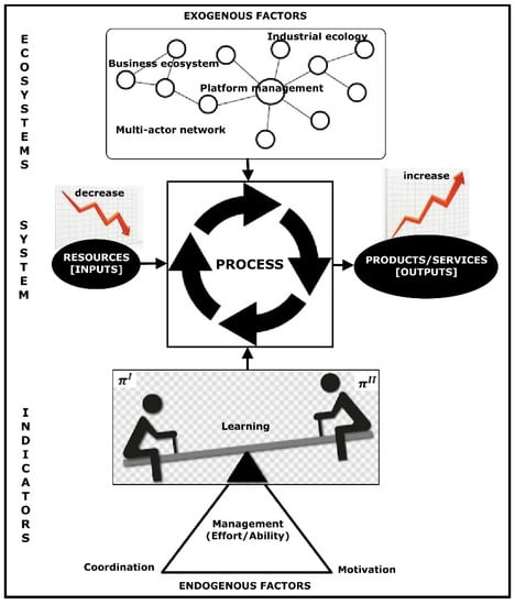
Figure 14.
Dual performance in sustainable ecosystems.
MDA enabled benchmarking across indicators with different units of measurement, e.g., cubic meter, joule, ton, square meter [10]. The main application discipline of MDA is transdisciplinary sustainability science (TSS) [16]. In this work, we introduce the notion of ecosystems in which the indicators live (industrial ecology, private firms, platform management, and multi-actor network). The indicators are created in systems with dual processes (increase, decrease) belonging to a given ecosystem, providing learning (benchmark), coordination (allocation of tasks), and motivation (reduction of uncertainties) [10,15].
As in the DEA and SFA approaches, MDA has the possibility of expanding to other contexts that use the input–output relationship in economic, social, and environmental processes, with the limitation of working with time series. The advantage lies in the flexibility of the measurement and the decision-making duality in each ecosystem. The results seem to demonstrate that although the MDA has a high correlation with efficiency (DEA, SFA), the comparison must consider that the MDA is a dual benchmarking system.
The work is about a new method that still needs to be tested many times before we can understand the final conclusion about all application possibilities. The idea of this comparison is to test whether MDA can be as robust as DEA or SFA. Once its robustness is tested, the practical relevance can be wide because in fact we believe that we have discovered a mathematical matrix property for the study of variables in ecosystem equilibrium. In the case of this work, the equilibrium of production factors in a specific production process (rice production) was tested. Generally, MDA can be applied to analyze the equilibrium of production factors in other sectors, such as industrial and commercial. A contribution can be made to the study of the equilibrium of natural resources that involves sustainability.
6. Conclusions
We conclude that MDA might be as stable as DEA and SFA approaches, but captures the dual performance, measuring the Leontief partial equilibrium of the variables of interest, enabling practitioners and decision-makers to make necessary adjustments. MDA has the capacity to identify whether a given ecosystem is in equilibrium. The instability can be caused by the excessive use of resources or abnormal productivity. When two entities are compared, it is evident whether one or the other phenomenon is occurring. This is what we called dual benchmarking.
Some aspects can be highlighted in relation to the results: (i) only relative changes in input and output can change the indicators; therefore, multiplying the input/output by any scalar does not change the indicator; (ii) the distribution of the results of MDA shows greater asymmetries when compared to DEA/SFA, which on the one hand provides greater discrimination, but on the other, there is a need to examine the cases of outliers through Effect I and Effect II; (iii) there is a correlation between MDA and the efficiency models (DEA, SFA), but the sign depends on a certain threshold in the use of resources. For this study, the threshold occurs when the aggregate activity effect becomes negative; (iv) MDA does not start from optimization assumptions like DEA and SFA do, being a Leontief partial equilibrium model that produces dual indicators, offering a ranking system capable of detecting relative changes in the use of resources. MDA enables conflict resolution in terms of gains and losses over time.
The original contribution of the article is related to the proposal of a computational approach that demonstrates the duality of KPI indicators. The intention was to show that the MDA is robust, and we generated evidence that this model can be generalized to multiple ecosystems, once we stressed its capacity using exponential functions.
The main limitation of this article is related to the MDA model concerning DEA–SFA. MDA works only with time series data and is not operationalized for cross-sections. Another limitation is that MDA works with the decomposition principle and DEA and SFA with the optimization principle, which brings challenges to the comparison. Although the directions are different, the models are based on the theory of production (MDA is based on Leontief’s general equilibrium production model andDEA–SFA are based on the production function of the theory of the firm).
We believe that future studies can be developed using other techniques of comparison such as simulation. Given the stability of MDA evident in this work, a promising area for future research would probably be in applied studies to measure the dynamic equilibrium of the sustainable ecosystem variables. In practice, the objective of this work was to verify whether MDA has as much stability as DEA and SFA; instead of using the simulation, we used marginal exponentiation, which is not common in the literature. For future studies, a comparison of marginal exponentiation with a Monte Carlo simulation model is challenging. On the other hand, the development of MDA to work with cross-sectional data could bring good results. We also suggest the development of axioms of mathematical theory that support the empirical study carried out.
Supplementary Materials
The following supporting information can be downloaded at: https://www.mdpi.com/article/10.3390/su15086744/s1.
Author Contributions
Conceptualization, M.G.P. and F.M.R.; methodology, M.G.P. and C.P.d.V.; software, M.G.P. and W.V.d.S.; validation, M.G.P., Z.S. and C.P.d.V.; resources, C.P.d.V.; data curation, M.G.P. and W.V.d.S.; writing, original draft preparation, M.G.P., Z.S. and W.V.d.S.; writing, review and editing, M.G.P., F.M.R., Z.S., C.P.d.V. and W.V.d.S.; visualization, Z.S. and W.V.d.S.; supervision, C.P.d.V.; project administration, M.G.P. and C.P.d.V. All authors have read and agreed to the published version of the manuscript.
Funding
The authors Veiga and Silva thank the National Council for Scientific and Technological Development—CNPq, Brazil (Grants number: 312023/2022-7-PQ, and 302407/2022-7 PQ) for its financial support of this work.
Institutional Review Board Statement
Not applicable.
Informed Consent Statement
Not applicable.
Data Availability Statement
The datasets used and/or analyzed during the current study are available in the supplementary material.
Acknowledgments
The authors wish to express their gratitude to the editors and reviewers for their constructive input and insightful feedback.
Conflicts of Interest
The authors declare no conflict of interest.
References
- Fang, K. Moving away from sustainability. Nat. Sustain. 2022, 5, 5–6. [Google Scholar] [CrossRef]
- EC-European Commission. EU Biodiversity Strategy for 2030: Bringing Nature back into our Lives, Brussels, 20.5.2020. Available online: https://eur-lex.europa.eu/legal-content/EN/TXT/?uri=CELEX:52020DC0380 (accessed on 20 November 2022).
- EC-European Commission. The European Green Deal–Brussels, 11 December 2019. Available online: https://commission.europa.eu/strategy-and-policy/priorities-2019-2024/european-green-deal_en (accessed on 20 November 2022).
- Warhurst, A. Sustainability Indicators and Sustainability Performance Management, WBCSD, Report; University of Warwick: Coventry, UK, 2002. [Google Scholar]
- Joung, C.B.; Carrell, J.; Sarkar, P.; Feng, S.C. Categorization of indicators for sustainable manufacturing. Ecol. Indic. 2012, 24, 148–157. [Google Scholar] [CrossRef]
- Hassini, E.; Surti, C.; Searcy, C. A literature review and a case study of sustainable supply chains with a focus on metrics. Int. J. Prod. Econ. 2012, 140, 69–82. [Google Scholar] [CrossRef]
- Hák, T.; Janoušková, S.; Moldan, B. Sustainable development goals: A need for relevant indicators. Ecol. Indic. 2016, 60, 565–573. [Google Scholar] [CrossRef]
- Machado, C.G.; Pinheiro de Lima, E.; Gouvea da Costa, S.E.; Angelis, J.J.; Mattioda, R.A. Framing maturity based on sustainable operations management principles. Int. J. Prod. Econ. 2017, 190, 3–21. [Google Scholar] [CrossRef]
- Schmidt-Traub, G.; Kroll, C.; Teksoz, K.; Durand-Delacre, D.; Sachs, J.D. National baselines for the Sustainable Development Goals assessed in the SDG Index and Dashboards. Nat. Geosci. 2017, 10, 547–555. [Google Scholar] [CrossRef]
- Perroni, M.G.; Tortato, U.; Vieira da Silva, W.; Pereira da Veiga, C.; Senff, C.O. Analytical method for sustainability science benchmarking: An indicator decomposition approach. Ecol. Indic. 2020, 116, 106470. [Google Scholar] [CrossRef]
- Qiu, J.; Zipper, S.C.; Motew, M.; Booth, E.G.; Kucharik, C.J.; Loheide, S.P. Nonlinear groundwater influence on biophysical indicators of ecosystem services. Nat. Sustain. 2019, 2, 475–483. [Google Scholar] [CrossRef]
- Marshall, A. Principles of Economics (1890)–Founder of Modern (Neo-Classical) Economics; Digireads.com Publishing: Overland Park, KS, USA, 2012; 534p. [Google Scholar]
- Leontief, W.W. Input-Output Economics; Oxford University Press: Oxford, UK, 1966; p. 257. [Google Scholar]
- Aigner, D.; Lovell, C.K.; Schmidt, P. Formulation and estimation of stochastic frontier production function models. J. Econom. 1977, 6, 21–37. [Google Scholar] [CrossRef]
- Charnes, A.; Cooper, W.W.; Rhodes, E. Measuring the efficiency of decision making units. Eur. J. Oper. Res. 1978, 2, 429–444. [Google Scholar] [CrossRef]
- Andor, M.A.; Parmeter, C.; Sommer, S. Combining uncertainty with uncertainty to get certainty? Efficiency analysis for regulation purposes. Eur. J. Oper. Res. 2019, 274, 240–252. [Google Scholar] [CrossRef]
- Coelli, T.J.; Rao, D.S.P.; O’Donnell, C.J.; Battese, G.E. An Introduction to Efficiency and Productivity Analysis; Springer: Berlin/Heidelberg, Germany, 2005. [Google Scholar]
- O’Donnell, C.J. Productivity and Efficiency Analysis: An Economic Approach to Measuring and Explaining Managerial Performance; Springer: Brisbane, QLD, Australia, 2018; 418p. [Google Scholar]
- Henningsen, A. Introduction to Econometric Production Analysis with R (Fourth Draft Version); Department of Food and Resource Economics, University of Copenhagen: Copenhagen, Denmark, 2019. [Google Scholar]
- Rho, S.; Schmidt, P. Are all firms inefficient? J. Product. Anal. 2015, 43, 327–349. [Google Scholar] [CrossRef]
- Shehabuddeen, N.; Probert, D.; Phaal, R.; Platts, K. Representing and Approaching Complex Management Issues: Part 1—Role and Definition; Working Paper Series; University of Cambridge Institute for Manufacturing: Cambridge, UK, 1999. [Google Scholar]
- Brandt, P.; Ernst, A.; Gralla, F.; Luederitz, C.; Lang, D.J.; Newig, J.; Reinert, F.; Abson, D.J.; Von Wehrden, H. A review of transdisciplinary research in sustainability science. Ecol. Econ. 2013, 92, 1–15. [Google Scholar] [CrossRef]
- Tsujimoto, M.; Kajikawa, Y.; Tomita, J.; Matsumoto, Y. A review of the ecosystem concept—Towards coherent ecosystem design. Technol. Forecast. Soc. Change 2018, 136, 49–58. [Google Scholar] [CrossRef]
- McAfee, A.; Brynjolfsson, E. Big Data: The Management revolution. Harv. Bus. Rev. 2012, 90, 58–68. [Google Scholar]
- Assis, F.G.L.F.; Ferreira, K.R.; Vinhas, L.; Maurano, L.; Almeida, C.; Carvalho, A.; Rodrigues, J.; Maciel, A.; Camargo, C. TerraBrasilis: A Spatial Data Analytics Infrastructure for Large-Scale Thematic Mapping. Int. J. Geo-Inf. 2019, 8, 513. [Google Scholar] [CrossRef]
- Leontief, W.W. Quantitative input and output relations in the economic system of the United States. Rev. Econ. Stat. 1936, 18, 105–125. [Google Scholar] [CrossRef]
- Lin, X.; Polenske, K.R. Input-output modeling production processes for business management. Struct. Change Econ. Dyn. 1998, 9, 205–226. [Google Scholar] [CrossRef]
- Albino, V.; Kühtz, S. Enterprise input–output model for local sustainable development—The case of a tiles manufacturer in Italy. Resour. Conserv. Recycl. 2004, 41, 165–176. [Google Scholar] [CrossRef]
- Albino, V.; Kühtz, S.; Petruzzelli, A.M. Analysing logistics flows in industrial clusters using an enterprise input-output model. Interdiscip. Inf. Sci. 2003, 14, 25–41. [Google Scholar] [CrossRef]
- Albino, V.; Dietzenbacher, E.; Kühtz, S. Analysing materials and energy flows in an industrial district using an enterprise input-output model. Econ. Syst. Res. 2003, 15, 457–480. [Google Scholar] [CrossRef]
- Albino, V.; Izzo, C.; Kühtz, S. Input–output models for the analysis of a local/global supply chain. Int. J. Prod. Econ. 2002, 78, 119–131. [Google Scholar] [CrossRef]
- Miller, R.E.; Blair, P.D. Input-Output Analysis: Foundations and Extensions, 2nd ed.; Cambridge University Press: Cambridge, UK, 2009; pp. 1–750. [Google Scholar]
- Kuhtz, S.; Zhou, C.; Albino, V.; Yazan, D.M. Energy use in two Italian and Chinese tile manufacturers: A comparison using an enterprise input-output model. Energy 2010, 35, 364–374. [Google Scholar] [CrossRef]
- Perroni, M.G.; Gouvea da Costa, S.E.; Pinheiro de Lima, E.; Vieira da Silva, W.; Tortato, U. Measuring energy performance: A process based approach. Appl. Energy 2018, 222, 540–553. [Google Scholar] [CrossRef]
- Coelli, T. Estimators and Hypothesis Tests for a Stochastic Frontier Function: A Monte Carlo Analysis. J. Product. Anal. 1995, 6, 247–268. [Google Scholar] [CrossRef]
- Fried, H.O.; Lovell, C.A.K.; Schmidt, S.S.; Yaisawarng, S. Accounting for Environmental Effects and Statistical Noise in Data Envelopment Analysis. J. Product. Anal. 2002, 17, 157–174. [Google Scholar] [CrossRef]
- Daraio, C.; Kerstens, K.; Nepomuceno, T.; Sickles, R.C. Empirical surveys of frontier applications: A meta-review. Int. Trans. Oper. Res. 2019, 27, 709–738. [Google Scholar] [CrossRef]
- Meeusen, W.; van Den Broeck, J. Efficiency estimation from Cobb–Douglas production functions with composed error. Int. Econ. Rev. 1977, 18, 435–444. [Google Scholar] [CrossRef]
- Fethi, D.M.; Pasiouras, F. Assessing bank efficiency and performance with operational research and artificial intelligence techniques: A survey. Eur. J. Oper. Res. 2010, 204, 189–198. [Google Scholar] [CrossRef]
- Cullinane, K.; Wang, T.-F.; Song, D.-W.; Ji, P. The technical efficiency of container ports: Comparing data envelopment analysis and stochastic frontier analysis. Transp. Res. Part A 2006, 40, 354–374. [Google Scholar] [CrossRef]
- Krüger, J.J. A Monte Carlo study of old and new frontier methods for efficiency measurement. Eur. J. Oper. Res. 2012, 222, 137–148. [Google Scholar] [CrossRef]
- Kuosmanen, T.; Saastamoinen, A.; Sipiläinen, T. What is the best practice for benchmark regulation of electricity distribution? Comparison of DEA, SFA and StoNED methods. Energy Policy 2013, 61, 740–750. [Google Scholar]
- Reinhard, S.; Lovell, C.A.K.; Thijssen, G.J. Environmental efficiency with multiple environmentally detrimental variables; estimated with SFA and DEA. Eur. J. Oper. Res. 2000, 121, 287–303. [Google Scholar] [CrossRef]
- Odeck, J. Measuring technical efficiency and productivity growth: A comparison of SFA and DEA on Norwegian grain production data. Appl. Econ. 2007, 39, 2617–2630. [Google Scholar] [CrossRef]
- Iglesias, G.; Castellanos, P.; Seijas, A. Measurement of productive efficiency with frontier methods: A case study for wind farms. Energy Econ. 2012, 32, 1199–1208. [Google Scholar] [CrossRef]
- Zhou, P.; Ang, B.W.; Zhou, D.Q. Measuring economy-wide energy efficiency performance: A parametric frontier approach. Appl. Energy 2012, 90, 196–200. [Google Scholar] [CrossRef]
- Honma, S.; Hu, J.-L. A panel data parametric frontier technique for measuring total-factor energy efficiency: An application to Japanese regions. Energy 2014, 78, 732–739. [Google Scholar] [CrossRef]
- Grolemund, G.; Wickham, H. A Cognitive Interpretation of Data Analysis. Int. Stat. Rev. 2014, 2, 184–204. [Google Scholar] [CrossRef]
- Field, A.; Miles, J.; Field, Z. Discovering Statistics Using R; Sage Publications: Newbury Park, CA, USA, 2012; p. 1470. [Google Scholar]
- Dong, Y.; Hamilton, R.; Tippett, M. Cost efficiency of the Chinese banking sector: A comparison of stochastic frontier analysis and data envelopment analysis. Econ. Model. 2014, 36, 298–308. [Google Scholar] [CrossRef]
- Oh, S.-C.; Shin, J. The impact of mismeasurement in performance benchmarking: A Monte Carlo comparison of SFA and DEA with different multi-period budgeting strategies. Eur. J. Oper. Res. 2015, 240, 518–527. [Google Scholar] [CrossRef]
- Wickham, H. ggplot2. WIREs Comput. Stat. 2011, 3, 180–185. [Google Scholar] [CrossRef]
- Yang, Z.; Roth, J.; Jain, R.K. DUE-B: Data-driven urban energy benchmarking of buildings using recursive partitioning and stochastic frontier analysis. Energy Build. 2018, 163, 58–69. [Google Scholar] [CrossRef]
- Grolemund, G.; Wickham, H. Visualizing Complex Data with Embedded Plots. J. Comput. Graph. Stat. 2015, 24, 26–43. [Google Scholar] [CrossRef]
- Zhu, J. Quantitative Models for Performance Evaluation and Benchmarking, Data Envelopment Analysis with Spreadsheets, 3rd ed.; Springer: New York, NY, USA, 2014. [Google Scholar]
- Jaccard, P. The distribution of the flora in the alpine zone1. New Phytol. 1912, 11, 37–50. [Google Scholar] [CrossRef]
- Stojanov, D. Phylogenicity of B. 1.1. 7 surface glycoprotein, novel distance function and first report of V90T missense mutation in SARS-CoV-2 surface glycoprotein. Meta Gene 2021, 30, 100967. [Google Scholar] [CrossRef] [PubMed]
- Sorensen, T.A. A method of establishing groups of equal amplitude in plant sociology based on similarity of species content and its application to analyses of the vegetation on Danish commons. Biol. Skr. 1948, 5, 1–34. [Google Scholar]
- Stojanov, D.; Lazarova Veljkova, E.; Rubartelli, P.; Giacomini, M. Predicting the outcome of heart failure against chronic-ischemic heart disease in elderly population–Machine learning approach based on logistic regression, case to Villa Scassi hospital Genoa, Italy. J. King Saud Univ.–Sci. 2023, 35, 102573. [Google Scholar] [CrossRef]
- Ward, A.; Sarraju, A.; Chung, S.; Li, J.; Harrington, R.; Heidenreich, P.; Palaniappan, L.; Scheinker, D.; Rodriguez, F. Machine learning and atherosclerotic cardiovascular disease risk prediction in a multi-ethnic population. NPJ Digit. Med. 2020, 3, 125. [Google Scholar] [CrossRef]
- Wannamethee, S.G.; Shaper, A.G.; Perry, I.J. Serum Creatinine Concentration and Risk of Cardiovascular Disease. Stroke 1997, 28, 557–563. [Google Scholar] [CrossRef] [PubMed]
- Tharwat, A.; Gaber, T.; Ibrahim, A.; Hassanien, E.A. Linear discriminant analysis: A detailed tutorial. AI Commun. 2017, 30, 169–190. [Google Scholar] [CrossRef]
- Likas, A.; Vlassis, N.; Verbeek, J.J. The global k-means clustering algorithm. Pattern Recognit. 2003, 36, 451–461. [Google Scholar] [CrossRef]
- Kassambara, A.; Mundt, F. Factoextra: Extract and Visualize the Results of Multivariate Data Analyses. R Package Version 1.0.7. 2020. Available online: https://CRAN.R-project.org/package=factoextra (accessed on 23 November 2022).
- Kuhn, M. Caret: Classification and Regression Training. R Package Version 6.0-86. 2020. Available online: https://CRAN.R-project.org/package=caret (accessed on 23 November 2022).
Disclaimer/Publisher’s Note: The statements, opinions and data contained in all publications are solely those of the individual author(s) and contributor(s) and not of MDPI and/or the editor(s). MDPI and/or the editor(s) disclaim responsibility for any injury to people or property resulting from any ideas, methods, instructions or products referred to in the content. |
© 2023 by the authors. Licensee MDPI, Basel, Switzerland. This article is an open access article distributed under the terms and conditions of the Creative Commons Attribution (CC BY) license (https://creativecommons.org/licenses/by/4.0/).