Article

Machine Learning Applications for Reliability Engineering: A Review

by
Mathieu Payette
* and
Georges Abdul-Nour
Department of Industrial Engineering, University of Quebec in Trois-Rivières, Trois-Rivières, QC G8Z 4M3, Canada
*
Author to whom correspondence should be addressed.
Sustainability 2023, 15(7), 6270; https://doi.org/10.3390/su15076270
Submission received: 23 February 2023 / Revised: 22 March 2023 / Accepted: 27 March 2023 / Published: 6 April 2023

Abstract

:
The treatment of big data as well as the rapid improvement in the speed of data processing are facilitated by the parallelization of computations, cloud computing as well as the increasing number of artificial intelligence techniques. These developments lead to the multiplication of applications and modeling techniques. Reliability engineering includes several research areas such as reliability, availability, maintainability, and safety (RAMS); prognostics and health management (PHM); and asset management (AM), aiming at the realization of the life cycle value. The expansion of artificial intelligence (AI) modeling techniques combined with the various research topics increases the difficulty of practitioners in identifying the appropriate methodologies and techniques applicable. The objective of this publication is to provide an overview of the different machine learning (ML) techniques from the perspective of traditional modeling techniques. Furthermore, it presents a methodology for data science application and how machine learning can be applied in each step. Then, it will demonstrate how ML techniques can be complementary to traditional approaches, and cases from the literature will be presented.

1. Introduction

For the past few years, machine learning and artificial intelligence have been attracting the research community’s attention. More and more application cases are emerging in the manufacturing environment, especially with the advancement of the Industry 4.0 vision. The digitization of the environment through connectivity and cyber–physical systems is leading to the generation of big data, which has several processing challenges. This is now referred to as the “analytics disruption” due to the fact that, in general, organizations use less than 10% of the data generated for modeling and decision support [1]. This phenomenon is not escaping the reliability domain either. New ML analysis techniques have been the subject of many publications, although traditional methods in the field are still widely applied. The new techniques and technologies available allow the development of new applications, but also new domains, making the selection of appropriate methods more and more complex [2]. The goal of this work is to make it easier to understand the difference between traditional and ML modeling techniques, as well as how they can be applied in reliability applications. It seeks to provide a summary analysis of the different topics so that researchers interested in the application of machine learning in reliability engineering can become familiar with these different topics.
Section 2 defines the different types of modeling methods. First, a definition of mathematical modeling is presented, then the branches of statistical modeling and machine learning are defined. Furthermore, Section 2.4.1 presents a history of the development of artificial intelligence methods in order to show recent developments in the field. Although the discipline has been investigated for a long time, the success of its applications is quite recent, especially in the field of reliability. Section 3 formalizes the modeling process used in data science, a process common to both RAMS and PHM for building data-driven models. Finally, a systematic review presents recent ML applications in reliability engineering. The analysis of the literature will be structured as follows:
Research questions
  • Is the application in RAMS or in PHM?
  • What machine learning methods are used?
  • What system is under study?
  • Does the dataset come from real data, simulated data, or a public benchmark dataset?
Databases used for the review
The research was done using the EBSCO library, precisely with the following databases:
  • Applied Science & Technology Source
  • Applied science and computing database
  • Computers & Applied Sciences Complete
  • Applied science and computing database
Keywords
title-abstr-key((“reliability engineering”) AND (“machine learning” OR “deep learning”))
Exclusion criteria
  • Works not related to reliability engineering, i.e., not related to either RAMS or PHM
  • Works dated before 2017
  • Works that are not in English or French
Selection Criteria
  • Full text available
  • Peer-reviewed journal

2. Modeling

This section explains the various modeling techniques used in RAMS and PHM. First, reliability engineering is defined in relation to the RAMS and PHM topics. Following that, the fundamentals of mathematical and statistical modeling are introduced. Then, the respective methods for both fields are highlighted, from qualitative models to physics-based methods. Finally, methods for machine learning and artificial intelligence are discussed.

2.1. Reliability Engineering

Reliability engineering is an engineering field that focuses on ensuring the reliability and maintainability of systems. It uses various tools, techniques, and methods to identify, analyze, and mitigate potential failures that could affect the performance and safety of assets. This field has been in development since the 1950s and is used in various industries, such as the military, consumer, and energy. Prognostics and health management (PHM) and reliability, availability, maintainability, and safety (RAMS) are subfields of reliability engineering. PHM focuses on the management of system health, the prediction of future performance, and the implementation of advanced diagnostic techniques [3]. Unlike RAMS, which examines the general characteristics of a group, PHM takes a more specific approach by monitoring individual components [4].

2.2. Mathematical Modeling

In a broad sense, modeling is used to represent a simplified version of an object or situation, to understand it, and to analyze it. Mathematical modeling is the use of mathematical techniques to represent the true conditions of a specific scenario. Kaiser and Stender’s modeling process describes a cycle of modeling and validation in order to obtain a model that accurately depicts a real-world problem [5,6]. Two approaches to statistical modeling can be differentiated. Descriptive statistics seek to describe and summarize the observations of a sample using indicators, graphical representations, etc. [7]. Inferential statistics, in contrast, intends to infer the characteristics of a group based on a sample [8]. Figure 1 summarizes the most common approaches from both descriptive and inferential statistics. Probability distributions are used in inferential statistics to describe and extract the characteristics of random variables in a sample. It is generally simple to identify the probability distribution and determine the parameters of this distribution from the sample, knowing the type of random experiment. This is commonly referred to as parametric analysis. In some cases, the distribution of data can be easily defined by factoring in the operational and random context of the phenomenon under study [9].
Descriptive analysis, also known as non-parametric analysis, is used to determine the characteristics of a sample without using a statistical distribution. Measures of central tendency (mean, median, modes) and dispersion (range, variance, standard deviation, etc.) are commonly used to describe the characteristics of a population under investigation. Histograms, scatter plots, and box plots are commonly used to study the behavior of systems in reliability. Without the need for a specific distribution law, frequency tables can also be used to estimate the probability density function [9].

2.3. RAMS and PHM Approaches

There are three main categories of models used in reliability engineering: data-driven, physics-based, and qualitative modeling. Data-driven modeling is a method of modeling that relies primarily on data to make predictions or inferences about a system or process. This approach involves using statistical techniques (Section 2.2) and machine learning algorithms to analyze data and create a model that can be used to make predictions. Physics-based modeling, on the other hand, is a method of modeling that relies on the laws of physics and the fundamental properties of the system or process being modeled. This approach involves using mathematical equations and simulations to understand and predict the behavior of a system based on its physical properties. Finally, qualitative modeling is used to deal with non-numerical or non-quantitative information. It is used to understand complex systems, processes, or phenomena that are difficult to quantify or measure [10]. These models can take the form of diagrams, flowcharts, or other visual representations that can be used to understand the complex relationships between different components of the system.
As stated before, PHM seeks to provide a personalized follow-up of assets. This means that monitoring the components is a continuous process to guarantee the system’s performance. Therefore, this field heavily relies on data obtained from sensors, unlike RAMS, which typically uses historical data for modeling. RAMS mainly uses qualitative and statistical (data-driven) modeling to determine the characteristics of assets. PHM relies on qualitative and data-driven modeling, as well as physics-based and hybrid (data and physics-based) modeling. The use of sensor data makes it easier to apply machine learning and deep learning techniques in the fields of PHM. Qualitative modeling techniques include failure modes and effects analysis (FMEA) and fault trees and are generally used both in PHM and RAMS.

2.4. Machine Learning, Artificial Intelligence and Data Science

Machine learning, also known as artificial intelligence, is a form of mathematical modeling that allows a system to learn from data and not through the explicit programming of a system’s constraints and environment [11]. This definition of machine learning, developed by IBM (International Business Machines Corporation), raises the different important components of ML. First, it is about a system, a machine that learns. Learning is a set of processes that seek to develop or modify behavior through experience or interaction with the environment. Another important point is that learning is done on data, and not from explicit programming, for example in operational research, where the constraints of a system must be specified by mathematical equations. This means that a mathematical model is generated by the experience gained from the data that are sent to the algorithm. Generally, ML approaches are divided into supervised, unsupervised, and reinforcement learning methods.

2.4.1. History of Artificial Intelligence

In this digital age, it is undeniable that artificial intelligence is a scientific field in effervescence. Surprisingly, the concepts of artificial intelligence have been developed for almost 80 years. This raises the question as to why this recrudescence is happening now. This section, complemented by Figure 2, describes a brief history of AI development and attempts to highlight the reasons for this interest. As early as 1943, a study presented the first concept of artificial neurons capable of performing logical operations. In 1950, the English mathematician Alan Turing proposed a test, the imitation game or Turing test, to test machine intelligence [12]. In 1955, the term artificial intelligence was introduced by John McCarthy, Marvin Minsky, Nathaniel Rochester, and Claude Shannon for the Dartmouth Summer Research Project on Artificial Intelligence (1956). This event is sometimes considered the birth of artificial intelligence as a field of study. In 1958, Frank Rosenblatt made the first implementation of the perceptron algorithm, based on the work of McCulloch and Pitt on artificial neurons. In 1959, the concept of machine learning was presented by Arthur Samuel. In 1965, Edward Feigenbaum and his team at Stanford University developed DENDRAL, the first expert system capable of automating decision-making and problem-solving [13]. In the same year, the American scientist Gordon Moore predicted that according to his observations, the number of components in electronic circuits would double every year. This prediction, known today as Moore’s Law, was adjusted in 1975, proposing instead that the computational capacity would double every two years, and this prediction has been realized until today. In their 1969 article, Marvin Minsky and Seymour Papert describe some limitations of neural networks, including the lack of computational power of computers at the time [13]. This article slowed down the research on deep learning, and the success of expert systems pushed the research toward this field. During the 1970s and 1980s, we saw the proliferation of expert systems: MYCIN (1972), XCON (expert Configurer) (1978), Deep Blue (1997), etc. However, the way in which expert systems are built limits their capacity: it is a collection of rules represented by a sequence of if-then statements allowing problem-solving [12]. On the other hand, machine learning and deep learning algorithms learn a model with the data, the interaction with its environment, etc. In 1989, the French researcher Yan LeCun applied the backpropagation algorithm to a neural network to recognize handwritten postal codes. In 1998, with Léon Bottou, Yoshua Bengio, and Patrick Haffner, LeCun proposed a convolutional neural network (CNN) for handwritten character recognition [13]. These successes gradually revived interest in deep learning and machine learning, with computational capacity becoming less and less of an issue. In 2009, a Stanford research team proposed using graphics processors rather than CPUs to do the learning. Their project also details an architecture to parallelize the computations.
At the turn of the century, there was a rapid increase in connectivity with the development of smartphones and social networks. The democratization of these technologies leads to an explosion of generated data. The exponential increase in the volume of data can also be attributed to the growing presence of sensor technologies and the emergence of the Internet of Things (IoT) [14]. Computing capabilities are becoming increasingly sophisticated, and the costs associated with technologies are becoming inexpensive. In addition, large and varied amounts of data (big data) are easily available to organizations. In other words, what was missing in the past to apply artificial intelligence is now widely available.

2.4.2. Supervised Learning

Supervised learning (SL) is the process in which the machine observes examples of data in the form of input and output pairs X i , y i [15]. The first phase of learning is called training and the X i , y i pairs are called labeled data. Figure 3 is a visual example of a learning process where one would try to classify pictures of cats and dogs.
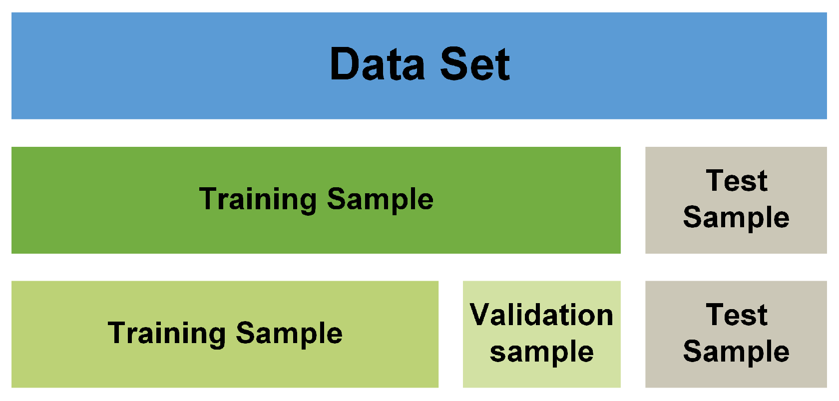
The algorithm receives the X variables (pictures) and makes a prediction (cat or dog). Knowing the value to predict, the algorithm can modify its behavior (its parameters) with each example it receives. The assumption is that over the course of iterations, the prediction error will decrease sufficiently so that the resulting model is able to predict the variable y, with new examples X that it has never observed. This is referred to as generalization. To evaluate the predictive ability of the model, the data are divided into two parts: the training sample and the validation sample. The model is trained on a sample of the data, and then, the validation set is sent to evaluate the average prediction errors of the model and to improve its performance by optimizing the hyperparameters. Once the hyperparameters have been optimized, the validation gives a first indicator of the model’s performance, indicating whether the model fits the data well. To know if a model has a good ability to generalize, the data are divided into two parts: the training sample and the test sample, as shown in Figure 4. The evaluation of the final model with the test sample gives a second performance indicator, on the ability to predict new data. In summary, the data are divided into three parts: the training sample, the validation sample, and the test sample. This procedure is called cross-validation.
Figure 5 shows two different curve fittings, where the coefficient of determination (R2) allows us to evaluate how well it fits the data, that is, the goodness of fit. The curve on the left has a coefficient of 0.71 and the one on the right of 0.85.
Although the curve on the right shows a better fit to the data, it is unlikely that this model will achieve good performance for prediction on new data. This phenomenon is often referred to as over-fitting. In the same way, a model that does not perform well on the training data might not have good predictive ability. This is what is called the bias/variance trade-off. By doing two evaluations of the performance of the model, it ensures that the model is well-balanced. Generally, supervised learning methods are divided into two families according to the variable to predict. First, there is classification, where the variable to predict is a discrete variable. Often, it is about predicting a class, a label, etc. Then, there is regression, where the variable to predict is a continuous variable. Figure 6 shows some well-known methods in supervised learning in regression and classification.

2.4.3. Unsupervised Learning

Unsupervised learning, as opposed to supervised learning, is the ML process where learning is done using unlabeled data [11]. The idea is to determine the relationships between variables without having a variable to predict. A classic use of this type of learning is data clustering. The objective of clustering is to categorize the data into subgroups that are determined by the similarity between the data [16]. Unsupervised learning is often used in big data where modeling can be very time-consuming, especially if all variables are included. Clustering, for example, can be used to reduce the number of variables in a dataset by grouping certain variables together based on common characteristics. A good example of clustering is the classification of animal species. By classifying animals by species (mammals, fish, birds, etc.), a large part of their characteristics is encapsulated in a single variable. The same kind of treatment is applied in supervised learning. Another class of unsupervised learning approach is dimensionality reduction. As the name implies, these methods take a dataset and reduce the dimensionality, i.e., the number of variables. For example, principal component analysis (PCA) consists of taking the data and trying to construct new variables by making changes to reference points (axes). The data are projected into a new simplified representation system (fewer variables) minimizing the loss of information. In a simplified way, the method consists in finding a line that minimizes the sum of the distances in a scatter plot, as in regression. Then, the points are projected (orthogonal projection) on this line, which becomes a new reference system, named the principal component. Figure 7 is adapted from the taxonomy developed in [16] to include the dimensionality reduction algorithm. It shows a classification of different unsupervised learning methods that are commonly used by practitioners.

2.4.4. Reinforcement Learning

Reinforcement learning is another type of machine learning algorithm. This type of learning is quite similar to the process studied in behavioral psychology, where one tries to induce behaviors through positive or negative reinforcement of the subject. These methods are frequently applied in robotics and in the field of video games, for instance [11]. In many cases, data are generated by the interaction of an intelligent agent (a machine) and its environment [17]. These data come from sensors, which bridge the gap between the physical and the computational, in the case of robots. From an algorithmic point of view, learning is done through these interactions with the environment and a penalty/reward function that guides the agent’s decisions. The goal of the intelligent agent is to maximize the rewards of its actions. As the agent makes decisions and receives feedback, it will become increasingly competent at performing the tasks it is trained to do [17]. Figure 8 presents a summary of the taxonomy of reinforcement learning algorithms developed by Zhang and Yu [18].

2.4.5. Deep Learning

Deep learning (DL) is a form of artificial intelligence. These methods take their name from the architecture of neural network algorithms. The neuron is the basic unit that makes up an artificial neural network (ANN), as demonstrated in Figure 9 [15]. The simple neuron, more formally the perceptron algorithm, takes a vector as input, as shown in the supervised learning example. These values are multiplied by their respective weights and aggregated by the input functions, then an activation function is applied to produce an output result.
A neural network, as its name suggests, is composed of successive layers of neurons, arranged in a network architecture. Deep learning occurs when a network has three or more layers [11]. Table 1 shows the three most common ANN architectures, along with their applications, as presented in [19].

2.4.6. Data Science

Data science is an emerging discipline. Its objective is to use the data to gain insight and turn those data into value for an organization [20]. General applications for data science include reporting, diagnosis, prediction, and recommendation. The field combines multiple other disciplines such as machine learning, data mining, statistics, data visualization, and predictive analytics [20]. Figure 10 presents the data science life cycle, which describes the general modeling process used by the practitioner. The first step of a data science project, like in applied research, is to define the problem and its objectives according to the business perspective and context. The data are then collected, cleaned, and prepared for modeling. Modeling is often performed using machine learning methods. The method and the performance metrics are selected according to the objectives defined and the type of problem at hand.

3. Machine Learning

3.1. Data Science Modeling Process

3.1.1. Data Acquisition

The first part of data-driven modeling is the data acquisition process. Data are generated automatically by sensing technology or by a technician through an ERP system, for example. The data are then loaded into a storage environment. The data can be structured and stored in a relational database or unstructured and stored in a data lake. Once the data are available in a stored environment, it can be prepared for modeling. Sometimes, relevant data may be stored across multiple sources and needs to be gathered for analytics.

3.1.2. Data Cleaning

Data quality is an important issue for data-driven modeling. For example, a case study applied to the reliability of mining equipment shows that raw data are often erroneous, lacking detail and accuracy, and, therefore, not suitable for decision-making. The study reveals that different fields of relational databases show errors in assigning maintenance tasks to the right subsystem, assigning codes to describe the type of work, associating the right type of maintenance (condition-based, preventive, corrective), etc. [22]. Cleaning must be performed so that the data are exploited to produce valuable insights for decision makers. In an ideal context, it is preferable that entry errors be prevented rather than corrected downstream. In fact, since the variance in data quality is greatly influenced by the user who enters it, it is essential to develop better management of the workers who interact with the database. Organizations must consider the effect of time pressure on data entry and provide feedback from supervisory staff to operators. In addition, it is necessary to encourage the participation of operators and to value their work toward data entry, in order to improve its quality [23]. Nonetheless, data scientists must ensure quality throughout the modeling and cleaning still needs to be performed. The data cleaning process involves the detection of errors and the removal or replacement in the dataset [24,25]. Figure 11 summarizes a methodology to quantify data quality (diagnostic) and manage its quality (correction) through a continuous process [24].
Cleaning of the dataset includes handling missing values, outliers, and bad data. The user can decide to correct the data with imputation techniques, get rid of the data, or leave it as it is [26]. To get rid of inadequate data, the user can either remove the entries (row) or delete a whole field (column), depending on the completeness (% of missing data) of a feature. For the imputation of missing values, the simplest methods are based on descriptive statistics. Good choices are central tendency measurement: for continuous variables, there is mean, mode, and median; for categorical variables, there is the most frequent value. Interpolation is often used for imputation in the case of a time series. Finally, some users may use machine learning techniques to replace missing values. The k-nearest neighbors’ algorithm (k-NN) and other regression methods are frequently used for this purpose [25].

3.1.3. Data Exploration

Once the data are gathered, data exploration or exploratory data analysis is done using graphical or statistical methods. Exploratory data analysis (EDA) is a practice that has been widely promoted by statistician John Wilder Tukey [27]. The idea behind EDA is to perform an initial examination of the data without any assumptions. Exploration is used to discover patterns or anomalies and then form a hypothesis on the data [27]. Common methods used in EDA are box plots, histograms, scatter plots, heatmaps, etc. The box plot, developed by Tukey, is used to represent graphically the minimum and maximum value, the median, and the quartile of a dataset. This graphic is very useful to detect outliers, in addition to showing the dispersion and skewness of a distribution. To graphically observe the shape of a distribution, the preferred representation is the histogram, which makes it an excellent tool for EDA. The scatter plot is used to plot the point of two variables as coordinates. Heatmaps, in the context of data analysis, are used to plot covariates against each other’s and demonstrate the relationships, often using a correlation matrix. Data exploration generally starts at the beginning of the modeling project but is used throughout the entire process. For example, a box plot is a good method for detecting outliers and can help with data cleaning. Additionally, heatmaps are a good starting point for selecting or eliminating features in the step of feature engineering.

3.1.4. Feature Engineering

When dealing with real-world data, there can be hundreds of features, and it is necessary to select the most relevant one from a dataset. Feature engineering is a process that includes feature selection, feature transformation, feature creation/feature construction, and feature extraction. The goal of this process is to reduce the size of the dataset by selecting and transforming features to optimize the learning of a model. Feature selection is the process of selecting the most relevant variables to perform modeling. Some variables may be irrelevant to the phenomenon studied, but some variables that are relevant may have unwanted effects on the model. For example, a feature may be redundant since it is highly correlated with another explanatory variable. When dealing with lots of variables, it is important to select the feature that will better explain the phenomenon without being too computationally intensive. Correlation coefficients (Pearson) and heatmaps are good methods for feature selection, as well as analysis of variance (ANOVA) tests and hypothesis testing. Sometimes, machine learning algorithms such as tree-based models (random forest (RF), decision tree (DT), etc.) are used in feature selection [28]. Feature transformation includes feature normalization and linearization. Feature normalization consists of scaling the values of a feature so that all features have the same contribution to the model. Many ML techniques use Euclidean distances to compute the distance between points. If the numerical features are not proportional, the estimation might be biased towards the largest variables [25,26]. Linearization is a technique to transform the points of a distribution so that they can be represented by a linear function. This method is widely used in reliability for the exponential distribution. With a logarithmic transformation, a curve fitting of the data gives the equation of exponential or Weibull distribution, for example [9]. Feature extraction is associated with dimensionality reduction techniques. The concept is to reduce the number of features by combining features with a linear projection in a lower dimensionality space. Feature creation or feature construction consists of using existing variables to create new features that are more appropriate for modeling. Examples of feature creation include encoding techniques (one-hot encoding, label encoding) and binning. Features can also be created with clustering methods, where the new variables represent groups of points with similarity [16].

3.1.5. Model Conception

According to what has been described in the previous sections, machine learning methods are used well before the design of the asset model. However, it is during the design of this model that the methods diverge between RAMS and PHM. Although some techniques are similar, the purpose of the models and their context is different, as presented in Section 4 and Section 5. Figure 10 refers to predictive modeling, but it can be interpreted in a more general context as modeling of any kind (classification, prediction, clustering, curve fitting, etc.). In the case of a machine learning model, the method consists of training the model and validating its performance, for example, by cross-validation, and then using it to generate new knowledge from data. The same process applies to statistical modeling: the model is fitted to the data, and then the goodness of fit is evaluated with different performance metrics.

4. ML Applications Analysis

This section of the paper aims to analyze the literature on reliability engineering, particularly machine learning methods that have been used by practitioners. An analysis of applications in RAMS and PHM will give a clear picture of why and how ML modeling is used and identify gaps between theoretical applications and industry use cases.

4.1. Results

4.1.1. Execution and Filtering of Results

The keyword search on the two databases available on EBSCO gave hundreds of results. To reduce the number of publications, the search will focus on articles from the last 5 years that deal with either RAMS or PHM. Additionally, the complete article must be available for download, as it is important to review the work. The EBSCO filter tool allows making these selections quickly, especially with the publication date filter, the source type (academic journals), and the help of the thesaurus, to select publication by subject. Finally, of these results, only a few articles correspond to the subject in question, and the last filtering is done manually. Table 2 presents the different selection and exclusion rules, as well as the number of publications that match this criterion.

4.1.2. Applications Analysis

As mentioned earlier, RAMS is a framework for evaluating and optimizing the performance of a system, focusing on the general characteristics of a population, while PHM is a more proactive approach that involves continuously monitoring a system to predict and prevent potential failures. We classified each article and its application according to these definitions. Figure 12 shows the distribution of publications each year, by the subject of application. We notice that the number of publications per subject is quite similar for RAMS and PHM, with small variations over the years. We also notice that there is a strong increase in the overall number of publications in 2020, which corresponds to the outbreak of the pandemic, and then a significant decrease the following year.

4.1.3. Machine Learning Methods Review

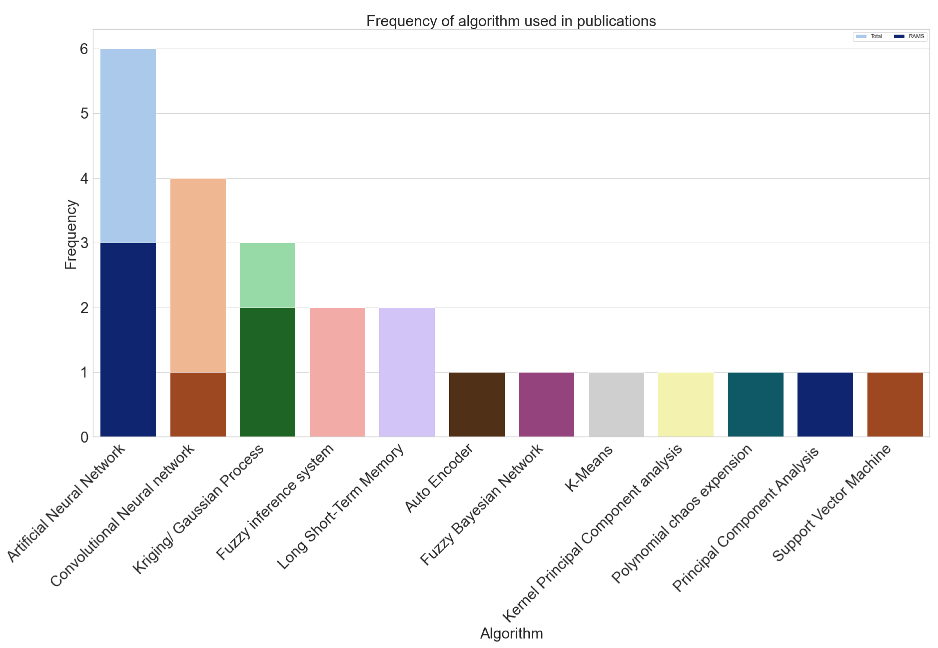
Figure 13 shows the different machine learning methods that were used in the articles. The artificial neural network is the most used method of all, being used in more than 30% of the studies. Furthermore, considering the different architectures of neural networks (convolutional networks, auto-encoders, and recurrent neural networks (RNNs) of type LSTM (long-short-term memory)), more than half of the methods are deep learning. Figure 13 shows the total number of uses of the algorithm used in RAMS versus in total. Although deep learning methods are the most popular, the figure demonstrates that they are generally more used in PHM research than in RAMS. When examining publication objectives in prognostics, it seems that the research is more focused either on remaining useful life (RUL) estimation or online monitoring and diagnostics. Both applications require a large amount of data to build a supervised prediction model, so it is not surprising that deep learning is the preferred ML approach. Furthermore, recurrent neural network methods such as LSTM can account for time dependencies because of their architecture, which contains feedback connections between layers, making it an excellent solution for RUL estimation. In RAMS, ML methods and modeling objectives are more diverse. For example, [29] tested deep learning approaches to solve the problem of stochastic flow manufacturing networks to predict the overall reliability of a manufacturing production line. Another study uses a support vector machine (SVM)-based algorithm to solve an optimization problem of structure reliability. Other RAMS applications apply machine learning to simulate possible scenarios and evaluate system reliability [30,31]. The vast majority of techniques, for both RAMS and PHM, are supervised learning methods; some studies have also used transfer learning and self-supervised learning. Table 3 shows in which articles each of the techniques were used.

4.1.4. Datasets and Systems under Study

In this section, we present the different types of datasets that are used in the literature, as well as the different systems that these data come from.
As shown in Figure 14, 47% of the studies use simulated data or data that are generated randomly by theoretical mathematical functions. Then, 29% of the publications used public datasets; these data are freely available to the public for different uses. A large proportion of public datasets are actual operational data. However, their treatment is simplified compared to a real case study, and their use is mainly intended to test and compare new approaches with existing methods. Many organizations make their data available to the public on a platform such as Google Dataset Search or Kaggle. For example, in [32], they used data from NASA’s Turbofan engine degradation simulation [33] to compare the new RNN architecture for the estimation of the remaining useful life. In [34], they used NASA’s experimental data on lithium-ion batteries to test a new CNN-LSTM architecture to improve the precision of the prediction of remaining useful life [35]. Less than a quarter of the study are interested in the analysis of industrial case studies (6%) through experimental testing and operational data (18%).
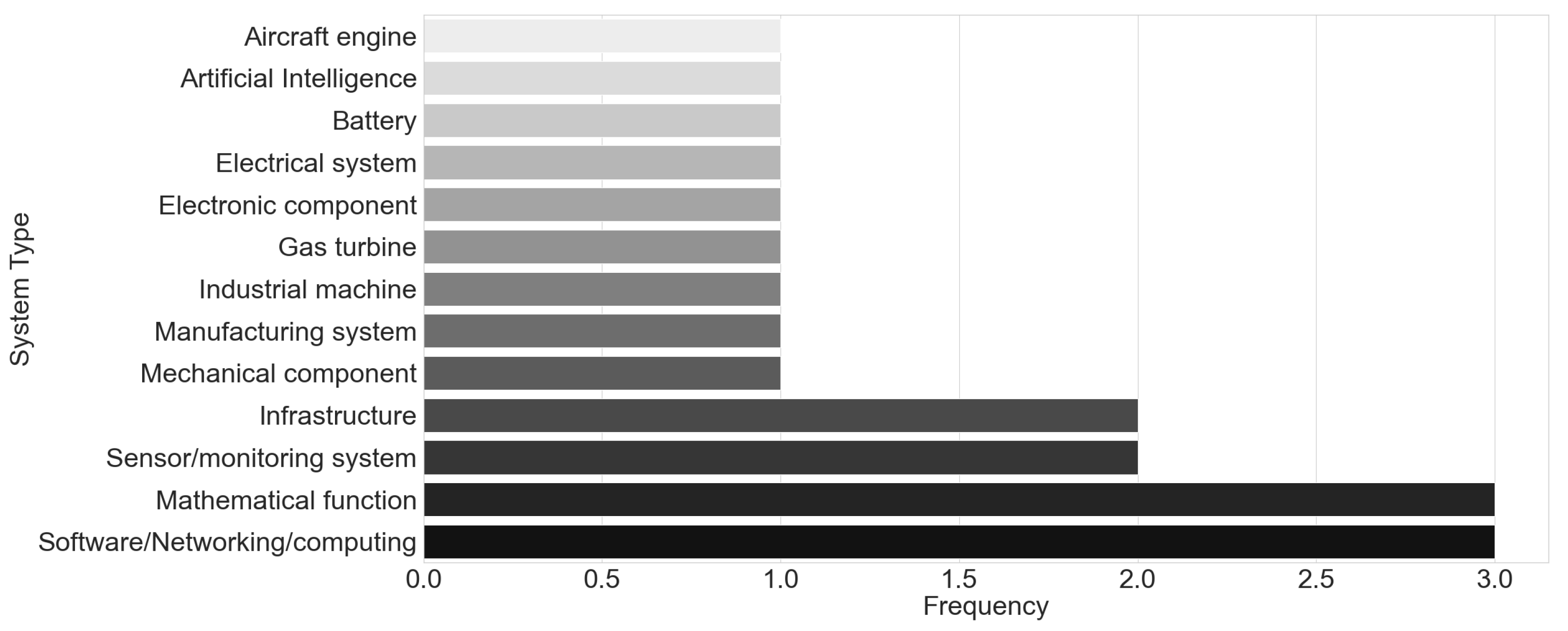
The types of systems studied are very diverse, as shown in Figure 15. The reliability of computer networks and software is a subject that has been studied extensively, and this is reflected in the graph. As shown in Figure 14, theoretical studies using various mathematical functions are very popular, instead of using real-life systems. Another topic that is relatively popular is the reliability of the monitoring and sensing systems themselves. Indeed, it is important to consider the possibility that monitoring systems produce misleading signals and themselves suffer from failures to improve decision-making in an organization.

4.2. Related Works

The systematic review presented in the previous section provides a comprehensive and reliable overview of the evidence on the topic of machine learning applied to reliability. However, the review is based on two databases, potentially excluding interesting articles on the subject. Therefore, this section aims to supplement the review by presenting some additional applications as well as programming tools for practitioners. To begin with, in [36], the authors present an agent-based modeling method for simulation to study the balancing of smart grids. The objective is to use this model to test the effect of balancing on electrical and telecommunications networks, among others. In [37], an attempt is made to develop a model to predict failures, taking into account several covariates while considering possible interactions. An approach to combining a neural network, specifically a single-layer perceptron, with the method of general renewal Weibull process for curve fitting is presented. Finally, the approach is tested through a case study on solar power plants and presented, particularly by analyzing the reliability of thermal pumps. In [38], a structure and method are developed to reduce the dimensionality of asset lifecycle data while minimizing information losses. This PHM application also focuses on feature engineering by introducing a data transformation method to prepare ML models for predictive maintenance. The proposed framework appears promising, but the article lacks an application to demonstrate the applicability and relevance of the method. On the other hand, in [39], a similar methodology is attempted in a case study in a machining center. The authors use a supervised learning technique of feature selection: minimum redundancy maximum relevance. The analyses demonstrate that the method has eliminated about ten redundant variables. Then, a model is built from historical data, and the results are used to produce a monitoring tool for enterprise management. A rule-based model is then used for predictive maintenance. In [40], a preventive maintenance model is developed to improve policies, in addition to presenting a cloud architecture for a predictive maintenance and corrective maintenance program with real-time detection. A case study is presented to analyze the residual life of equipment in a machining center. An artificial neural network is trained from historical data and then used for real-time monitoring. The article [41] presents a reliability study in the context of a semiconductor manufacturer. The objective is to present a model that can learn and associate indicators with potential failures and determine rules or patterns of indicators or critical areas. They use Bayesian networks to determine probability distributions in the learning phase, then use the resulting network to learn patterns leading to failure. The results suggest that the model could be extended to real-time prediction applications. A growing area of research in reliability is natural language processing (NLP), particularly for leveraging historical data in the form of free text. In [42], the authors discuss the need to develop a new methodology, technical language processing, to adapt NLP to the context of short technical text analysis. Indeed, traditional NLP tools are not suitable for processing technical language contained in engineering databases; the texts are generally short and contain abbreviations or domain-specific language for example. The article proposes a new framework to address the reality of short texts contained in maintenance work orders. In [43], a case study is presented for the classification of maintenance data in a manufacturing company. CamemBERT, a pre-trained transformer architecture, is used for French language processing. In [44], a classification model is developed based on a pre-trained model for reclassifying maintenance orders in the context of an electrical utility. Some reviews of the literature also present interesting perspectives on reliability. The authors of [45] propose a summary of the literature on the application of the k-out-of-n: G system method for evaluating the reliability of the system. This method aims to analyze the reliability of a system consisting of n components, which can operate as long as k components function. This method is particularly useful in the analysis of complex systems. Finally, Ref. [46] provides a summary of the literature on statistical techniques in reliability, particularly for predicting failures and applications of heavy equipment in the mining industry. In addition, they propose to compare traditional methods with machine learning methods by analyzing case studies presented in the literature.
Table 4 presents various programming tools, and Python libraries, which are widely used by the scientific community and in the field of RAMS engineering. In particular, the Reliability [47], Lifelines [48], and Scikit-survival [49] libraries allow for several statistical analyses relevant to RAMS, including parametric analyses with known distributions such as Weibull, Gamma, and Exponential, as well as survival analyses. The ProgPy [50] library is a recently developed library by NASA for PHM applications. The statsmodels [51] library is a general statistical library, while Scikit-Learn [52] is a general ML library containing a multitude of methods. TensorFlow [53] and Keras [54] are among the most widely used libraries for deep learning development. Finally, NLTK [55] and Spacy [52] are two open-access libraries offering easy and quick integration of tools for natural language processing.

4.3. Discussion

This section allows us to make several observations regarding the use of machine learning in the field of reliability. Although this review only lists the results of a few databases, it still allows us to have an insightful overview of the situation. The number of publications found on the subject has been quite low for the last 5 years (19 articles), although there is a growing trend for artificial intelligence applications. When you look at the data sources, this gives a hint as to why there are no more publications in the field. Indeed, most of the publications apply ML to fictive data, in particular with the aim of developing new methodologies. Case studies are quite rare: less than a quarter of publications. The difficulty to obtain good-quality operational data is probably part of the problem. However, the development of new methodologies can be expected to lead to case studies on real data. The data used in reliability are sometimes difficult to exploit, given the complexity of the data (manually entered data, free text fields, etc.). Moreover, machine learning requires a large amount of data, which means that it is necessary to have a large database of historical maintenance work, which is a considerable constraint in itself. Given these factors, this also justifies why deep learning approaches are generally preferred in the field.

Future Work

This research introduces the concepts of machine learning and reliability engineering. Learning these concepts is essential to start applying advanced techniques in the industry. Although the general concepts may be perceived as well mastered by the community, the systematic review shows that there are still few applications that are made in real industrial contexts. With the rapid development of Industry 4.0 and the various enablers, it is becoming clear that it is only a matter of time before these methods spread throughout the industry. To do so, the research community needs to prove that machine learning can be applied to real, often imperfect data.

5. Conclusions

The field of reliability engineering has seen tremendous growth in recent years due to advancements in data acquisition and processing technologies. However, the integration of artificial intelligence (AI) techniques into the domain remains a complex task. The goal of this publication is to summarize the basic techniques used in reliability and machine learning in order to demonstrate how they can be applied in an industrial context. The first sections focused on providing a summary of the techniques by presenting the basics of modeling and statistical techniques, followed by a comprehensive overview of machine learning, artificial intelligence, and data science. These sections provided a solid foundation to understand the different types of techniques used for modeling. Then a systematic review of machine learning applied in reliability engineering was presented. An analysis was done by linking the analysis domain (RAMS or PHM), the type of algorithm, and the type of system in which it is involved. Furthermore, the review compared the types of data used, whether synthetic or operational. Finally, an overview of related works was presented, introducing different machine learning applications and tools used in real-world applications. This provided a good overview of different use cases of machine learning for reliability engineering.
The findings of this review suggest that machine learning techniques are still not widely used in the reliability engineering field. The results also showed that most of the studies did not use operational data as input for their models, but rather used synthetic data or publicly available datasets. In addition, deep learning techniques (deep neural network) are the most widely used machine learning method in reliability.
In conclusion, the application of machine learning techniques in RAMS and PHM gives new opportunities for researchers and practitioners to optimize the decision-making processes and improve the reliability and performance of systems. This work provides a good foundation for researchers with an understanding of the field of machine learning applied to reliability engineering. However, there is still great difficulty in working with operational data, opening the way for applied research in data mining and natural language processing, particularly for the analysis of maintenance data.

Author Contributions

Conceptualization, M.P. and G.A.-N.; methodology, M.P. and G.A.-N.; validation, G.A.-N.; writing—original draft preparation, M.P.; writing—review and editing, M.P. and G.A.-N.; supervision, G.A.-N.; project administration, G.A.-N. All authors have read and agreed to the published version of the manuscript.

Funding

This research received no external funding.

Institutional Review Board Statement

Not applicable.

Informed Consent Statement

Not applicable.

Data Availability Statement

Data sharing is not applicable.

Acknowledgments

This research was supported by Hydro-Québec, the Natural Sciences and Engineering Research Council of Canada (NSERC), and the Université du Québec à Trois-Rivières through the Hydro-Québec Asset Management Research Chair.

Conflicts of Interest

The authors declare no conflict of interest.

References

  1. Iafrate, F. Artificial Intelligence and Big Data: The Birth of a New Intelligence; John Wiley & Sons: Hoboken, NJ, USA, 2018. [Google Scholar]
  2. Sage, M.; Zhao, Y.F. Is Machine Learning Suitable to Improve My Process? McGill University: Montreal, QC, Canada, 2020. [Google Scholar]
  3. Pecht, M.; Kumar, S. Data analysis approach for system reliability, diagnostics and prognostics. In Proceedings of the Pan Pacific Microelectronics Symposium, Kauai, HI, USA, 22–24 January 2008; Volume 795, pp. 1–9. [Google Scholar]
  4. Dersin, P. Prognostics & Health Management for Railways: Experience, Opportunities, Challenges. In Proceedings of the Applied Reliability and Durability Conference, Amsterdam, The Netherlands, 23–25 June 2020. [Google Scholar]
  5. Stillman, G.A.; Kaiser, G.; Blum, W.; Brown, J.P. Teaching Mathematical Modelling: Connecting to Research and Practice; Springer Science & Business Media: Berlin/Heidelberg, Germany, 2013. [Google Scholar]
  6. Stender, P. The use of heuristic strategies in modelling activities. ZDM 2018, 50, 315–326. [Google Scholar] [CrossRef] [Green Version]
  7. Biau, G.; Herzlich, M.; Droniou, J. Mathematiques et Statistique pour les Sciences de la Nature: Modeliser, Comprendre et Appliquer; Collection Enseignement sup.; Mathematiques, EDP Sciences: Les Ulis, France, 2010. [Google Scholar]
  8. Hicks, C.R.; Turner, K.V. Fundamental Concepts in the Design of Experiments, 5th ed.; Oxford University Press: New York, NY, USA, 1999. [Google Scholar]
  9. Lewis, E.E. Introduction to Reliability Engineering, 2nd ed.; Reliability Engineering; J. Wiley and Sons: New York, NY, USA, 1996; 435p. [Google Scholar]
  10. Van Harmelen, F.; Lifschitz, V.; Porter, B. Handbook of Knowledge Representation; Elsevier: Amsterdam, The Netherlands, 2008. [Google Scholar]
  11. Hurwitz, J.; Kirsch, D. Machine Learning for Dummies; John Wiley & Sons, Inc.: Hoboken, NJ, USA, 2018. [Google Scholar]
  12. Haenlein, M.; Kaplan, A. A brief history of artificial intelligence: On the past, present, and future of artificial intelligence. Calif. Manag. Rev. 2019, 61, 5–14. [Google Scholar] [CrossRef]
  13. Press, G. A Very Short History of Artificial Intelligence (AI). Forbes Magazine, 30 December 2016. [Google Scholar]
  14. IBM. Big DATA for the Intelligence Community; Report; IBM: Armonk, NJ, USA, 2013. [Google Scholar]
  15. Russell, S.; Norvig, P. Artificial Intelligence: A Modern Approach; Pearson Education, Inc.: London, UK, 2002. [Google Scholar]
  16. Fahad, A.; Alshatri, N.; Tari, Z.; Alamri, A.; Khalil, I.; Zomaya, A.Y.; Foufou, S.; Bouras, A. A survey of clustering algorithms for big data: Taxonomy and empirical analysis. IEEE Trans. Emerg. Top. Comput. 2014, 2, 267–279. [Google Scholar] [CrossRef]
  17. Akalin, N.; Loutfi, A. Reinforcement learning approaches in social robotics. Sensors 2021, 21, 1292. [Google Scholar] [CrossRef]
  18. Zhang, H.; Yu, T. Taxonomy of reinforcement learning algorithms. In Deep Reinforcement Learning; Springer: Singapore, 2020; pp. 125–133. [Google Scholar]
  19. Zhu, N.; Liu, X.; Liu, Z.; Hu, K.; Wang, Y.; Tan, J.; Huang, M.; Zhu, Q.; Ji, X.; Jiang, Y. Deep learning for smart agriculture: Concepts, tools, applications, and opportunities. Int. J. Agric. Biol. Eng. 2018, 11, 32–44. [Google Scholar] [CrossRef]
  20. Van der Aalst, W.M. Process Mining: Data Science in Action; Springer: Berlin/Heidelberg, Germany, 2016. [Google Scholar]
  21. Agarwal, S. Understanding the Data Science Lifecycle. 2018. Available online: https://www.sudeep.co/data-science/2018/02/09/Understanding-the-Data-Science-Lifecycle.html (accessed on 26 March 2023).
  22. Ho, M.; Hodkiewicz, M.R.; Pun, C.F.; Petchey, J.; Li, Z. Asset Data Quality—A Case Study on Mobile Mining Assets; Springer: Berlin/Heidelberg, Germany, 2015; pp. 335–349. [Google Scholar]
  23. Murphy, G.D. Improving the quality of manually acquired data: Applying the theory of planned behaviour to data quality. Reliab. Eng. Syst. Saf. 2009, 94, 1881–1886. [Google Scholar] [CrossRef] [Green Version]
  24. Berti-Équille, L. Qualité des données. In Techniques de l’Ingénieur Bases de Données; Base Documentaire: TIB309DUO; Technique de l’ingénieur: Saint-Denis, France, 2018. [Google Scholar]
  25. Pecht, M.G.; Kang, M. Prognostics and Health Management of Electronics; Wiley: Hoboken, NJ, USA, 2018. [Google Scholar]
  26. Grus, J. Data Science from Scratch: First Principles with Python; O’Reilly Media: Sebastopol, CA, USA, 2019. [Google Scholar]
  27. Martinez, W.L.; Martinez, A.R.; Solka, J.L. Exploratory Data Analysis with MATLAB®; Chapman and Hall/CRC: Boca Raton, FL, USA, 2017. [Google Scholar]
  28. Ozdemir, S.; Susarla, D. Feature Engineering Made Easy: Identify Unique Features from Your Dataset in Order to Build Powerful Machine Learning Systems; Packt Publishing Ltd.: Birmingham, UK, 2018. [Google Scholar]
  29. Yi-Fan, C.; Yi-Kuei, L.; Cheng-Fu, H. Using Deep Neural Networks to Evaluate the System Reliability of Manufacturing Networks. Int. J. Perform. Eng. 2021, 17, 600–608. [Google Scholar] [CrossRef]
  30. Nabian, M.A.; Meidani, H. Deep Learning for Accelerated Seismic Reliability Analysis of Transportation Networks. Comput.-Aided Civ. Infrastruct. Eng. 2018, 33, 443–458. [Google Scholar] [CrossRef] [Green Version]
  31. Wei-Ting, L.I.N.; Hsiang-Yun, C.; Chia-Lin, Y.; Meng-Yao, L.I.N.; Kai, L.; Han-Wen, H.U.; Hung-Sheng, C.; Hsiang-Pang, L.I.; Meng-Fan, C.; Yen-Ting, T.; et al. DL-RSIM: A Reliability and Deployment Strategy Simulation Framework for ReRAM-based CNN Accelerators. ACM Trans. Embed. Comput. Syst. 2022, 21, 1–29. [Google Scholar] [CrossRef]
  32. Gritsyuk, K.M.; Gritsyuk, V.I. Convolutional And Long Short-Term Memory Neural Networks Based Models For Remaining Useful Life Prediction. Int. J. Inf. Technol. Secur. 2022, 14, 61–76. [Google Scholar]
  33. Saxena, A.; Goebel, K. Turbofan Engine Degradation Simulation Data Set; NASA: Washington, DC, USA, 2008. [Google Scholar]
  34. Kara, A. A data-driven approach based on deep neural networks for lithium-ion battery prognostics. Neural Comput. Appl. 2021, 33, 13525–13538. [Google Scholar] [CrossRef]
  35. Saha, B.; Goebel, K. Battery Data Set. In NASA AMES Prognostics Data Repository; NASA: Washington, DC, USA, 2007. [Google Scholar]
  36. Kilkki, O.; Kangasrääsiö, A.; Nikkilä, R.; Alahäivälä, A.; Seilonen, I. Agent-based modeling and simulation of a smart grid: A case study of communication effects on frequency control. Eng. Appl. Artif. Intell. 2014, 33, 91–98. [Google Scholar] [CrossRef]
  37. Gomez Fernandez, J.F.; Olivencia, F.; Ferrero, J.; Marquez, A.C.; Garcia, G.C. Analysis of dynamic reliability surveillance: A case study. IMA J. Manag. Math. 2018, 29, 53–67. [Google Scholar] [CrossRef] [Green Version]
  38. Aremu, O.O.; Palau, A.S.; Parlikad, A.K.; Hyland-Wood, D.; McAree, P.R. Structuring Data for Intelligent Predictive Maintenance in Asset Management. IFAC-PapersOnLine 2018, 51, 514–519. [Google Scholar] [CrossRef]
  39. Fernandes, M.; Canito, A.; Bolón-Canedo, V.; Conceição, L.; Praça, I.; Marreiros, G. Data analysis and feature selection for predictive maintenance: A case-study in the metallurgic industry. Int. J. Inf. Manag. 2019, 46, 252–262. [Google Scholar] [CrossRef]
  40. Wan, J.; Tang, S.; Li, D.; Wang, S.; Liu, C.; Abbas, H.; Vasilakos, A.V. A manufacturing big data solution for active preventive maintenance. IEEE Trans. Ind. Inform. 2017, 13, 2039–2047. [Google Scholar] [CrossRef]
  41. Abu-Samah, A.; Shahzad, M.K.; Zamai, E.; Said, A.B. Failure Prediction Methodology for Improved Proactive Maintenance using Bayesian Approach. IFAC-PapersOnLine 2015, 48, 844–851. [Google Scholar] [CrossRef]
  42. Brundage, M.P.; Sexton, T.; Hodkiewicz, M.; Dima, A.; Lukens, S. Technical language processing: Unlocking maintenance knowledge. Manuf. Lett. 2021, 27, 42–46. [Google Scholar] [CrossRef]
  43. Naqvi, S.M.R.; Varnier, C.; Nicod, J.M.; Zerhouni, N.; Ghufran, M. Leveraging free-form text in maintenance logs through bert transfer learning. In Proceedings of the Progresses in Artificial Intelligence & Robotics: Algorithms & Applications: Proceedings of 3rd International Conference on Deep Learning, Artificial Intelligence and Robotics, (ICDLAIR) 2021; Springer: Berlin/Heidelberg, Germany, 2022; pp. 63–75. [Google Scholar]
  44. Payette, M.; Abdul-Nour, G.; Meango, T.J.M.; Côté, A. Improving Maintenance Data Quality: Application of Natural Language Processing to Asset Management. In 16th WCEAM Proceedings; Springer: Berlin/Heidelberg, Germany, 2023; pp. 582–589. [Google Scholar]
  45. Krishnan, R. Reliability Analysis of k-out-of-n: G System: A Short Review. Int. J. Eng. Appl. Sci. (IJEAS) 2020, 7, 21–24. [Google Scholar] [CrossRef]
  46. Odeyar, P.; Apel, D.B.; Hall, R.; Zon, B.; Skrzypkowski, K. A Review of Reliability and Fault Analysis Methods for Heavy Equipment and Their Components Used in Mining. Energies 2022, 15, 6263. [Google Scholar] [CrossRef]
  47. Reid, M. Reliability—A Python Library for Reliability Engineering, Version 0.5. 2020. Available online: https://zenodo.org/record/3938000#.ZC4xK3ZBxPY(accessed on 26 March 2023).
  48. Davidson-Pilon, C. Lifelines: Survival analysis in Python. J. Open Source Softw. 2019, 4, 1317. [Google Scholar] [CrossRef] [Green Version]
  49. Pölsterl, S. Scikit-survival: A Library for Time-to-Event Analysis Built on Top of scikit-learn. J. Mach. Learn. Res. 2020, 21, 1–6. [Google Scholar]
  50. Teubert, C.; Jarvis, K.; Corbetta, M.; Kulkarni, C.; Daigle, M. ProgPy Python Prognostics Packages. 2022. Available online: https://nasa.github.io/progpy (accessed on 26 March 2023).
  51. Seabold, S.; Perktold, J. statsmodels: Econometric and statistical modeling with python. In Proceedings of the 9th Python in Science Conference, Austin, TX, USA, 28 June–3 July 2010. [Google Scholar]
  52. Pedregosa, F.; Varoquaux, G.; Gramfort, A.; Michel, V.; Thirion, B.; Grisel, O.; Blondel, M.; Prettenhofer, P.; Weiss, R.; Dubourg, V.; et al. Scikit-learn: Machine Learning in Python. J. Mach. Learn. Res. 2011, 12, 2825–2830. [Google Scholar]
  53. Abadi, M.; Agarwal, A.; Barham, P.; Brevdo, E.; Chen, Z.; Citro, C.; Corrado, G.S.; Davis, A.; Dean, J.; Devin, M.; et al. TensorFlow: Large-Scale Machine Learning on Heterogeneous Systems. 2015. Available online: www.tensorflow.org (accessed on 10 March 2023).
  54. Chollet, F. Keras. 2015. Available online: https://keras.io (accessed on 10 March 2023).
  55. Bird, S.; Klein, E.; Loper, E. Natural Language Processing with Python: Analyzing Text with the Natural Language Toolkit; O’Reilly Media, Inc.: Sebastopol, CA, USA, 2009. [Google Scholar]
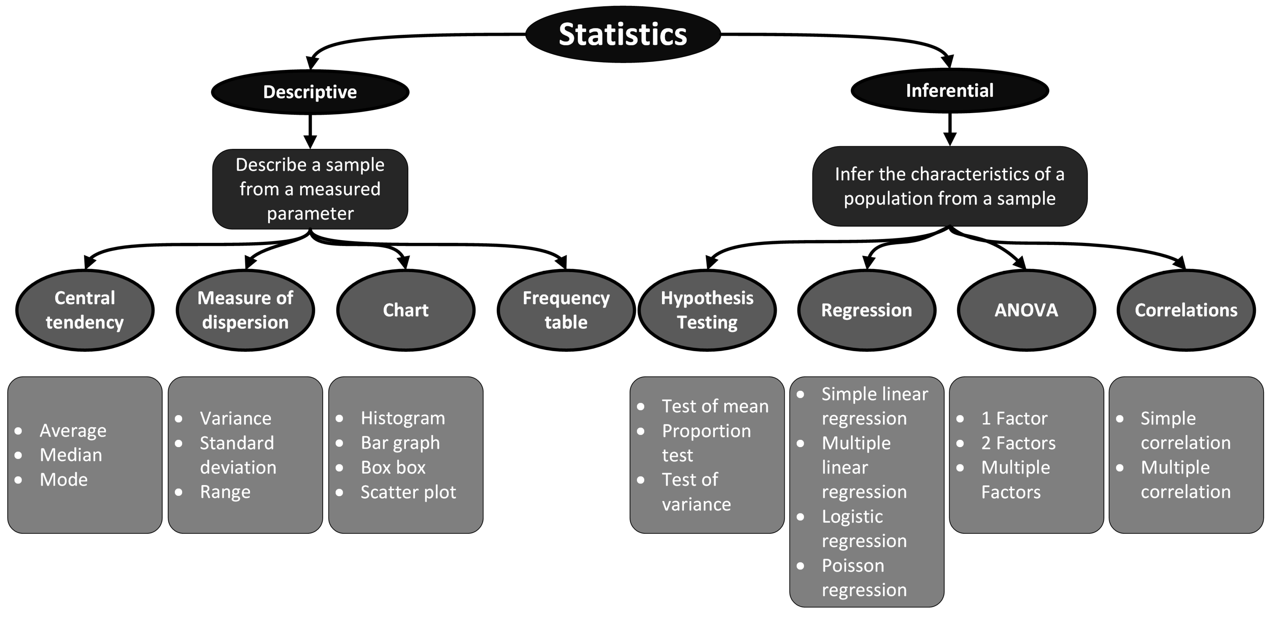
Figure 1. Common statistical modeling techniques.
Sustainability 15 06270 g001
Figure 2. Artificial intelligence development.
Sustainability 15 06270 g002
Figure 3. Example of supervised learning.
Sustainability 15 06270 g003
Figure 4. Example of data sampling for SL.
Sustainability 15 06270 g004
Figure 5. Example of curve fitting.
Sustainability 15 06270 g005
Figure 6. Supervised learning approaches and algorithm.
Sustainability 15 06270 g006
Figure 7. Unsupervised learning algorithm.
Sustainability 15 06270 g007
Figure 8. Taxonomy of reinforcement learning algorithm.
Sustainability 15 06270 g008
Figure 9. A simple mathematical model for a neuron.
Sustainability 15 06270 g009
Figure 10. Data science life cycle adapted from [21].
Sustainability 15 06270 g010
Figure 11. Virtuous circle for data quality management adapted from [24].
Sustainability 15 06270 g011
Figure 12. Publications per year by topic.
Sustainability 15 06270 g012
Figure 13. Frequency of use of ML algorithms by topic.
Sustainability 15 06270 g013
Figure 14. Pie chart of types of data sources.
Sustainability 15 06270 g014
Figure 15. Types of systems under study.
Sustainability 15 06270 g015
Table 1. ANN architectures and applications.
TypeStructureApplications
Artificial Neural NetworkInput layerClassification
Hidden layersRegression
Output layerPattern recognition
Convolutional Neural NetworkInput layer
Convolution layersNatural language processing
Pooling layerImage processing
Fully connected layer
Output layer
Recurrent Neural NetworkInput layerTime series analysis
Hidden layersSentiment Analysis
Output layerNatural language processing
Table 2. Results filtering.
RuleNumbers of Publications
Keywords547
From 2017 to 2023362
Works not related to reliability engineering253
English or French only251
Full-text available38
Peer-reviewed34
Hand-selected19
Table 3. Algorithms associated with reviewed articles.
TitleAuthorsData TypeAlgorithm
Effective software fault localization using predicted execution resultsGao, Wong et al., 2017OperationalK-Means
An Intelligent Reliability Assessment technique for Bipolar Junction Transistor using Artificial Intelligence TechniquesBhargava and Handa 2018Experimental testingArtificial Neural Network, Fuzzy Inference System
Active fault tolerant control based on a neuro fuzzy inference system applied to a two shafts gas turbineHadroug, Hafaifa et al., 2018OperationalArtificial Neural Network, Fuzzy inference system
Deep Learning for Accelerated Seismic Reliability Analysis of Transportation NetworksNabian and Meidani 2018Simulated/
Generated randomly
Artificial Neural Network
Gaussian Process-Based Response Surface Method for Slope Reliability AnalysisHu, Su et al., 2019Simulated/
Generated randomly
Kriging/Gaussian Process
Fault diagnosis of multi-state gas monitoring network based on fuzzy Bayesian netXue, Li et al., 2019OperationalFuzzy Bayesian Network
Active learning polynomial chaos expansion for reliability analysis by maximizing expected indicator function prediction errorCheng and Lu 2020Simulated/
Generated randomly
Polynomial Chaos Expansion, Kriging/Gaussian Process
A Reliability Management System for Network Systems using Deep Learning and Model Driven ApproachesMin, Jiasheng et al., 2020Simulated/
Generated randomly
Artificial Neural Network
Integration of Dimension Reduction and Uncertainty Quantification in Designing Stretchable Strain Gauge SensorSungkun, Gorguluarslan et al., 2020Simulated/
Generated randomly
Auto Encoder, Artificial Neural Network, Principal Component Analysis
Data-driven prognostic method based on self-supervised learning approaches for fault detectionWang, Qiao et al., 2020Public datasetKernel Principal Component Analysis
Transfer Learning Strategies for Deep Learning-based PHM AlgorithmsYang, Zhang et al., 2020Public datasetConvolutional Neural Network
Bounds approximation of limit-state surface based on active learning Kriging model with truncated candidate region for random-interval hybrid reliability analysisYang, Wang et al., 2020Simulated/
Generated randomly
Kriging/Gaussian Process
A data-driven approach based on deep neural networks for lithium-ion battery prognosticsKara 2021Public datasetConvolutional Neural Network, Long Short-Term Memory
Using Deep Neural Networks to Evaluate the System Reliability of Manufacturing NetworksYi-Fan, Yi-Kuei et al., 2021Simulated/
Generated randomly
Artificial Neural Network
Convolutional And Long Short-Term Memory Neural Networks Based Models For Remaining Useful Life PredictionGritsyuk and Gritsyuk 2022Public datasetConvolutional Neural Network, Long Short-Term Memory
DL-RSIM: A Reliability and Deployment Strategy Simulation Framework for ReRAM-based CNN AcceleratorsWei-Ting, Hsiang-Yun et al., 2022Public datasetConvolutional Neural Network
A Novel Support-Vector-Machine-Based Grasshopper Optimization Algorithm for Structural Reliability AnalysisYang, Sun et al., 2022Simulated/
Generated randomly
Support Vector Machine
Table 4. Python libraries for reliability engineering.
Library NameApplicationLibrary Function
ReliabilityReliability and Survival AnalysisParametric Reliability Models (Weibull, Exponential, Lognormal, etc.), Non-Parametric Models (Kaplan–Meier, Nelson–Aalen, etc.), Accelerated Life Testing
LifelinesSurvival AnalysisCox Proportional Hazard Model, Kaplan–Meier Estimator, Parametric Survival Models
Scikit-survivalSurvival AnalysisSurvival Tree, Ensemble Model for Survival Analysis, Cox Proportional Hazard Model, Kaplan–Meier Estimator
ProgPy Python Prognostics PackagesPrognostics
StatsmodelsStatisticsLinear Regression, Generalized Linear Model, ANOVA
Scikit-LearnMachine LearningClassification, Regressions, Clustering, Cross-Validation/Model Selection Methods
TensorFlowDeep LearningArtificial Neural Network, Recurrent Neural Network, Convolutional Neural Network
KerasDeep LearningHigh-level API built on top of Tensor Flow for easy use
NLTKNatural Language ProcessingTokenization, Sentiment Analysis, Stemming, Part-of-Speech Tagging
SpacyNatural Language ProcessingText Classifier, Transformer Models, Custom Trainable Pipeline, Named Entity Recognition
Disclaimer/Publisher’s Note: The statements, opinions and data contained in all publications are solely those of the individual author(s) and contributor(s) and not of MDPI and/or the editor(s). MDPI and/or the editor(s) disclaim responsibility for any injury to people or property resulting from any ideas, methods, instructions or products referred to in the content.