

An Improved Unascertained Measure-Set Pair Analysis Model Based on Fuzzy AHP and Entropy for Landslide Susceptibility Zonation Mapping


Abstract
1. Introduction
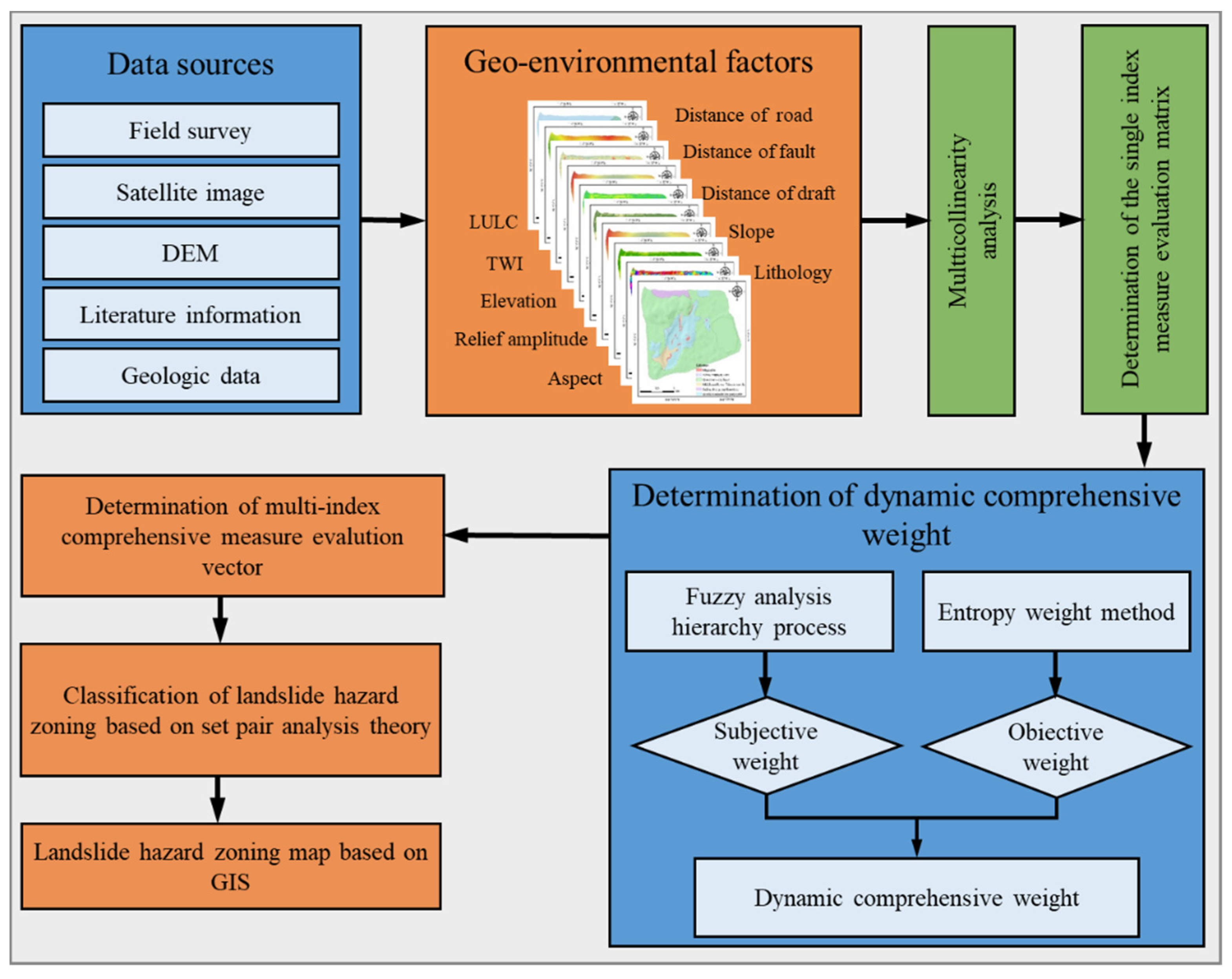
2. Proposed Methodology
2.1. Unascertained Measure Theory
2.2. Set Pair Analysis Theory
2.3. Improved UM-SPA Model
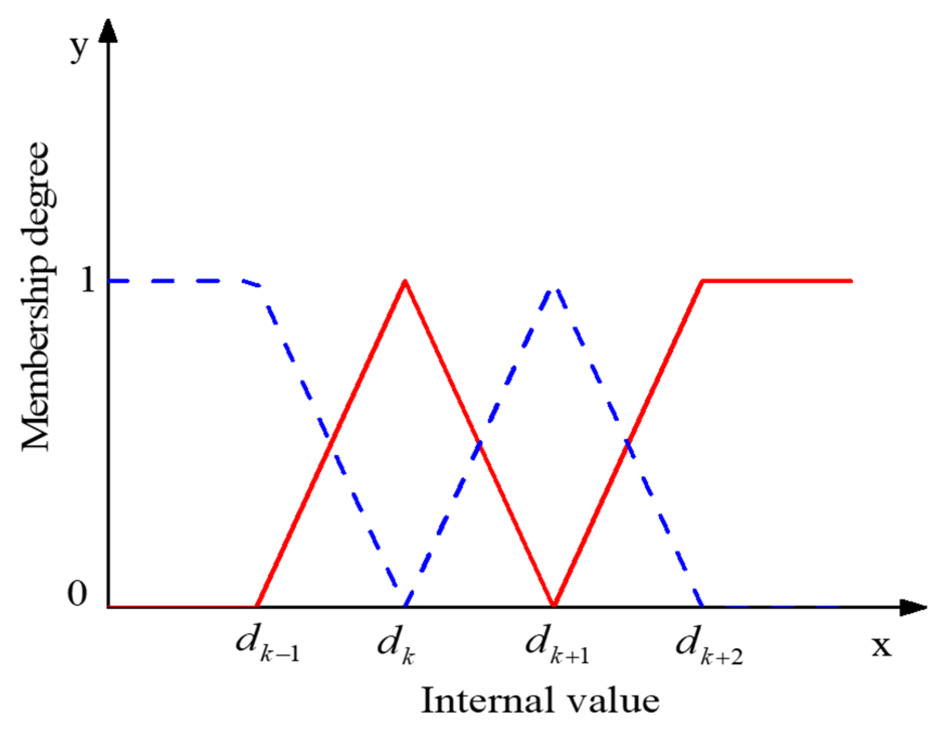
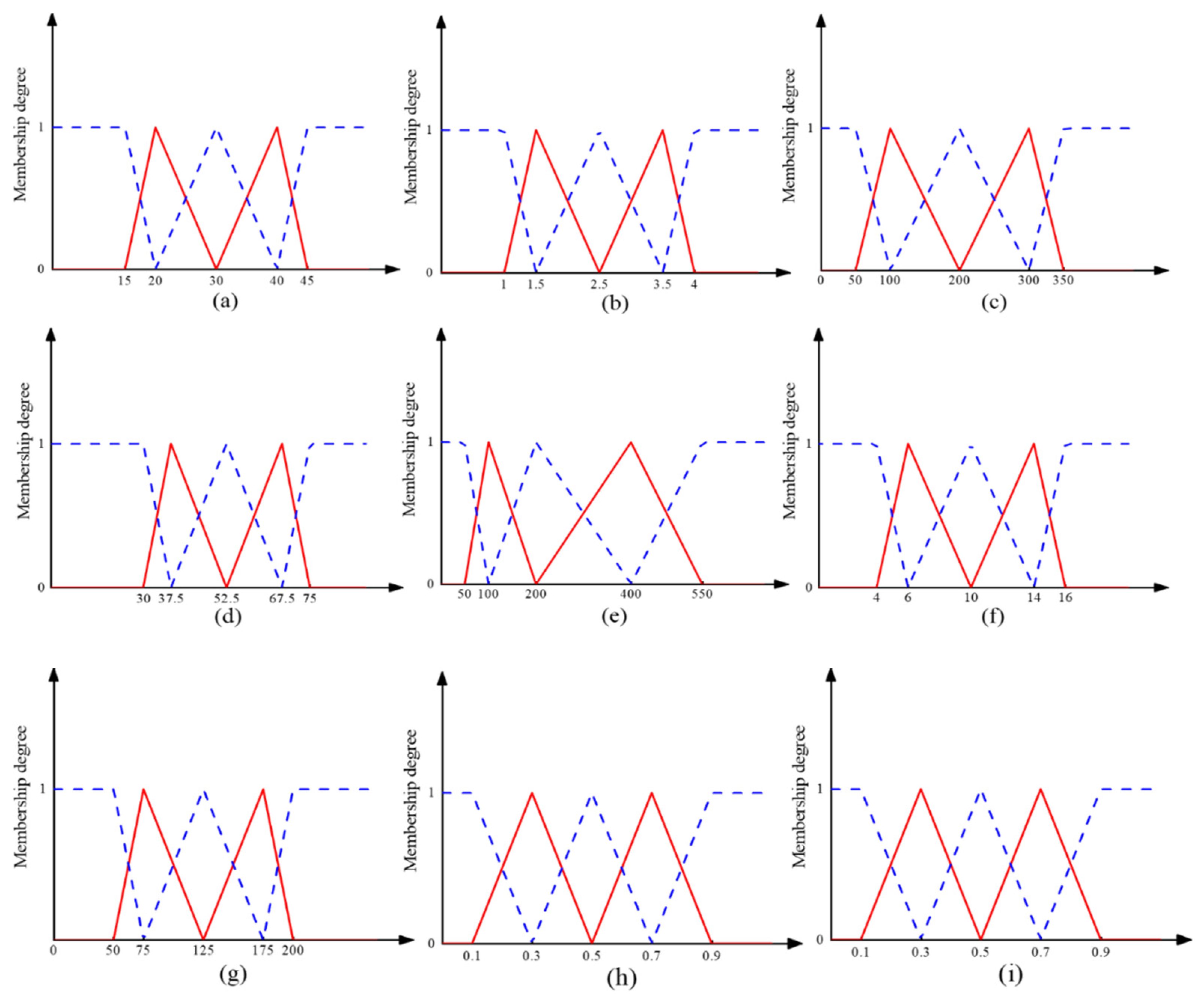
2.3.1. Construct Single Index Unascertained Measure Function
2.3.2. Determine the Subjective Weight Using Fuzzy AHP
2.3.3. Determine the Objective Weight Using Entropy
2.3.4. Calculation of Dynamic Comprehensive Weights
2.3.5. Multi-Index Comprehensive Measure Evaluation Vector
2.3.6. Classification of Landslide Susceptibility Zonation
3. Study Area and Materials
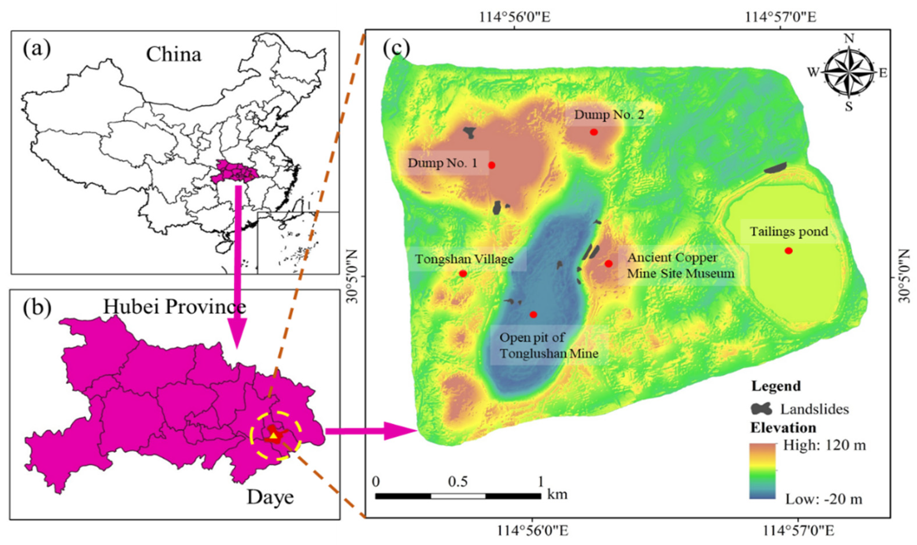
3.1. Study Area
3.2. Landslide Inventory Map
3.3. Landslide Conditioning Factors (LCFs)
4. Landslide Susceptibility Zonation Mapping
4.1. Establishment of Comprehensive Evaluation Index System
4.1.1. Multicollinearity Analysis
4.1.2. Factor Status Grading
4.2. Determination of the Single-Index Measure Evaluation Matrix
4.3. Determination of Dynamic Comprehensive Weights
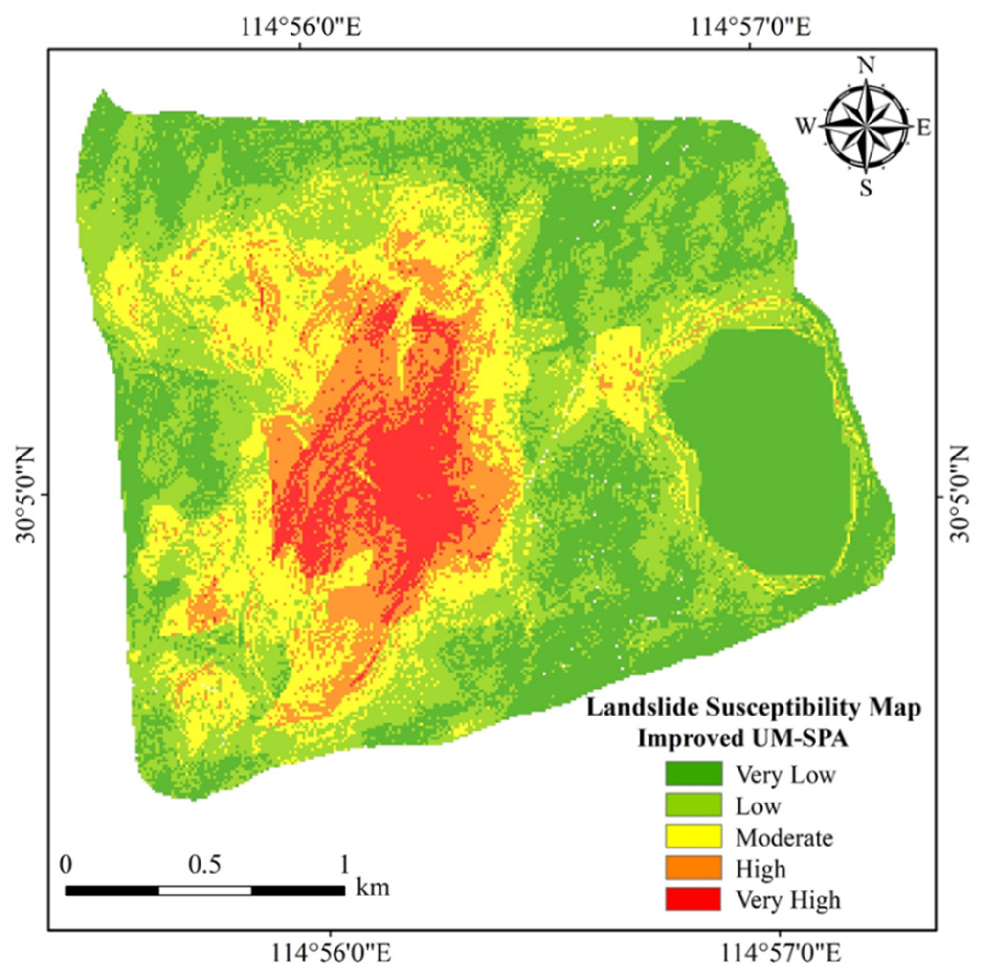
4.4. Landslide Susceptibility Zoning Based on Improved UM-SPA Model
5. Results and Discussion
5.1. Results Analysis
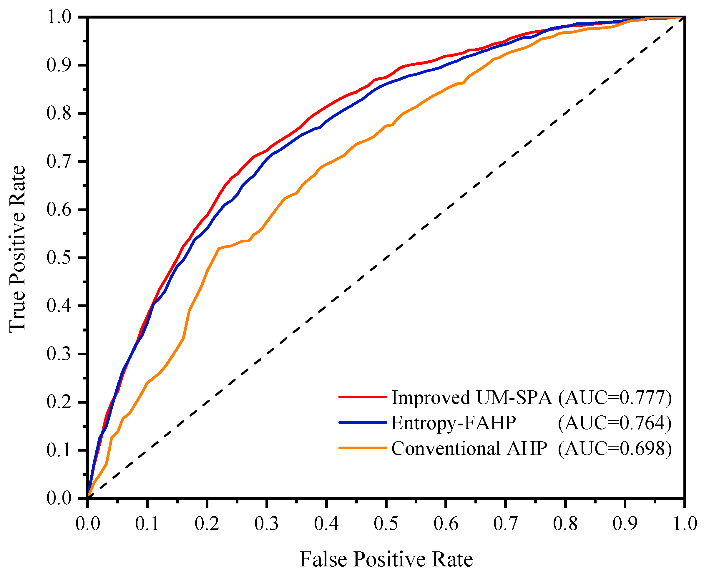
5.2. Model Validation
5.3. Discussion
6. Conclusions
Author Contributions
Funding
Institutional Review Board Statement
Informed Consent Statement
Data Availability Statement
Acknowledgments
Conflicts of Interest
References
- Feizizadeh, B.; Roodposhti, M.S.; Jankowski, P.; Blaschke, T. A GIS-based extended fuzzy multi-criteria evaluation for landslide susceptibility mapping. Comput. Geosci. 2014, 73, 208–221. [Google Scholar] [CrossRef] [PubMed]
- Froude, M.J.; Petley, D.N. Global fatal landslide occurrence from 2004 to 2016. Nat. Hazards Earth Syst. Sci. 2018, 18, 2161–2181. [Google Scholar] [CrossRef]
- Boubazine, L.; Boumazbeur, A.; Hadji, R.; Fares, K. Slope failure characterization: A joint multi-geophysical and geotechnical analysis, case study of Babor Mountains range, NE Algeria. Min. Miner. Depos. 2022, 16, 65–70. [Google Scholar] [CrossRef]
- Yin, K.; Zhu, L. Landslide hazard zonation and application of GIS. Earth Sci. Front. 2001, 8, 279–284. [Google Scholar]
- Dai, F.; Lee, C.; Ngai, Y.Y. Landslide risk assessment and management: An overview. Eng. Geol. 2002, 64, 65–87. [Google Scholar] [CrossRef]
- García-Rodríguez, M.J.; Malpica, J.; Benito, B.; Díaz, M. Susceptibility assessment of earthquake-triggered landslides in El Salvador using logistic regression. Geomorphology 2008, 95, 172–191. [Google Scholar] [CrossRef]
- Bazaluk, O.; Rysbekov, K.; Nurpeisova, M.; Lozynskyi, V.; Kyrgizbayeva, G.; Turumbetov, T. Integrated monitoring for the rock mass state during large-scale subsoil development. Front. Environ. Sci. 2022, 10, 329. [Google Scholar] [CrossRef]
- Guzzetti, F.; Carrara, A.; Cardinali, M.; Reichenbach, P. Landslide hazard evaluation: A review of current techniques and their application in a multi-scale study, Central Italy. Geomorphology 1999, 31, 181–216. [Google Scholar] [CrossRef]
- Achour, Y.; Boumezbeur, A.; Hadji, R.; Chouabbi, A.; Cavaleiro, V.; Bendaoud, E.A. Landslide susceptibility mapping using analytic hierarchy process and information value methods along a highway road section in Constantine, Algeria. Arab. J. Geosci. 2017, 10, 1–16. [Google Scholar] [CrossRef]
- Chen, G.; Li, T.; Zhang, G.; Yin, H.; Zhang, H. Temperature effect of rock burst for hard rock in deep-buried tunnel. Nat. Hazards 2014, 72, 915–926. [Google Scholar] [CrossRef]
- Pachauri, A.; Pant, M. Landslide hazard mapping based on geological attributes. Eng. Geol. 1992, 32, 81–100. [Google Scholar] [CrossRef]
- Zhao, Y.; Wang, R.; Jiang, Y.; Liu, H.; Wei, Z. GIS-based logistic regression for rainfall-induced landslide susceptibility mapping under different grid sizes in Yueqing, Southeastern China. Eng. Geol. 2019, 259, 105147. [Google Scholar] [CrossRef]
- Chen, G.; Li, H.; Wei, T.; Zhu, J. Searching for multistage sliding surfaces based on the discontinuous dynamic strength reduction method. Eng. Geol. 2021, 286, 106086. [Google Scholar] [CrossRef]
- Zhou, S.; Zhou, S.; Tan, X. Nationwide susceptibility mapping of landslides in Kenya using the fuzzy analytic hierarchy process model. Land 2020, 9, 535. [Google Scholar] [CrossRef]
- Kanungo, D.P.; Arora, M.; Sarkar, S.; Gupta, R. A comparative study of conventional, ANN black box, fuzzy and combined neural and fuzzy weighting procedures for landslide susceptibility zonation in Darjeeling Himalayas. Eng. Geol. 2006, 85, 347–366. [Google Scholar] [CrossRef]
- Saadatkhah, N.; Kassim, A.; Lee, L.M. Qualitative and quantitative landslide susceptibility assessments in Hulu Kelang area, Malaysia. EJGE 2014, 19, 545–563. [Google Scholar]
- Aditian, A.; Kubota, T.; Shinohara, Y. Comparison of GIS-based landslide susceptibility models using frequency ratio, logistic regression, and artificial neural network in a tertiary region of Ambon, Indonesia. Geomorphology 2018, 318, 101–111. [Google Scholar] [CrossRef]
- Senouci, R.; Taibi, N.-E.; Teodoro, A.C.; Duarte, L.; Mansour, H.; Yahia Meddah, R. GIS-based expert knowledge for landslide susceptibility mapping (LSM): Case of mostaganem coast district, west of Algeria. Sustainability 2021, 13, 630. [Google Scholar] [CrossRef]
- Mallick, J.; Singh, R.K.; AlAwadh, M.A.; Islam, S.; Khan, R.A.; Qureshi, M.N. GIS-based landslide susceptibility evaluation using fuzzy-AHP multi-criteria decision-making techniques in the Abha Watershed, Saudi Arabia. Environ. Earth Sci. 2018, 77, 1–25. [Google Scholar] [CrossRef]
- Li, W.; Fang, Z.; Wang, Y. Stacking ensemble of deep learning methods for landslide susceptibility mapping in the Three Gorges Reservoir area, China. Stoch. Environ. Res. Risk Assess. 2021, 36, 2207–2228. [Google Scholar] [CrossRef]
- Park, S.; Choi, C.; Kim, B.; Kim, J. Landslide susceptibility mapping using frequency ratio, analytic hierarchy process, logistic regression, and artificial neural network methods at the Inje area, Korea. Environ. Earth Sci. 2013, 68, 1443–1464. [Google Scholar] [CrossRef]
- Zêzere, J.; Pereira, S.; Melo, R.; Oliveira, S.; Garcia, R.A. Mapping landslide susceptibility using data-driven methods. Sci. Total Environ. 2017, 589, 250–267. [Google Scholar] [CrossRef] [PubMed]
- Ghorbanzadeh, O.; Blaschke, T.; Gholamnia, K.; Meena, S.R.; Tiede, D.; Aryal, J. Evaluation of different machine learning methods and deep-learning convolutional neural networks for landslide detection. Remote Sens. 2019, 11, 196. [Google Scholar] [CrossRef]
- Meng, Q.; Miao, F.; Zhen, J.; Wang, X.; Wang, A.; Peng, Y.; Fan, Q. GIS-based landslide susceptibility mapping with logistic regression, analytical hierarchy process, and combined fuzzy and support vector machine methods: A case study from Wolong Giant Panda Natural Reserve, China. Bull. Eng. Geol. Environ. 2016, 75, 923–944. [Google Scholar] [CrossRef]
- Chen, W.; Sun, Z.; Han, J. Landslide susceptibility modeling using integrated ensemble weights of evidence with logistic regression and random forest models. Appl. Sci. 2019, 9, 171. [Google Scholar] [CrossRef]
- Chen, W.; Pourghasemi, H.R.; Panahi, M.; Kornejady, A.; Wang, J.; Xie, X.; Cao, S. Spatial prediction of landslide susceptibility using an adaptive neuro-fuzzy inference system combined with frequency ratio, generalized additive model, and support vector machine techniques. Geomorphology 2017, 297, 69–85. [Google Scholar] [CrossRef]
- Quan, H.-C.; Lee, B.-G. GIS-based landslide susceptibility mapping using analytic hierarchy process and artificial neural network in Jeju (Korea). KSCE J. Civ. Eng. 2012, 16, 1258–1266. [Google Scholar] [CrossRef]
- Moosavi, V.; Niazi, Y. Development of hybrid wavelet packet-statistical models (WP-SM) for landslide susceptibility mapping. Landslides 2016, 13, 97–114. [Google Scholar] [CrossRef]
- Zhao, H.L.; Yao, L.H.; Mei, G.; Liu, T.Y.; Ning, Y.S. A fuzzy comprehensive evaluation method based on AHP and entropy for a landslide susceptibility map. Entropy 2017, 19, 396. [Google Scholar] [CrossRef]
- Li, J.; Wang, C.; Wang, G. Landslide risk assessment based on combination weighting-unascertained measure theory. Rock Soil Mech. 2013, 34, 468–474. [Google Scholar]
- Wang, G. Unascertained information and its mathematical treatment. J. Harbin Univ. Civ. Eng. Archit. 1990, 23, 1–8. [Google Scholar]
- Zhao, K. Set Pair Analysis and Its Preliminary Application; Zhejiang Science Technology Press: Hangzhou, China, 2000; pp. 1–200. [Google Scholar]
- Chen, W.; Zhang, G.; Jiao, Y.; Wang, H. Unascertained measure-set pair analysis model of collapse risk evaluation in mountain tunnels and its engineering application. KSCE J. Civ. Eng. 2021, 25, 451–467. [Google Scholar] [CrossRef]
- Wu, Q.; Zhao, D.; Wang, Y.; Shen, J.; Mu, W.; Liu, H. Method for assessing coal-floor water-inrush risk based on the variable-weight model and unascertained measure theory. Hydrogeol. J. 2017, 25, 2089. [Google Scholar] [CrossRef]
- Yang, X.; Hao, Z.; Ma, G.; Li, G. Research on slope stability evaluation based on improved set pair analysis method: A case of Tonglvshan open-pit mine. Shock Vib. 2021, 2021, 1–16. [Google Scholar] [CrossRef]
- Liu, Y.Y.; Guo, Z.; Li, Y.; Li, Y. Risk assessment model of highway slope based on entropy weight set pair analysis and vehicle laser scanning. Rock Soil Mech. 2018, 39, 131–141+156. [Google Scholar]
- Zhang, X.; Zhou, S.W.; Lin, P.; Tan, Z.Y.; Chen, Z.; Jiang, S. Slope stability evaluation based on entropy coefficient-set pair analysis. Chin. J. Rock Mech. Eng. 2018, 37, 3400–3410. [Google Scholar]
- Hadji, R.; Rais, K.; Gadri, L.; Chouabi, A.; Hamed, Y. Slope failure characteristics and slope movement susceptibility assessment using GIS in a medium scale: A case study from Ouled Driss and Machroha municipalities, Northeast Algeria. Arab. J. Sci. Eng. 2017, 42, 281–300. [Google Scholar] [CrossRef]
- Saaty, T.L. Decision making—The analytic hierarchy and network processes (AHP/ANP). J. Syst. Sci. Syst. Eng. 2004, 13, 1–35. [Google Scholar] [CrossRef]
- Sur, U.; Singh, P.; Meena, S.R. Landslide susceptibility assessment in a lesser Himalayan road corridor (India) applying fuzzy AHP technique and earth-observation data. Geomat. Nat. Hazards Risk 2020, 11, 2176–2209. [Google Scholar] [CrossRef]
- Chang, D.-Y. Applications of the extent analysis method on fuzzy AHP. Eur. J. Oper. Res. 1996, 95, 649–655. [Google Scholar] [CrossRef]
- Shannon, C.E. A mathematical theory of communication. ACM SIGMOBILE Mob. Comput. Commun. Rev. 2001, 5, 3–55. [Google Scholar] [CrossRef]
- Zhai, Q.; Gu, W.; Zhao, Y. Risk assessment of gas disaster in tunnel construction based on unascertained measurement theory. J. Railw. Sci. Eng. 2021, 18, 803–812. [Google Scholar]
- Huang, D.; Shi, X.; Qiu, X.; Gou, Y. Stability gradation of rock slopes based on multilevel uncertainty measure-set pair analysis theory. J. Cent. South Univ. (Sci. Technol.) 2017, 48, 1057–1064. [Google Scholar]
- Tao, Z.; Zhu, C.; Zheng, X.; He, M. Slope stability evaluation and monitoring of Tonglushan ancient copper mine relics. Adv. Mech. Eng. 2018, 10, 1–16. [Google Scholar] [CrossRef]
- Thai Pham, B.; Shirzadi, A.; Shahabi, H.; Omidvar, E.; Singh, S.K.; Sahana, M.; Talebpour Asl, D.; Bin Ahmad, B.; Kim Quoc, N.; Lee, S. Landslide susceptibility assessment by novel hybrid machine learning algorithms. Sustainability 2019, 11, 4386. [Google Scholar] [CrossRef]
- Wang, W.; Yuan, W.; Zou, L.; Chen, H.; Cheng, R.; Xu, W. Comprehensive regional-scale early warning of water-induced landslides in reservoir areas based on landslide susceptibility assessment. Chin. J. Rock Mech. Eng. 2022, 41, 479–491. [Google Scholar]
- Luo, L.; Pei, X.; Cui, S.; Huang, R.; Zhu, L.; He, Z. Chinese Journal of Rock Mechanics and Combined selection of susceptibility assessment factors for Jiuzhaigou earthquake-induced landslidesEngineering. Chin. J. Rock Mech. Eng. 2021, 40, 2306–2319. [Google Scholar]
- Hussain, M.A.; Chen, Z.; Zheng, Y.; Shoaib, M.; Shah, S.U.; Ali, N.; Afzal, Z. Landslide susceptibility mapping using machine learning algorithm validated by persistent scatterer In-SAR technique. Sensors 2022, 22, 3119. [Google Scholar] [CrossRef] [PubMed]
- Yang, X.; Hou, D.; Hao, Z.; Wang, E. Fuzzy comprehensive evaluation of landslide caused by underground mining subsidence and its monitoring. Int. J. Environ. Pollut. 2016, 59, 284–302. [Google Scholar] [CrossRef]
- Guo, Z.; Yin, K.; Huang, F.; Fu, S.; Zhang, W. Evaluation of landslide susceptibility based on landslide classification and weighted frequency ratio model. Chin. J. Rock Mech. Eng. 2019, 38, 287–300. [Google Scholar]
- Park, I.; Choi, J.; Lee, M.J.; Lee, S. Application of an adaptive neuro-fuzzy inference system to ground subsidence hazard mapping. Comput. Geosci. 2012, 48, 228–238. [Google Scholar] [CrossRef]
- Oh, H.-J.; Lee, S. Assessment of ground subsidence using GIS and the weights-of-evidence model. Eng. Geol. 2010, 115, 36–48. [Google Scholar] [CrossRef]
- Li, Y. Research on the Planning and Design of Tonglv Mountain Mining Park in Daye, Hubei Province; Huazhong Agricultural University: Wuhan, China, 2014. [Google Scholar]
- Das, S.; Sarkar, S.; Kanungo, D.P. GIS-based landslide susceptibility zonation mapping using the analytic hierarchy process (AHP) method in parts of Kalimpong Region of Darjeeling Himalaya. Environ. Monit. Assess. 2022, 194, 234. [Google Scholar] [CrossRef]
- Ghosh, S.; Carranza, E.J.M.; van Westen, C.J.; Jetten, V.G.; Bhattacharya, D.N. Selecting and weighting spatial predictors for empirical modeling of landslide susceptibility in the Darjeeling Himalayas (India). Geomorphology 2011, 131, 35–56. [Google Scholar] [CrossRef]
- Yin, C.; Wang, X.; Zhang, J.; Tian, W. Hazard regionalization of debris flow disasters along highways based on genetic algorithm and cloud model. Chin. J. Rock Mech. Eng. 2016, 35, 2266–2275. [Google Scholar]
- Zhang, J.; Yin, K.; Wang, J.; Liu, L.; Huang, F. Evaluation of landslide susceptibility for Wanzhou district of Three Gorges Reservoir. Chin. J. Rock Mech. Eng. 2016, 35, 284–296. [Google Scholar]
- Wang, J.; Yin, K.; Xiao, L. Landslide susceptibility assessment based on GIS and weighted Information Value: A case study of Wanzhou district, Three Gorges Reservoir. Chin. J. Rock Mech. Eng. 2014, 33, 797–808. [Google Scholar]
- Huang, F.; Yin, K.; Jiang, Y.; Huang, J.; Cao, Z. Landslide susceptibility assessment based on clustering analysis and support vector machine. Chin. J. Rock Mech. Eng. 2018, 37, 156–167. [Google Scholar]


| Linguistic Variables | Triangular Fuzzy Numbers | Reciprocal of Triangular Fuzzy Numbers |
|---|---|---|
| Equally Important | (1,1,1) | (1,1,1) |
| Slightly Important | (2,3,4) | (1/4,1/3,1/2) |
| Moderately Important | (4,5,6) | (1/6,1/5,1/4) |
| Very Important | (6,7,8) | (1/8,1/7,1/6) |
| Extremely Important | (9,9,9) | (1/9,1/9,1/9) |
| Intermediate Value | (1,2,3), (3,4,5), (5,6,7), (7,8,9) | (1/3,1/2,1), (1/5,1/4,1/3), (1/7,1/6,1/5), (1/9,1/8,1/7) |
| S. No. | Conditioning Factor | Data Source | Resolution/Scale | Characteristic Description |
|---|---|---|---|---|
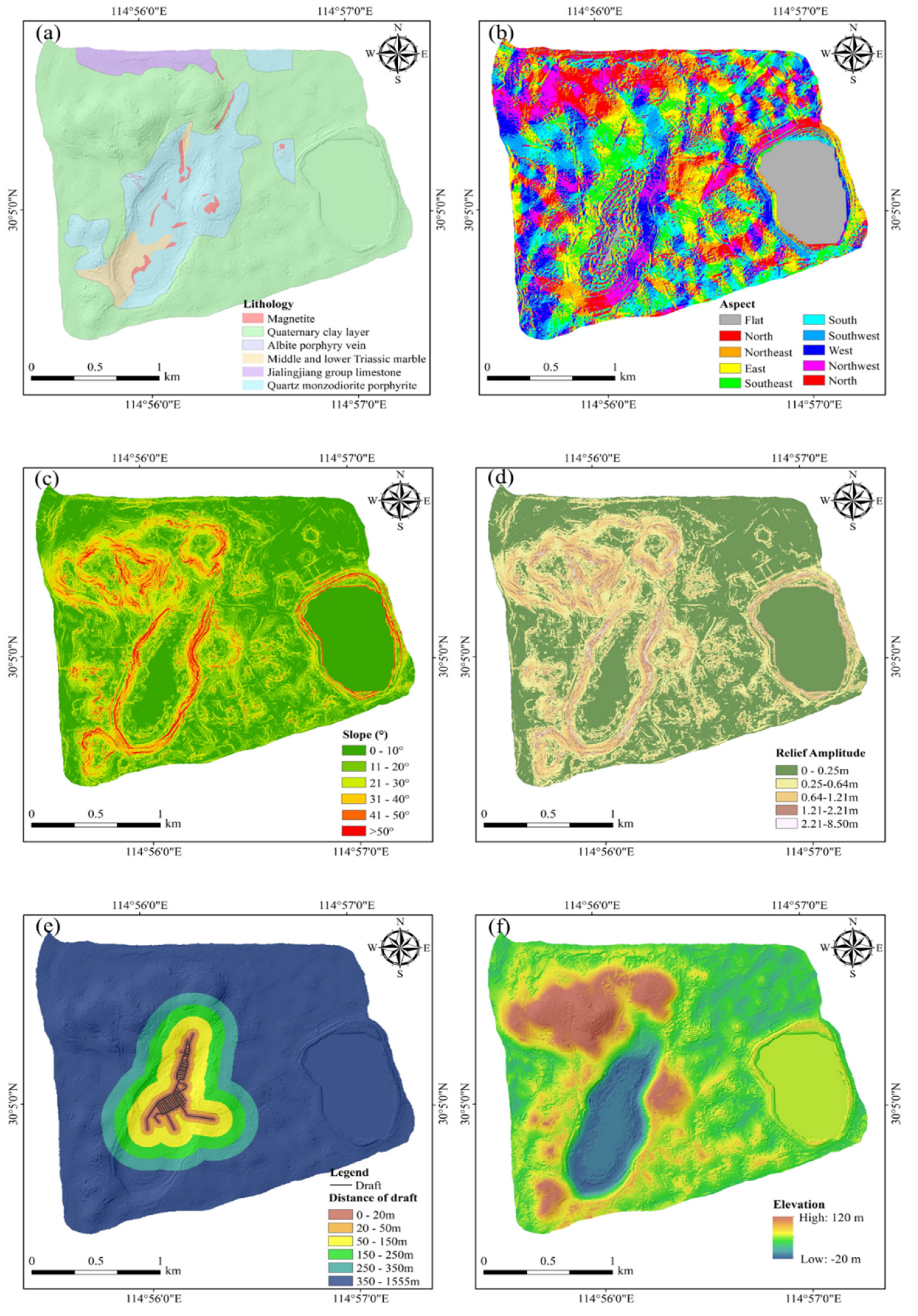
| 1 | Lithology | Geological Map | 1:5000 | Stratum lithology is an important material basis for the formation and development of landslides, which directly affects the physical and mechanical properties of slopes and plays a decisive role in the stability of slopes [46] (Figure 4a). |
| 2 | Aspect | ALOS-PALSAR DEM | 12.5 m | Different slope directions have different solar radiation intensities, resulting in different evaporation of surface water, weathering of rocks and vegetation coverage, which indirectly affect the physical and mechanical properties of rock and soil [48] (Figure 4b). |
| 3 | Slope | ALOS-PALSAR DEM | 12.5 m | The slope provides an empty surface for the formation of the landslide, which has different effects on surface runoff, groundwater recharge/discharge and stress distribution characteristics of the landslide. The bigger the slope, the easier the landslide [40] (Figure 4c). |
| 4 | Relief Amplitude | ALOS-PALSAR DEM | 12.5 m | Relief amplitude is the difference between the highest and lowest elevation in a particular topographic unit, which can reflect the features of topographic relief and is a quantitative index to describe the types of geomorphology [51] (Figure 4d). |
| 5 | Distance of draft | Geological Map | 1:5000 | The historical landslide events in the study area are mainly distributed on the high and steep slope of the east side of the north open pit of Tonglvshan Mine. In order to evaluate the impact of underground mining on the high and steep slope, this paper uses the literature [52,53] method to calculate the tunnel buffer zone using the European distance (Figure 4f). |
| 6 | Elevation | ALOS-PALSAR DEM | 12.5 m | Elevation not only reflects the topographic conditions that directly control the weathering rate and vegetation coverage, but also affects the rainfall intensity that controls the occurrence of landslides [29] (Figure 4g). |
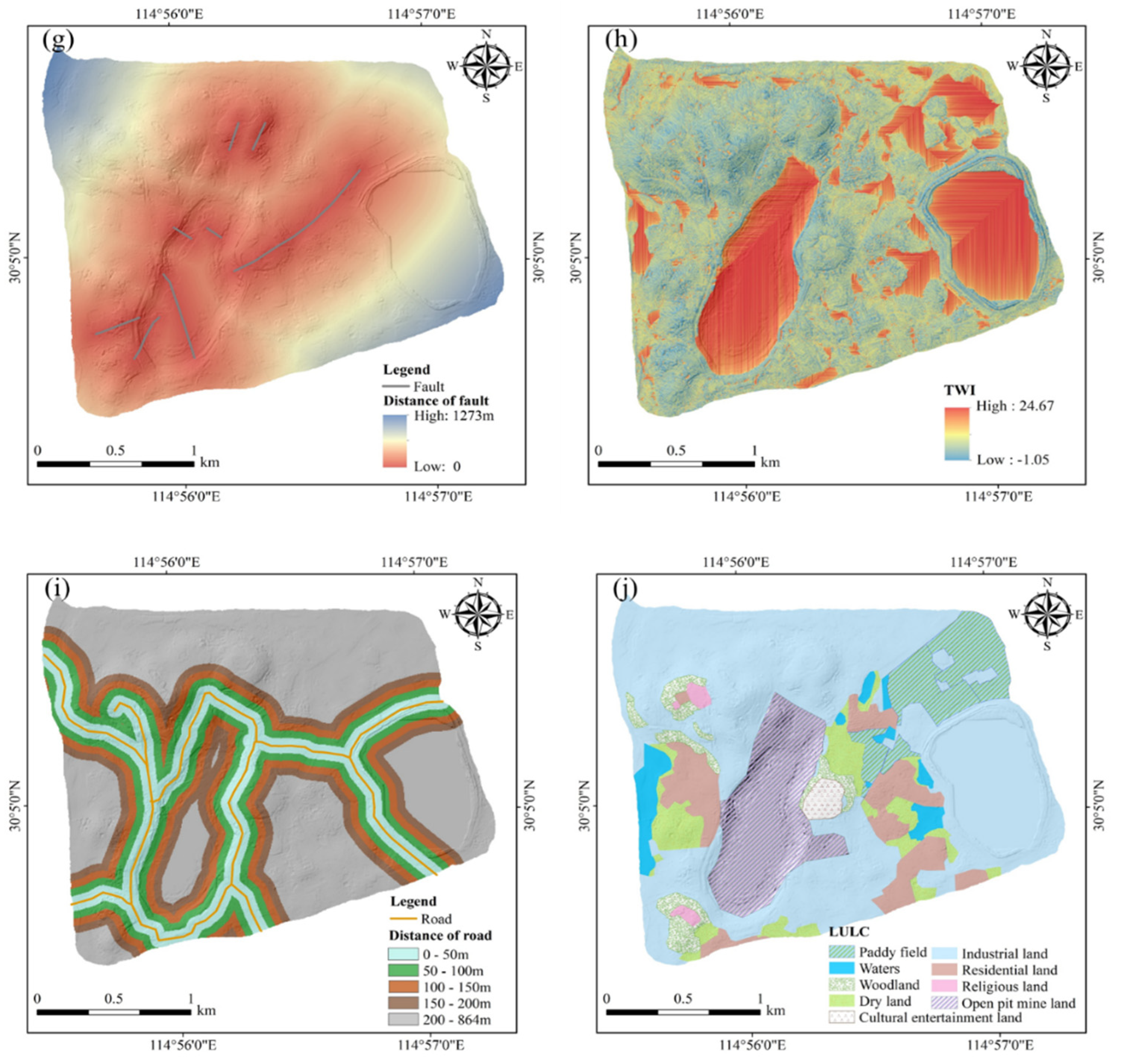
| 7 | Distance of fault | Geological Map | 1:5000 | Geological structure controls the development of joints and fissures in the slope, resulting in the slope being cut into pieces, affecting the development of weak structural planes in the rock mass [17] (Figure 4h). |
| 8 | TWI | ALOS-PALSAR DEM | 12.5 m | TWI comprehensively reflects the impact of terrain and soil characteristics on the water distribution of slope. The higher TWI value may be related to the higher probability of landslide [17] (Figure 4i). |
| 9 | Distance of road | Google Earth Image | 30 m | The road distribution data is vectorized by Google Earth Image, and the European distance is used to calculate the buffer zone of the road [22]. (Figure 4i) |
| 10 | LULC | Literature [54] | - | Obtain and vectorize the current land use map of the site protection area from the literature [14,54]. (Figure 4j). |
| Factors | ||||||||||
|---|---|---|---|---|---|---|---|---|---|---|
| 1 | ||||||||||
| 0.071 | 1 | |||||||||
| 0.129 | 0.180 | 1 | ||||||||
| 0.128 | 0.164 | 0.693 | 1 | |||||||
| −0.423 | −0.073 | −0.280 | −0.267 | 1 | ||||||
| −0.166 | −0.011 | 0.400 | 0.382 | −0.062 | 1 | |||||
| −0.330 | −0.035 | −0.215 | −0.209 | 0.654 | 0.017 | 1 | ||||
| 0.056 | −0.056 | 0.023 | 0.024 | −0.119 | 0.063 | −0.055 | 1 | |||
| −0.102 | −0.037 | −0.312 | −0.308 | 0.349 | −0.178 | 0.334 | −0.055 | 1 | ||
| 0.398 | 0.034 | 0.097 | 0.105 | −0.326 | −0.357 | −0.232 | 0.132 | −0.099 | 1 |
| Primary Evaluation Index | Secondary Evaluation Index | Evaluation Criteria | ||||
|---|---|---|---|---|---|---|
| Very Low (Level I) | Low (Level II) | Moderate (Level III) | High (Level IV) | Very High (Level V) | ||
| terrain | Elevation/m | 0–30 | 30–45 | 45–60 | 60–75 | >75 |
| Slope/(°) | 0–15 | 15–25 | 25–35 | 35–45 | >45 | |
| Aspect | 0.1 | 0.3 | 0.5 | 0.7 | 0.9 | |
| Relief amplitude | 0–1 | 1–2 | 2–3 | 3–4 | >4 | |
| Engineering geological characteristics | Lithology | 0.1 | 0.3 | 0.5 | 0.7 | 0.9 |
| Distance of fault | >550 | 250–550 | 150–250 | 50–150 | 0–50 | |
| Hydrological environment indicators | TWI | 0–4 | 4–8 | 8–12 | 12–16 | >16 |
| Human engineering activity | Distance of draft | >350 | 250–350 | 150–250 | 50–150 | 0–50 |
| Distance of road | >200 | 150–200 | 100–150 | 50–100 | 0–50 | |
| LULC | 0.1 | 0.3 | 0.5 | 0.7 | 0.9 | |
| S. NO. | Evaluation Index Value | |||||||||
|---|---|---|---|---|---|---|---|---|---|---|
| 1 | 0.300 | 0.418 | 1.889 | 0.092 | 1017.085 | 20.472 | 459.061 | 10.214 | 404.607 | 0.300 |
| 2 | 0.300 | 0.686 | 4.184 | 0.188 | 1010.142 | 21.162 | 451.926 | 3.990 | 393.039 | 0.300 |
| 3 | 0.300 | 0.608 | 5.482 | 0.253 | 1002.215 | 22.769 | 444.167 | 6.627 | 380.138 | 0.300 |
| 4 | 0.300 | 0.593 | 6.531 | 0.299 | 992.839 | 24.550 | 435.396 | 4.509 | 366.239 | 0.300 |
| ⋮ | ⋮ | ⋮ | ⋮ | ⋮ | ⋮ | ⋮ | ⋮ | ⋮ | ⋮ | ⋮ |
| 56048 | 0.300 | 0.244 | 1.702 | 0.082 | 1349.518 | 17.899 | 1204.751 | 7.007 | 385.811 | 0.300 |
| 56049 | 0.300 | 0.344 | 3.324 | 0.157 | 1404.219 | 18.720 | 1260.274 | 6.884 | 398.824 | 0.300 |
| 56050 | 0.300 | 0.504 | 4.034 | 0.179 | 1392.165 | 18.495 | 1245.841 | 6.018 | 402.689 | 0.300 |
| 56051 | 0.300 | 0.286 | 1.844 | 0.087 | 1379.279 | 18.388 | 1232.126 | 2.785 | 401.474 | 0.300 |
| Factors | Lithology | Aspect | Slope | Relief Amplitude | Distance of Draft | Elevation | Distance of Fault | TWI | Distance of Road | LULC |
|---|---|---|---|---|---|---|---|---|---|---|
| Lithology | (1,1,1) | (1,2,3) | (1,2,3) | (3,4,5) | (1,2,3) | (1,2,3) | (3,4,5) | (3,4,5) | (2,3,4) | (2,3,4) |
| Aspect | (1/3,1/2,1) | (1,1,1) | (1/2,1,1) | (2,3,4) | (1/2,1,1) | (1,1,2) | (2,3,4) | (2,3,4) | (1,2,3) | (1,2,3) |
| Slope | (1/3,1/2,1) | (1,1,2) | (1,1,1) | (2,3,4) | (1,1,2) | (1/2,1,1) | (2,3,4) | (2,3,4) | (1,2,3) | (1,2,3) |
| Relief amplitude | (1/5,1/4,1/3) | (1/4,1/3,1/2) | (1/4,1/3,1/2) | (1,1,1) | (1/4,1/3,1/2) | (1/4,1/3,1/2) | (1/2,1,1) | (1,2,3) | (1/3,1/2,1) | (1/3,1/2,1) |
| Distance of draft | (1/3,1/2,1) | (1,1,2) | (1/2,1,1) | (2,3,4) | (1,1,1) | (1,1,2) | (2,3,4) | (2,3,4) | (1,2,3) | (1,2,3) |
| Elevation | (1/3,1/2,1) | (1/2,1,1) | (1,1,2) | (2,3,4) | (1/2,1,1) | (1,1,1) | (2,3,4) | (2,3,4) | (1,2,3) | (1,2,3) |
| Distance of fault | (1/5,1/4,1/3) | (1/4,1/3,1/2) | (1/4,1/3,1/2) | (1,1,2) | (1/4,1/3,1/2) | (1/4,1/3,1/2) | (1,1,1) | (1/2,1,1) | (1/3,1/2,1) | (1/3,1/2,1) |
| TWI | (1/5,1/4,1/3) | (1/4,1/3,1/2) | (1/4,1/3,1/2) | (1/2,1/2,1) | (1/4,1/3,1/2) | (1/4,1/3,1/2) | (1,1,2) | (1,1,1) | (1/3,1/2,1) | (1/3,1/2,1) |
| Distance of road | (1/4,1/3,1/2) | (1/3,1/2,1) | (1/3,1/2,1) | (1,2,3) | (1/3,1/2,1) | (1/3,1/2,1) | (1,2,3) | (1,2,3) | (1,1,1) | (1/2,1,1) |
| LULC | (1/4,1/3,1/2) | (1/3,1/2,1) | (1/3,1/2,1) | (1,2,3) | (1/3,1/2,1) | (1/3,1/2,1) | (1,2,3) | (1,2,3) | (1,1,2) | (1,1,1) |
| Factors | |||||||||||
|---|---|---|---|---|---|---|---|---|---|---|---|
| - | 0.710 | 0.723 | 0.061 | 0.723 | 0.710 | 0.000 | 0.000 | 0.388 | 0.419 | ||
| 1.000 | - | 0.000 | 0.355 | 0.000 | 0.000 | 0.275 | 0.267 | 0.680 | 0.700 | ||
| 1.000 | 0.000 | - | 0.342 | 1.000 | 1.000 | 0.259 | 0.251 | 0.675 | 0.696 | ||
| 1.000 | 1.000 | 1.000 | - | 0.000 | 0.000 | 0.904 | 0.863 | 1.000 | 1.000 | ||
| 1.000 | 0.000 | 0.000 | 0.342 | - | 0.000 | 0.259 | 0.251 | 0.675 | 0.696 | ||
| 1.000 | 0.000 | 0.000 | 0.355 | 0.000 | - | 0.275 | 0.266 | 0.680 | 0.700 | ||
| 1.000 | 1.000 | 1.000 | 1.000 | 1.000 | 1.000 | - | 0.949 | 1.000 | 1.000 | ||
| 1.000 | 1.000 | 1.000 | 1.000 | 1.000 | 1.000 | 1.000 | - | 1.000 | 1.000 | ||
| 1.000 | 1.000 | 1.000 | 0.721 | 1.000 | 1.000 | 0.633 | 0.609 | - | 0.000 | ||
| 1.000 | 1.000 | 1.000 | 0.713 | 1.000 | 1.000 | 0.623 | 0.599 | 0.000 | - | ||
| 1.000 | 0.710 | 0.723 | 0.061 | 0.723 | 0.710 | 0.259 | 0.251 | 0.388 | 0.419 | ||
| Factors | ||||||||||
|---|---|---|---|---|---|---|---|---|---|---|
| Weight | 0.191 | 0.135 | 0.138 | 0.012 | 0.138 | 0.135 | 0.049 | 0.048 | 0.074 | 0.080 |
| Susceptibility Level | Ⅰ | Ⅱ | Ⅲ | Ⅳ | Ⅴ |
|---|---|---|---|---|---|
| Grade description | Very low | Low | Moderate | High | Very high |
| Judgment interval | (0.6, 1.0] | (0.2, 0.6] | (−0.2, 0.2] | (−0.6, −0.2] | [−1.0, −0.6] |
| LCF | ||||||||||
|---|---|---|---|---|---|---|---|---|---|---|
| 1 | ||||||||||
| 1/2 | 1 | |||||||||
| 1/2 | 1 | 1 | ||||||||
| 1/3 | 1/3 | 1/5 | 1 | |||||||
| 1/2 | 4 | 1 | 5 | 1 | ||||||
| 1/2 | 1/2 | 1/3 | 4 | 1 | 1 | |||||
| 1/3 | 1/2 | 1/3 | 2 | 1/3 | 1/4 | 1 | ||||
| 1/3 | 1/3 | 1/3 | 1 | 1/5 | 1/4 | 1/2 | 1 | |||
| 1/3 | 1/2 | 1/3 | 3 | 1/5 | 1/5 | 1 | 3 | 1 | ||
| 1/3 | 1/2 | 1/2 | 3 | 1/3 | 1/3 | 2 | 1/2 | 2 | 1 | |
| 0.188 | 0.111 | 0.151 | 0.031 | 0.180 | 0.133 | 0.049 | 0.042 | 0.533 | 0.062 |
Disclaimer/Publisher’s Note: The statements, opinions and data contained in all publications are solely those of the individual author(s) and contributor(s) and not of MDPI and/or the editor(s). MDPI and/or the editor(s) disclaim responsibility for any injury to people or property resulting from any ideas, methods, instructions or products referred to in the content. |
© 2023 by the authors. Licensee MDPI, Basel, Switzerland. This article is an open access article distributed under the terms and conditions of the Creative Commons Attribution (CC BY) license (https://creativecommons.org/licenses/by/4.0/).
Share and Cite
Yang, X.; Hao, Z.; Liu, K.; Tao, Z.; Shi, G. An Improved Unascertained Measure-Set Pair Analysis Model Based on Fuzzy AHP and Entropy for Landslide Susceptibility Zonation Mapping. Sustainability 2023, 15, 6205. https://doi.org/10.3390/su15076205
Yang X, Hao Z, Liu K, Tao Z, Shi G. An Improved Unascertained Measure-Set Pair Analysis Model Based on Fuzzy AHP and Entropy for Landslide Susceptibility Zonation Mapping. Sustainability. 2023; 15(7):6205. https://doi.org/10.3390/su15076205
Chicago/Turabian StyleYang, Xiaojie, Zhenli Hao, Keyuan Liu, Zhigang Tao, and Guangcheng Shi. 2023. "An Improved Unascertained Measure-Set Pair Analysis Model Based on Fuzzy AHP and Entropy for Landslide Susceptibility Zonation Mapping" Sustainability 15, no. 7: 6205. https://doi.org/10.3390/su15076205
APA StyleYang, X., Hao, Z., Liu, K., Tao, Z., & Shi, G. (2023). An Improved Unascertained Measure-Set Pair Analysis Model Based on Fuzzy AHP and Entropy for Landslide Susceptibility Zonation Mapping. Sustainability, 15(7), 6205. https://doi.org/10.3390/su15076205