1. Introduction
A sustainable solution for rural water delivery requires accurate water infrastructure assessment and efficient data processing techniques. These techniques need data, which should come from regular usage of the water infrastructure. However, most rural water installations lack accurate data from the available repository [
1]. Therefore, with inadequate, partial, or missing data regarding the smart water taps, it is difficult to develop a comprehensive failure prediction model or an early warning system. Furthermore, investment in extensive inspection and data-gathering programmes on smart rural taps to overcome data gaps may not be financially feasible for rural water management agencies [
2]. So, to achieve failure prediction for rural water taps, the available time series data generated from the system usage and data manipulation is sufficient for critical analysis irrespective of the discrepancies.
Part of the aim of this paper is to develop a failure prediction model for smart water taps to support proactive maintenance, which can help provide a sustainable water supply to rural communities in sub-Saharan Africa and similar contexts. Solar-powered smart water taps (SWT) deployed to rural areas in some parts of Africa are perceived as low-cost and reliable water supply sources for domestic use in the region. These SWTs, often referred to as e-taps, dispense water when a pre-paid token comes in contact with them. During their functional time, the smart taps generate time series datasets that can be analysed for the purpose of developing a failure prediction model that will ensure a functional sustainability of the water taps. This study also shows the importance of appropriately preparing a case study dataset for time series failure prediction problems. The study also ensures that existing water taps in rural communities in Africa are sustained and managed in a way that satisfies the current water and future socioeconomical ecological demand of sub-Saharan Africa. Furthermore, it shows the procedures for preparing time series datasets for efficient analysis with machine-learning (ML) techniques. Finally, because of the inconsistencies in the case study dataset, the research presents a method for data imputation to correct data discrepancy in the dataset.
Most time series can be defined as a set of generated observations
acquired at specified time steps
. On the other hand, a discrete time series can be described as one in which a discrete set
(where
) of times at which observations were made, for example, recording water usage observations at fixed time intervals [
3].
For most data-driven applications, the ML learning paradigm—a time series data representation and generalisation of the learning structure used on datasets—is mostly adopted. However, the data representation impacts the machine-learning performance based on the quality of the available dataset. Therefore, poor data representation may reduce the machine-learning model’s performance, while better data representation can result in a better-performing ML model [
4]. Therefore, selecting appropriate feature values for feature construction and data representations from an input dataset is a core element of the ML principle. In addition, an efficient feature engineering task requires some time, which takes a larger part of the time required to build an ML model. This task is also domain-specific as it requires human input. Therefore, the dataset should follow the standard time series data collection method [
5].
When handling missing data in a dataset, two helpful sides of a case study can identify the impact on the time series prediction result. Firstly, the quantity of missing data is beneficial for our case study. Therefore, the quantity of missing data directly impacts the prediction result and conclusion. The second practical aspect that impacts the prediction result is the cause of missing data in a case study. Therefore, the most important step in analysing a time series is describing the dataset and selecting appropriate computational or mathematical models for the interest data.
Furthermore, in order to accommodate future observations (new data), this study assumes that each observation
is a subset of a given random variable
. Finally, the proposed research assumes that a time series can be described as a collection of random variables plotted according to the order obtained over time. For example,
(where
denote values recorded at each time step) is a time series with a sequence of random variables at different timestamps [
6].
This research’s main contribution involves preparing data for time series failure prediction, emphasising the need for data cleaning and procedures for missing data imputation. The proposed method of the data preparation has the following features:
- (1)
Data preparation through missing data imputation using the generative adversarial network (GAN);
- (2)
BiGRU saves computational time by combining the model’s cell state and hidden state during data imputation;
- (3)
Analysis of the missing data proportion in the dataset;
- (4)
Identification of the dataset patterns.
2. Classification of Missing Data
Missingness in datasets can be described as missing data values from a sample dataset [
2,
7]. The source of missingness in a dataset is very important in data analysis because it affects the technique required to address the problem [
8]. Several underlying factors can cause missing data in a case study:
lost or forgotten data value;
missing value due to non-applicability to the instances of the case study event;
missing value due to irrelevance to the instances of the study.
For example, SWT data variables can be measured; however, the record of such variable values may be missing for unknown reasons. Additionally, the failure of the SWT sensors (the case study), database communication error, human error, electrical component failure or related factors can cause a dataset to be missing.
On the other hand, the SWT variable may not be recorded over a given period for unknown reasons. For instance, missing records over a long period or at random. Additionally, data may not be captured because it is recorded but not useful to a study. In dealing with missing data from the SWT case study, a distinction is made between missing data due to identifiable reasons and missing data due to unidentifiable reasons. In the former case, data imputation for missing data due to identifiable factors can cause a bias in the result of a study [
9]. Therefore, imputing data for unidentifiable reasons can be done based on the assumption that the data are missing randomly. Thus, while data missing for identifiable reasons are non-recoverable, data can be recovered for unidentifiable reasons.
Data imputation is a challenging task that consumes time. Selecting relevant variables from a dataset involves the identification of useful potential predictor subsets from a large candidate set [
10]. Therefore, the general steps involved in handling missing data include:
Analysis of the missing data proportion in the dataset;
Identification of the dataset patterns;
Detecting the cause of missing data;
Selecting the appropriate data imputation method.
The mathematical definition of missing data is as shown in Equations (1)–(3) [
8] (Salgado, Azevedo, Proen, & Vieira, 2016):
where:
—dataset
—observed data
—missing data
A binary response for each observation is designed to determine the missing observation, as shown in Equation (2):
where:
—binary response
However, a probability
can be used to describe the missing value mechanisms to show that observation may be missing given
and
:
The three missing data mechanisms are subject to the dependence of the response probability (i.e., whether or not the response probability depends on the observed or missing data values).
2.1. Missing Completely at Random (MCAR)
This phenomenon occurs when a dataset’s missing values are dependent on the measurement of the observed and unobserved data values. Given
with some missing values, the missing values are MCAR if the likelihood of
missing data is unrelated to
values or other data variables. For example, if the data value of every sixth event in the e-tap is not recorded or omitted, the mechanism for that missing data is MCAR [
11,
12]. Therefore, the probability of a missing observation depends on itself alone and thus reduces to:
2.2. Missing at Random (MAR)
The MAR mechanism gives a weaker assumption than the previous mechanism (MCAR). The MAR mechanism is a probability of a missing data value relating to the observable data only (i.e., statistically, the observed data are related to the missing data) [
13]. Therefore, estimating the missing data value from the observed data is possible. Furthermore, the probability of
missing data values is not related to the values of
. The mathematical equation for this is shown in Equation (5):
2.3. Missing Not at Random (MNAR)
The MNAR mechanism allows missing data to depend on unobserved data values, a missing mechanism where both MCAR and MAR do not apply. Therefore, determining the missing mechanism may be impossible if the data are unseen. In MNAR, the whole data distribution is only identifiable with further assumptions [
14]. The next section of this paper shows the characteristics of the case study dataset, which aids in identifying the missingness mechanism to adopt in handling the challenge of missing data and data inconsistencies found in the dataset.
3. Materials and Methods
This research implementation was in collaboration with an industry partner. This industry partner was the data provider, including real historical data collected from the SWT setups’ daily usage over one year, from 2 August 2017 to 11 July 2018, from 27 water points at Jarreng village in the Gambia, West Africa. The data represented the water system’s activity, which was collected in real time through the NFC component of the SWT via a remote server. The data also contained 1,054,009 samples with varying discrepancies and tap performances. A missing rate was used to randomly generate missing samples, while the data distribution and imputation were achieved using the GAN and BiGRU methods. The data observation had an interval of 1 h, which was used to accommodate all activities of the SWT.
The computing environment was an HP workstation with 16 GB of RAM and one terabyte of memory. The training environment was the Anaconda distribution of Python 3.0 and TensorFlow version 1.7.1 installed on the workstation. The evaluation metric was the root mean squared error (RMSE).
3.1. Problem Formulation
Data imputation is a challenging task that consumes time. Moreover, selecting relevant variables from a dataset involves the identification of useful potential predictor subsets from a large candidate set [
10]. Therefore, we defined missing data as presented in Equation (1).
Given the SWT setups with taps, the SWT time series recorded at times with samples (where —-dimensional sample; —original space dimensionality; —number of data points).
In this formulation, the missing data pattern and location are deemed important. Therefore, we intend to show how to recover some of the unknown data values from the case study noisy dataset . We also assumed that with values in is a mask matrix where which indicates the existence or non-existence of a dataset value. For example, if exist and 0 otherwise. The aim is to impute missing data values as closely as possible to the existing data value. Therefore, we impute the SWT dataset to fill in the missing values based on their spatiotemporal relation.
In order to present a three-dimensional SWT multivariate example, four SWTs with three observations are shown in the matrix in Equations (6)–(9).
Next, a new matrix is defined thus:
This matrix records the time between the last value and the current value.
3.2. Characteristics of Data in the Investigated SWTs
Following daily use, the SWT generates a large quantity of time series datasets, which contain much information about the system’s behaviour. Therefore, it is important to have a time series dataset with continuous intervals without any breaks between them. For example, it is acceptable to have a dataset that consists of only
Year–Month–Day or other time elements alone, such as
Hour–Minute–Second (or even both). However, the time intervals must be provided in a continuous time step. For example,
Figure 1a shows some data inconsistencies. Although the data structure looks fine, the time element contains inconsistent time steps. For example, 04:22:00 precedes 04:22:09 (a 9 s time step), after which the minutes and seconds change to 3 and 4 s intervals.
Figure 1b is another sample of incoherent time steps found in the
DateTime column of the dataset.
It is scientifically advisable that the time series dataset or sample be collected in a manner (i.e., stochastically) that reflects the daily, monthly or strictly adheres to hour/minute/second intervals [
3]. Another technique is to roll up the time steps and take the statistical mean value of the columns [
15].
Figure 2 also shows examples of missing day and month values. For example, from 2018-07-11, the next date is shown as 2019-12-04. Thus, a few months were missing from the list of months in some of the datasets.
To further emphasise the noise in the dataset due to a poor data collection method,
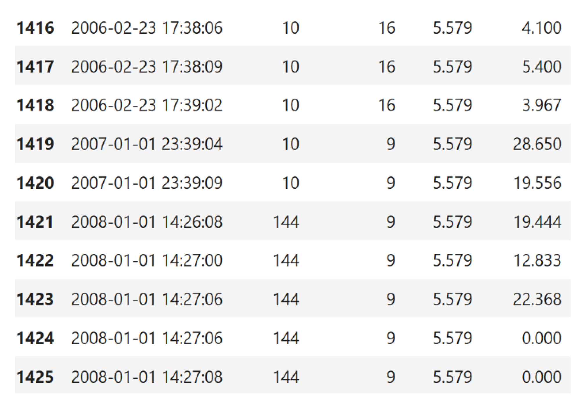
Figure 3 shows an example of missing years, months and days (inclusive of a missing timestamp as well). For example, the year 2006 ends in February, and the next time step begins in January 2007. Similarly, only two time steps exist in the real data of 2007.
3.3. Missingness in a Dataset
In order to effectively handle missingness in a dataset, the method used should be peculiar to the case study datasets, the cause of the missingness and the percentage of missing data in the case study. However, in selecting the model for our study, we considered the simplicity of the missing data handling model and its ability to minimise the bias it introduces to the dataset. We did this to ensure that high-quality datasets could be used for modelling. For example, the water tap dataset contained many missing values in some variables (e.g.,
Figure 2 and
Figure 3). Furthermore, in certain variables (e.g.,
Figure 3), incorrect values were also found.
An initial exploratory data analysis (EDA) was performed on the dataset [
16]. The EDA aids in iteratively interacting with the dataset to extract relevant information from the case study. For example, the information could be the quality, the shape and relevant insights about the dataset.
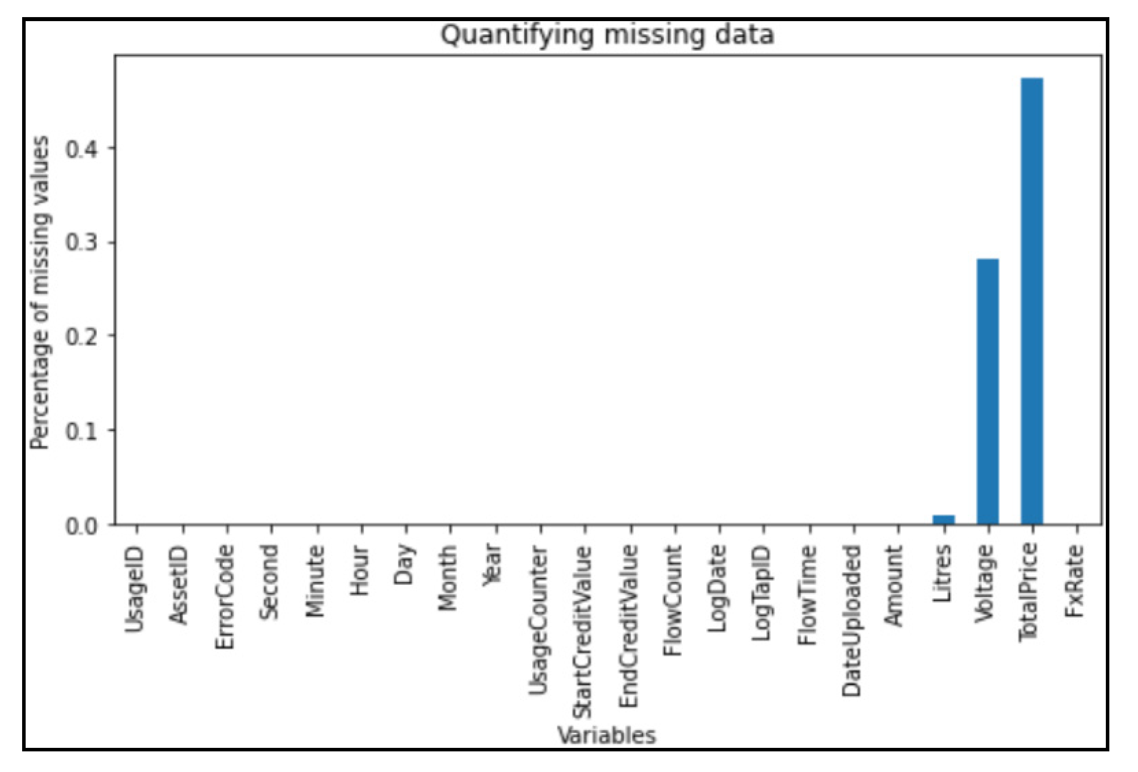
Figure 4 shows an initial EDA performed on the historical dataset acquired from the study location.
Figure 4 depicts the data variable and their corresponding missing values. From the plot, the variables; Litre, Voltage, TotalPrice and the amount spent all have significant missing dataset values, which can affect the result of any data analysis. Finally, after ascertaining the missingness in the case study dataset, we then formulate the missing data as described in
Section 3.4.
3.4. Missing Data Formulation
The missing data pattern and location are deemed important in the missing data formulation. Therefore, we show how to recover some of the unknown data values from the case study noisy dataset . It is assumed that with values in is a mask matrix where indicates the existence or non-existence of a dataset value. For example, if exist and 0 otherwise. The aim is to impute missing data values as closely as possible to the existing data value. Therefore, the imputation of the SWT dataset is to fill in the missing values based on their spatiotemporal relation.
3.5. Implementation of Missing Data Imputation
This section gives a detailed description of the proposed SWT data imputation methods. The data imputation approach used in this work involves using GAN and BiGRU. Each approach plays a significant role in achieving a clean dataset for time series failure prediction in SWTs.
3.5.1. Generative Adversarial Network (GAN)
Goodfellow [
17] proposed the generative adversarial network, which constitutes two parts, namely: the generator network (
) and the discriminator network (
). We applied the generator network component to map random SWT data noise (i.e., the low-dimensional vectors) to the data samples. Secondly, we used the discriminator network to receive low- and high-dimensional data values and distinguish the two sets [
18]. Then, we simultaneously trained the generator and discriminator net to compete during training. Therefore, the GAN method generated a new synthetic dataset in line with the training set distribution.
On the other hand, the discriminator network (𝔇) was used to distinguish between the forged time series and the real SWT dataset because it had access to the real SWT and forged data samples. Finally, we used the value function
to evaluate the model learning cost. The learning process involves the computation shown in Equation (10):
where:
Therefore, the generator parameter stays fixed while the discriminator is updated or vice versa. However, in practice, the traditional GAN suffers instability (mode collapse). We further introduced the training stability by introducing Wasserstein GAN (WGAN), which is formulated as shown in:
Therefore, to efficiently impute missing SWT data values, we used the bidirectional GRU to compress the missing e-tap data value into the low-dimensional vector. Then, the low-dimensional vector was applied to the reconstruction of the forged SWT time series () in order to confuse the discriminator network. The discriminator generator, on the other hand, harnessed the recursive function to create a distinction between and .
3.5.2. Bidirectional Gated Recurrent Unit (BiGRU)
It is noteworthy that the SWT data value contained rough time lags that were handy in the method development. In cases where past observations were missing over a significant period, we applied the BiGRU to introduce a decay vector
, which decreased the GRU memory by combining the cell state and the input gate, as shown in Equation (12).
where:
and —training parameters
Therefore, based on Equation (12), the decay vector
is a value between 0–1, but it is not zero. Following this, the GRU hidden state
is updated through a multiplication (through a listwise manner) of the decay vector
as shown in Equation (13):
where:
—the hidden state
However, because the method uses a BiGRU, we designed the imputation process to correct missing data values and simultaneously save implementation time. Thus, two hidden states are added up, as shown in Equation (14):
Updating the BiGRU for SWT missing data imputation is as follows:
where
—activation function
and —reset gates
and —reset gates
, , and —hidden states
, , , , and —learning parameters
Based on the preceding equations, the decay vector computation ensures that the value of the decay vector decreases as the time lag increases.
3.6. The Proposed GAN for SWT Dataset Imputation
Generally, random noises are passed to the GAN model’s generator network to generate a synthesised set of data values. However, in the proposed method, the SWT dataset already contains highly noisy sets of time series, which makes the addition of new noises appropriate. Usually, the incomplete SWT dataset would need additional noise before the model training begins.
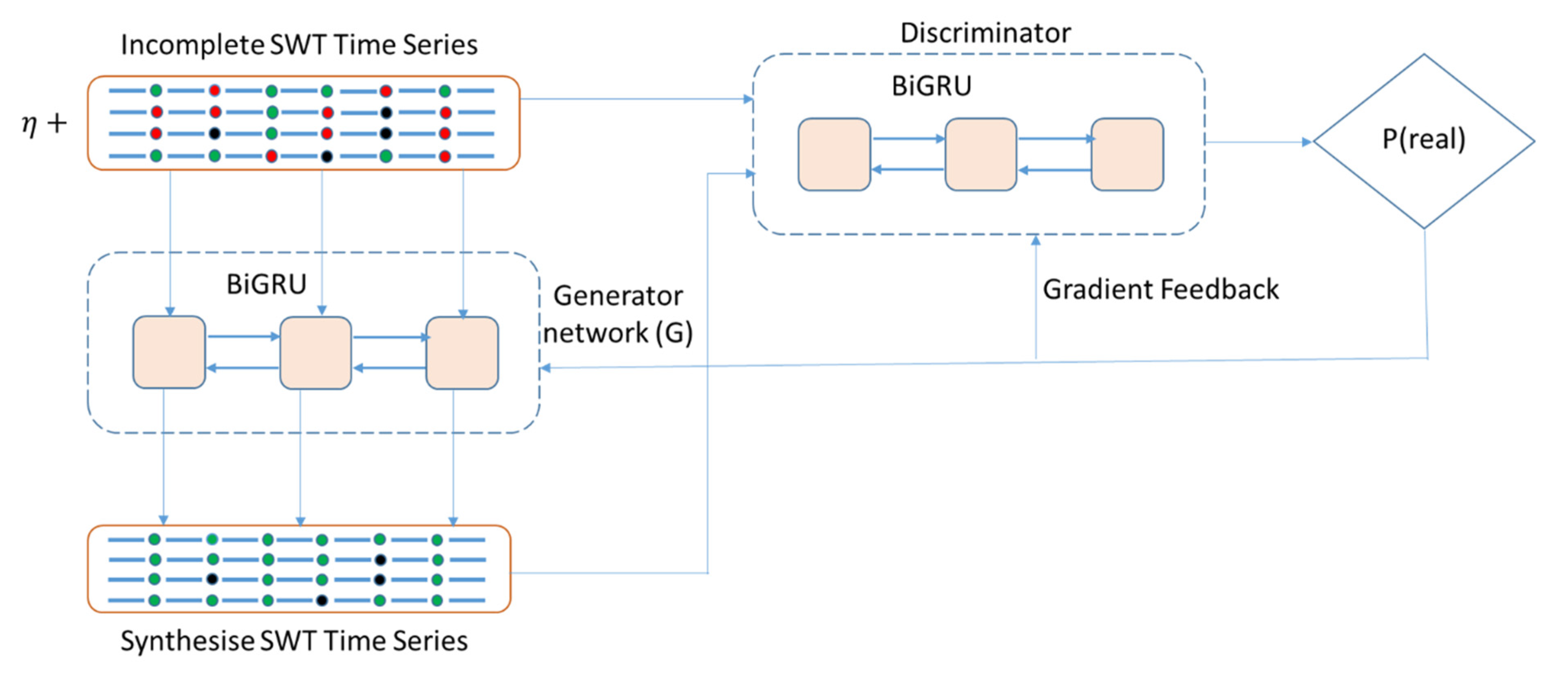
Figure 5 shows the proposed method and how it tries to reconstruct the required synthesised time series
.
From
Figure 5, the incomplete SWT time series is harnessed by the generator network to impute samples from which the synthesised time series
was generated, while the BiGRUI is the component we used to construct the generator and discriminator networks. The discriminator network, on the other hand, compares the synthesise time series
with the actual time series
values and attempts to distinguish between the
and the
values. Convergence of the discriminator network occurs where a distinction between the two variables’ values cannot be achieved. The training of the denoiser model is as shown in Equation (23):
The generator network produces new time series similar to the actual SWT time series , by adding to the generator’s loss function a squared error metric. This process makes it easy to impute the values of the actual SWT time series with the synthesise time series . Therefore, the BiGRUI accepts as input for processing. After the time series processing, the recurrent neural network’s hidden state connects to the fully connected layer of the network. In turn, the fully connected layer of the network then compresses the low-dimensional vector as output. The low-dimensional vector becomes the initial input of the second fully connected layer. Progressively, this becomes the input of the next BiGRUI layer of the recurrent neural network. This process continues until the final stage of the network generates the sample by combining all the previous outputs.
The discriminator network also consists of the BiGRUI layer and a fully connected neural network layer. The discriminator distinguishes the synthesised samples from the actual data samples. By doing this, the discriminator outputs a probability showing the extent of the authenticity of the data samples. In order to achieve this, the discriminator’s loss function is defined as below:
The complete SWT time series and the incomplete SWT data with their time lags becomes the input to the discriminator network and are processed with the aid of the BiGRUI. After successfully processing the SWT time series, the fully connected layer of the BiGRUI accepts the last neural network’s hidden layer as input and gives out a probability. The generator was updated more than once, while the discriminator network was only enhanced once through a single iteration. After the data imputation, the triple exponential method for data smoothing was applied to correct any remaining data imbalance in the dataset.
Triple Exponential Smoothing
In order to achieve data imbalance correction, we used the triple exponential smoothing (ES) method to smooth out data imbalances left in the dataset. The ES accepts the imputed dataset from the GAN network, deseasonalises it and creates an adaptive normalisation for the new imputed dataset. The exponential method can also capture global dependencies on the dataset and extract relevant data variables based on the global information. Technically, the ES aids in assigning weights of previous values to predict the future weight of observed values [
19].
The triple exponential smoothing method smooths out datasets with seasonality and trends in the SWT dataset by applying three constants: the smoothing constant, the trend smoothing constant
and the seasonal change constant
. The multiplicative triple ES method (which is the focus of this section) is shown in Equations (25).
where
—exponentially smoothed outcome
—the observed value of the time series
—forecasted value at time
—smoothing constant, 0
—trend smoothing constant, 0
—seasonal change constant 0
—seasonal indices
Applying the triple ES method enabled the model to handle the SWT data imbalance after data imputation. Data imbalance can be described as a classification task where the observations are not evenly distributed.
Other failure imputation methods exist, and these methods were chosen as the baseline to compare with our proposed GAN and BiGRU data imputation method. Therefore, the following baseline methods were selected: (i) K—nearest neighbour (KNN) [
20], mean-value-filled (MEAN) [
21], matrix factorisation (MF) [
22], multiple imputations by chained equation (MICE) [
23], generative adversarial network (GAN) [
17] and GAIN [
24]. These methods are contemporary benchmarks for data imputation and served as baseline techniques for the proposed failure imputation model.
4. Results and Discussion
This section discusses the results of the data preparation method proposed in this paper. Every SWT dataset with incomplete values
was mapped to all the low-dimensional vectors in the network. After the mapping, a time series is reconstructed from the low-dimensional vector. This reconstruction synthesised data values close to the real SWT dataset. The synthesised data values become values for the missing data values. The formula for the imputation is given as follows:
The proposed data imputation method was tested on a historical e-tap dataset, and the results are analysed and presented in this section. The proposed data imputation method results corrected discrepancies in our dataset before we applied the ML techniques to build a failure prediction model.
Table 1 shows the model’s result compared to some selected baseline models.
Table 1 shows that the proposed BiGAN for data imputation in SWT performed better than other baseline models, and as such, it was the best fit for data imputation. The RMSE of a better model is expected to be smaller. Therefore, it can be seen that the result of the BiGRU-enabled GAN (BiGAN) has a better evaluation result for the SWT data preparation model. Compared to the regular GAN, it can also be seen from
Table 1 that a significant difference makes the BiGAN a better choice for the e-tap than the other data imputation methods.
Furthermore,
Figure 6 shows the value of RMSE for different data points at different timestamps. It can be noticed that the BiGRU enabled GAN has the lowest RMSE values, showing that the method is a good choice for the study. Compared with the complete data (the synthesised dataset), which has a higher RMSE value, the BiGRU GAN used for this study shows better performance. Therefore, it is a good fit for the SWT missing data imputation approach.
After data imputation, the new dataset still contained trends and seasonality. Therefore, this required adopting a method that can cater to those parameters in the dataset. One of the exponential smoothing methods was adopted against other moving average methods. This adoption of the triple exponential smoothing method is because the SWT dataset is large and still contains some outliers that led to overfitting at some point in developing the failure prediction model. The other data smoothing methods (like the moving average) are suitable for smaller datasets, and there is currently no scholarly article on which method to choose for a particular study. However, the choice of what data imputation method to adopt is dependent on the dataset available and the target result of the analysis.
The triple exponential smoothing method was chosen as the most appropriate for the SWT time series data imputation because the dataset shows trends. However, the single and double exponential smoothing methods cannot work in this case because they do not contain the seasonality parameter to solve the problem.
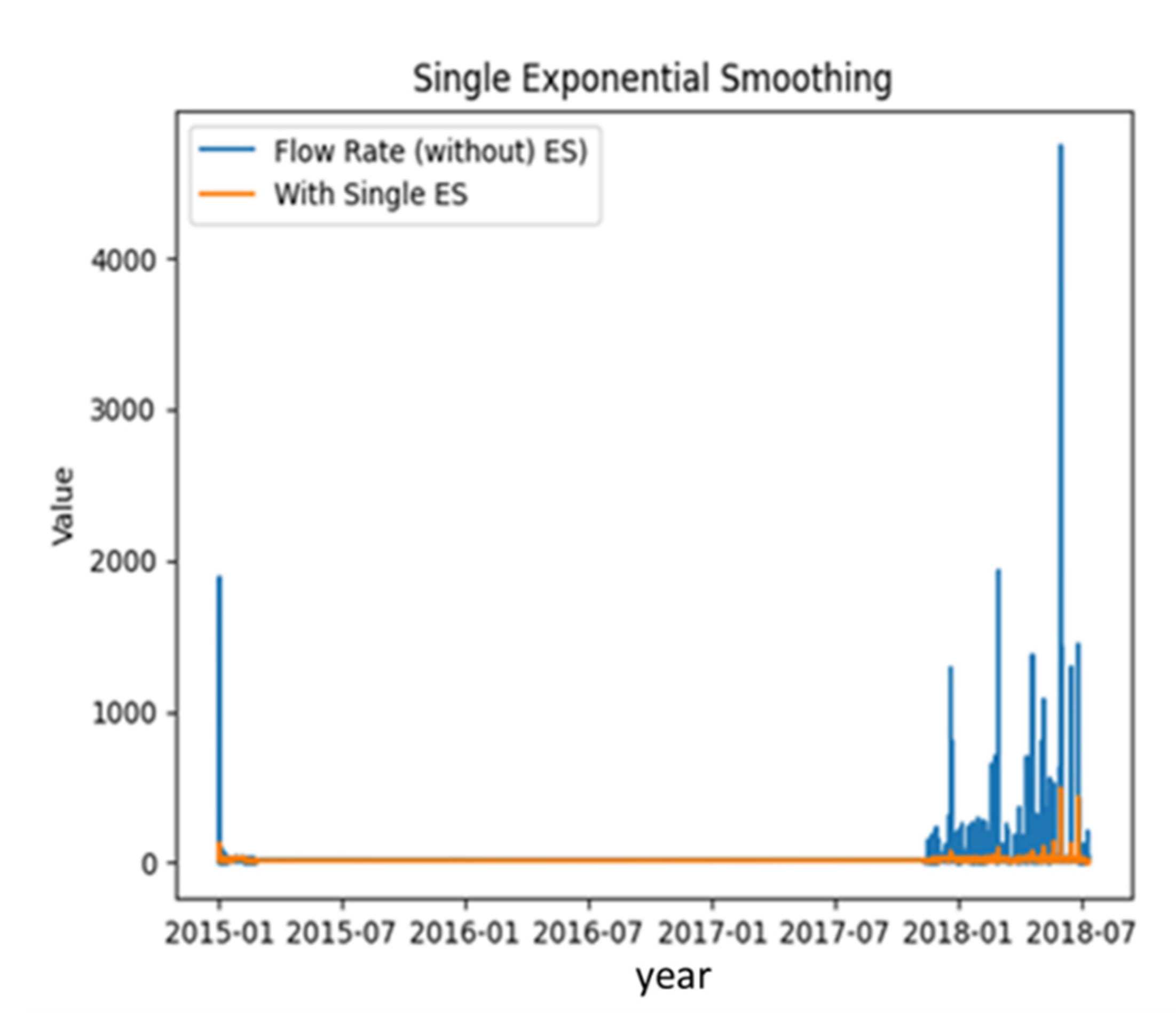
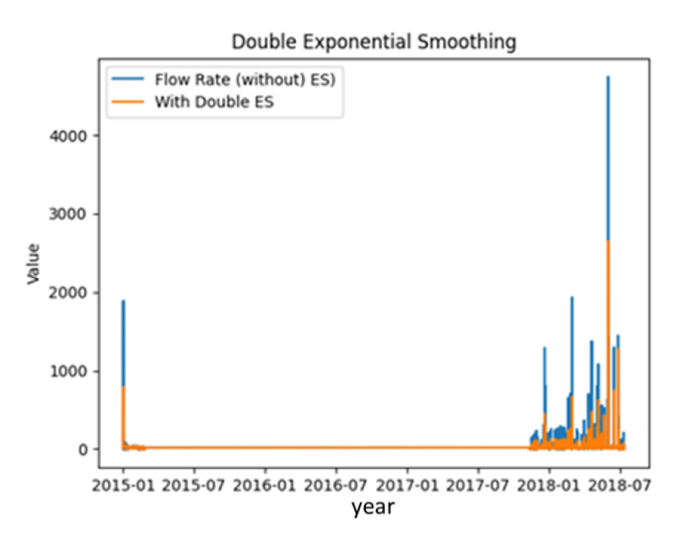
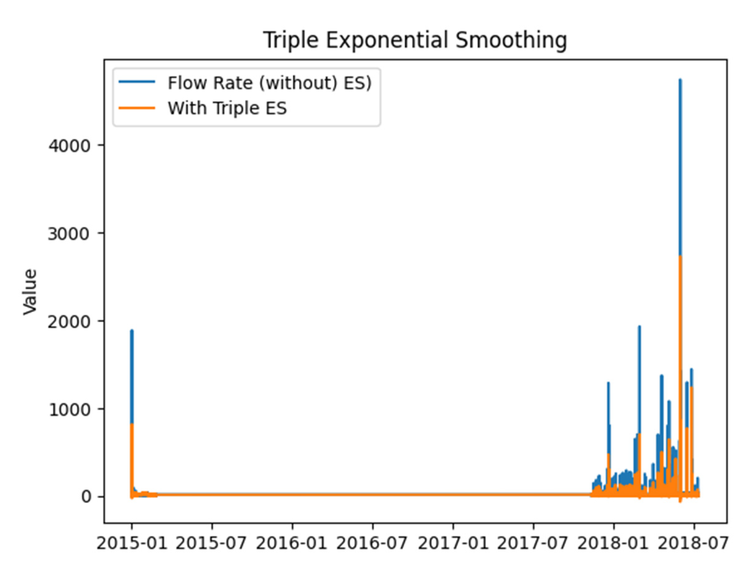
Figure 7,
Figure 8 and
Figure 9 show the results of the three methods on the same dataset.
Figure 7 and
Figure 8 show the single and double exponential smoothing methods that cannot solve seasonality in the dataset. The double exponential smoothing method can solve the trend challenge by using the trend constant. However, the seasonality problem cannot be solved because the method does not contain the seasonality parameter.
Compared with the single and double exponential smoothing methods, the triple exponential smoothing method, as shown in
Figure 9, solved the seasonality problem, making it a better choice for the data smoothing task.
Sub-Saharan African rural villages depend on solar-powered water withdrawal taps for a clean domestic water supply [
25]. However, these inadequate solar-powered taps sometimes failure and typically cause a shortage in the water supply. The result obtained from this research aid in ensuring a sustainable regime that will guarantees consistent water supply for the growing rural community.
5. Conclusions
The interest of this paper is to develop a missing data imputation method to correct missing data in a time series dataset. The aim was to prepare our dataset for failure prediction. Therefore, the degree of missingness, the time (i.e., the computational time) required to prepare (preprocess) the dataset and the quantity of dataset under investigation must be considered in deciding an appropriate approach for the data preparation task.
In order to achieve our aim, we used the BiGRU-enabled GAN generator network to generate newly synthesised samples similar to our dataset. At the same time, our model enabled the discriminator network to distinguish between the synthesised and original datasets. This distinction normally comes with some errors, but the RMSE helped the BiGRU by minimising the error. The results show that the proposed BiGAN achieved the lowest RMSE score, making it a better choice for missing data imputation.
In this paper, we considered time a crucial factor and that consideration influenced the data preparation technique proposed. The e-tap dataset is a large dataset with many missing values. As such, it requires a method that can salvage some of the implementation time to develop an efficient failure prediction model that works in real time. In order to achieve time efficiency for the model, the bidirectional GRU was adopted and fused with the GAN techniques.
After data imputation, the dataset still exhibited some seasonality and trends, which needed to be corrected before the dataset could be used for effective and unbiased failure prediction. Therefore, the triple exponential smoothing method was chosen to solve the seasonality and trends in the dataset. This method helped to further prepare the dataset for efficient failure prediction model development. With this proposed method, we can conclude that the BiGAN is a better choice for missing data imputation involving large datasets.


