Article

Machine Learning-Based Flexural Capacity Prediction of Corroded RC Beams with an Efficient and User-Friendly Tool

by
Abdelrahman Abushanab
1,
Tadesse Gemeda Wakjira
2,* and
Wael Alnahhal
1
1
Department of Civil and Architectural Engineering, Qatar University, Doha 2713, Qatar
2
School of Engineering, University of British Columbia, Kelowna, BC V1V 1V7, Canada
*
Author to whom correspondence should be addressed.
Sustainability 2023, 15(6), 4824; https://doi.org/10.3390/su15064824
Submission received: 17 February 2023 / Revised: 6 March 2023 / Accepted: 7 March 2023 / Published: 8 March 2023
(This article belongs to the Special Issue Robust and Resilient Structures for Sustainable Development)

Abstract

:
Steel corrosion poses a serious threat to the structural performance of reinforced concrete (RC) structures. Thus, this study evaluates the flexural capacity of RC beams through machine learning (ML)-based techniques with six parameters used as input features: beam width, beam effective depth, concrete compressive strength, reinforcement ratio, reinforcement yield strength, and corrosion level. Four single and ensemble ML models are evaluated; namely, decision tree, support vector machine, adaptive boosting, and gradient boosting. Hyperparameters of each model were optimized using grid search and K-fold cross-validation with root mean squared error used as the performance index. The predictive performance of each model was assessed using four statistical performance metrics. The analysis results demonstrated that the decision tree model exhibited overfitting and limited generalization ability. The adaptive boosting model also had a slight overfitting issue. In addition, the support vector machine reported comparable accuracy to that of adaptive boosting. Conversely, the proposed gradient boosting ensemble model achieved the best performance with strong generalization ability, as indicated by its lowest mean absolute error of 2.78 kN.m, mean absolute percent error of 13.40%, and root mean squared error of 3.56 kN.m, and the highest coefficient of determination of 97.30% on the test dataset. The optimized gradient boosting model has been deployed into a graphical user interface, allowing for practical implementation of the model and enabling fast, efficient, and intelligent prediction of the flexural capacity of corroded RC beams.

1. Introduction

Steel corrosion puts reinforced concrete (RC) structures at a risk of severe premature deterioration due to its association with drastic damages, lifespan shortening, and costly maintenance [1]. The generation of steel corrosion in RC members occurs mostly in aggressive marine environments [1]. The global maintenance and rehabilitation costs of corroded RC structures are estimated at USD 100 billion [2]. Additional costs estimated at 10 times the maintenance cost are assigned to road closures, traffic diversions, and public disturbance, harshly affecting the countries’ economy and population’s comfort [3]. Therefore, investigation related to the residual strength of RC members is currently of significant interest to researchers worldwide.
Constructing RC structures in corrosive mediums without considering corrosion susceptibility can lead to detrimental effects on the elements’ reinforcement, concrete surface, and bond strength with steel bars, which subsequently degrade the bending capacity of the members [4,5,6]. Particularly, corrosion decreases the cross-sectional area of the rebars, thereby affecting the overall structural performance of the buildings [4]. In addition, corrosion products expand the volume of reinforcement and therefore crack and spall of the concrete cover and, in turn, reduce the effective height and cross-sectional reinforcement area of the RC members [5]. Moreover, the corrosion products generated at the concrete-reinforcement interface reduce the adhesion of the composite and deteriorate the bars’ ribs and consequently decrease the bond strength, which can worsen the stress transfer mechanism between concrete and reinforcement and tension stiffening of the corroded elements [6].
Several research studies have explored the potential risk and countermeasures of steel corrosion on the flexural behavior of RC beams and slabs [7,8,9,10,11]. Three types of corroded specimens were considered in the previous studies; namely, specimens exposed to natural corrosive environments, specimens extracted from existing structures, and specimens corroded using the impressed current/voltage techniques with a target corrosion level (CL). Whereas the first and second specimen types might not be easy to prepare and test, the third method is the easiest and fastest for laboratory investigation [7,8,9,10]. Almusallam et al. [7] reported that RC slabs with a CL of 5% had a reduction of 25% in the flexural strength. However, the drop in the flexural capacity was increased to 60% when the CL increased to 25%. Rodriguez et al. [8] pointed out that the structural capacity of corroded RC beams is reduced due to the spalling and cracking of concrete. Mangat and Elgarf [9] demonstrated that the degradation of the flexural strength is primarily caused by a steel-concrete bond deterioration. Huang and Yang [10] suggested that the reduction of the ultimate strength of corroded RC beams is related to the concrete properties and concrete cracks.
Few analytical models are currently available to evaluate the residual flexural capacity of corroded RC beams [12,13]. Likewise, limited studies have been involved to predict the residual flexural capacity of corroded RC beams from a set of numerical data [2]. Even though the established analytical and numerical models have incorporated factors such as corrosion level, bond strength, and beams’ geometries, they still suffer from a lack of prediction accuracy. This is because the models are developed deterministically, based on limited levels of parameters. Therefore, it is vital to develop a more reliable and accurate model to enhance the prediction of the flexural capacity of corroded RC beams. Recently, machine learning (ML) algorithms have emerged as a popular approach for improving the accuracy of predictive models owing to their ability to identify complex and nonlinear relationships between the independent and dependent variables [14,15,16,17,18].
Previous studies have demonstrated the effectiveness of ML models in estimating the structural performance of both concrete [18,19] and steel [20] structures, resilience and livability assessment of smart cities [21], and seismic risk assessment [22]. However, there is a dearth of research employing ML-based models in predicting the flexural capacity of corroded RC beams. Thus, this study aims to evaluate the efficiency of various ML models in predicting the residual flexural capacity of corroded RC beams. A comprehensive dataset of the flexural behavior of corroded RC beams was collected from previous studies [8,12,13,23,24,25,26,27]. The dataset was then randomly split into 80% training data and 20% test data. Different single and ensemble ML models were then trained and evaluated to select the best predictive model. Finally, the most effective model was integrated into a graphical user interface (GUI) for practical implementation, allowing fast, accurate, and intelligent prediction of the flexural capacity of corroded RC beams.
The remainder of this paper is structured as follows: Section 2 presents the research significance, Section 3 presents the methodology, and Section 4 discusses the results. Lastly, in Section 5, the paper concludes by pointing out the limitations of this study and recommendations for future research.

2. Research Significance

As has been highlighted in the introduction, steel corrosion is a major threat to the flexural performance of RC beams, and there is a need to consider the corrosion effect in evaluating the residual flexural capacity of corroded RC beams. However, there is currently no available data-driven model for evaluating the flexural capacity of corroded RC beams. Therefore, the novelty of this study lies in the implementation of data-driven ML models to develop accurate predictions for the flexural capacity of corroded RC beams. Furthermore, a novel user-friendly GUI-based tool has been developed for practical implementation of the ML model, enabling fast, accurate, and intelligent prediction of the flexural capacity of corroded RC beams. The main objectives of this study are as follows:
  • To develop ML predictive models that can accurately estimate the flexural capacity of corroded RC beams.
  • To evaluate and compare the performance of various ML models using statistical indices such as mean absolute error (MAE), mean absolute percent error (MAPE), root mean squared error (RMSE), and coefficient of determination (R2) and select the most accurate and reliable predictive model.
  • To develop a graphical user interface for the best predictive model, which facilitates its practical implementation and enables fast, accurate, and intelligent prediction of the flexural capacity of corroded RC beams.

3. Material and Methods

The methodology adopted in this study is summarized in Figure 1 and discussed in the following subsections.

3.1. Research Database

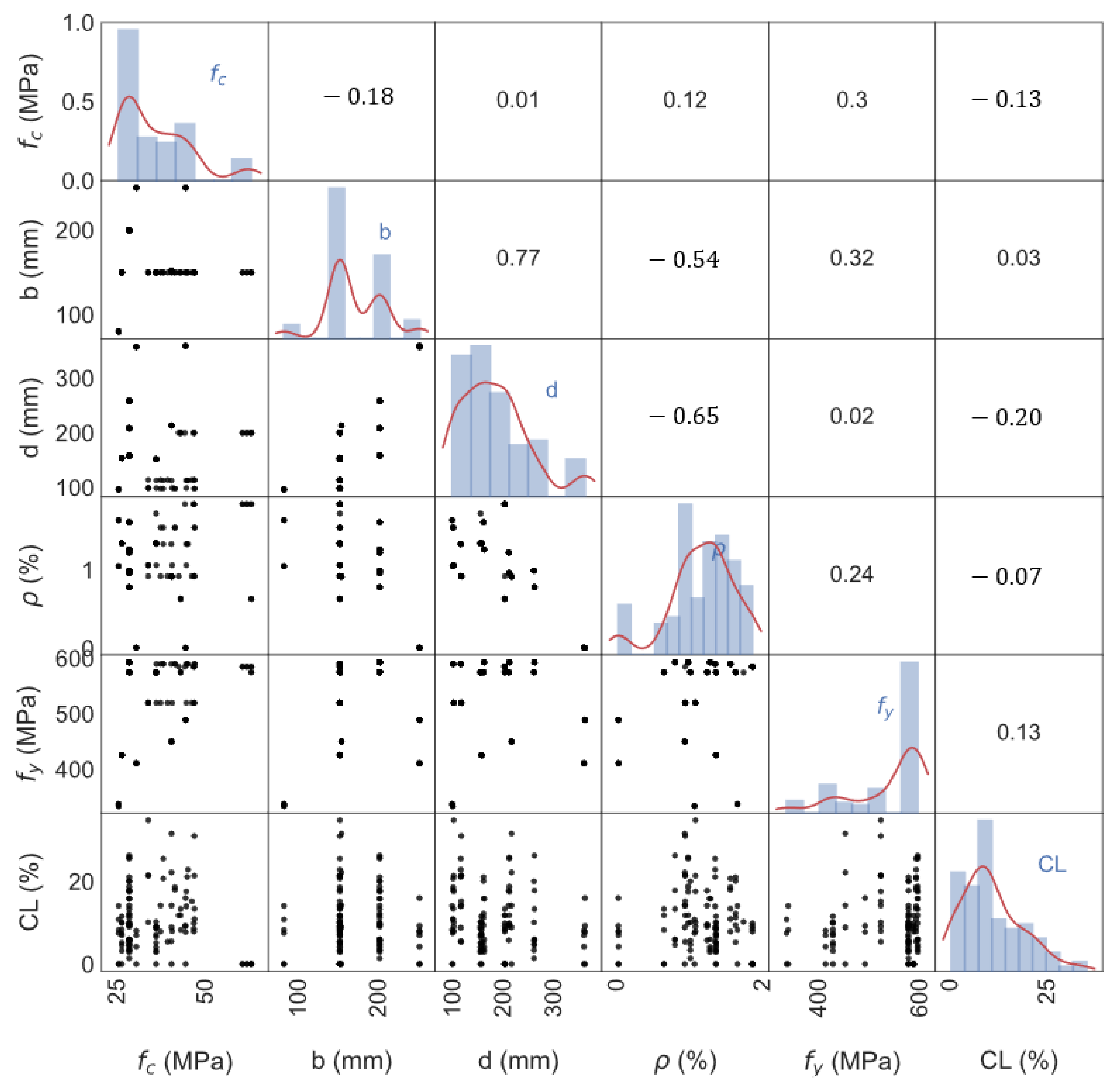
The first step involved compiling a database of the flexural capacity of corroded RC beams, as illustrated in Figure 1. The database developed in this study consisted of the flexural capacity of 115 corroded RC beams obtained from the published literature [8,12,13,23,24,25,26,27], particularly 16 sets from Rodriguez et al. [8], 24 sets from Azad et al. [12], 36 sets from Azad et al. [13], 5 sets from El Maaddawy et al. [23], 20 sets from Xia et al. [24], 11 sets from Wang et al. [25], 6 sets from Tan and Nguyen [26], and 8 sets from Yalciner et al. [27]. It is worth noting that all the beams in the constructed database were subjected to accelerated corrosion. As illustrated in Figure 2, the database employed included 6 input features with a wide range of concrete and reinforcement characteristics, beam geometry, and mass losses of corroded bars due to the chloride ingress. The input parameters were the beam width (b), beam effective depth (d), concrete compressive strength ( f c ) , reinforcement ratio (ρ), reinforcement yield strength (fy), and corrosion level (CL).
Figure 2 displays the statistical characteristics of the input parameters, which can be summarized as follows:
  • Concrete compressive strength: the beams considered in this database had concrete compressive strength in the range of 25 MPa 62.62 MPa.
  • Beam geometry: the beams’ widths ranged between 80 mm and 250 mm, and the beams’ effective depths were in the range of 96 mm to 359 mm.
  • Reinforcement characteristics: the yield strength of steel reinforcement varied from 334 MPa to 593 MPa.
  • Reinforcement ratio: the beams’ reinforcement ratios ranged between 0.0045% and 1.84%.
  • Mass loss: the mass loss of the beams, which was expressed as the CL, varied between 0% and 34.8%.
Moreover, statistical measures in terms of the histogram distribution for each parameter and Pearson correlation coefficient (r) between the inputs are provided in a 6 × 6 matrix in Figure 2. In addition, the matrix illustrates the scatter plots of the variables in the upper and lower triangular matrices.
In the subsequent step, the compiled database was randomly split into training and test datasets, comprising 80% and 20% of the complete dataset, respectively. These datasets were then employed to train and evaluate various machine learning models, as depicted in Figure 1. A brief background of the ML models is provided in the following subsection.

3.2. Machine Learning Models

This study aimed to identify the most accurate and reliable predictive model for estimating the flexural capacity of corroded RC beams, as depicted in Figure 1, by establishing four ML models. Initially, single ML models such as support vector machine (SVM) and decision tree (DT) were developed to predict the flexural capacity of corroded RC beams. However, due to the complex nature of flexural behavior in RC beams with corrosion, ensemble ML models, specifically adaptive boosting (ADB) and gradient boosting (GB), were employed to improve the predictive capability and reduce the error of the ML models.

3.2.1. Single ML Models

Support Vector Machine

SVM is a supervised ML algorithm that can be used for regression and classification problems. The input features in the SVM algorithm are mapped to a high-dimensional space using a fitting procedure. For N number of training datasets x i , y i i = 1 N ϵ R Q × R , SVM estimates the parameters of a regression function (Equation (1)) by minimizing the regularized risk function (Equation (2)), which is conditioned by Equations (3)–(5) [28].
f x = w . ϕ x + b
τ w , ξ , ξ * = 1 2 w 2 + C 1 2 i = 1 n ξ i + ξ i * ,   i = 1 , 2 , , n
w . ϕ x + b y i ε + ξ i ,   i = 1 , 2 , , n
y i w . ϕ x + b   ε + ξ i * ,   i = 1 , 2 , , n
f x = w . ϕ x + b
ξ i , ξ i * 0  
where ξ i   and ξ i *   are the slack variables, w is the weight vector, b is the bias, ε is the Vapnik’s insensitive loss, and C is the regularization parameter.
The prediction of the SVM algorithm is achieved as per Equation (7) [29,30]:
f x = i ϵ S V ( α i α i * ) K x i , x + b   s u b j e c t   t o   α i , α i *   ϵ 0 , C
where SV stands for support vectors, K x i , x is the kernel function, b is a bias, C is the regularization parameters, and α i and α i * are the Lagrange multipliers of the lower and upper SV, respectively.

Decision Tree

The DT algorithm is a widely used supervised algorithm and is considered the base learner for many advanced algorithms. It is a non-parametric algorithm that can be used for classification and regression analyses by constructing a flowchart-like structure [31]. The algorithm is known for its ease of data preprocessing, visualization, and interpretation, as well as being unaffected by outliers. The DT algorithm is composed of three main nodes: root, internal, and leaf. The root node identifies the main characteristic of the data, and the internal and leaf nodes are branched from the root nodes. Each internal node represents a test on an attribute, and the leaf node covers the response prediction.
The tree predictor is developed by iteratively partitioning the input space N into K distinct subspaces R 1 ,   ,   R K , in which aggregation occurs for observations with similar targets. This is accomplished by using the Gini Index and mean squared error for classification and regression problems, respectively [32]. A minimal cost-complexity pruning algorithm is then utilized to trim the tree and avoid overfitting the DT model [32]. The DT model can be defined as per Equation (8):
h x = k = 0 K b k I x ϵ R k  
where R k is the kth distinct subspace, b k is the prediction of the subspace R k , and I x ϵ R k is the indicator function ( I x ϵ R k = 1 when x R k ).
Single DT algorithms have weaknesses in terms of data generalization, high variance, and bias. To address this problem, ensemble models are employed, as discussed in the following subsection.

3.2.2. Ensemble ML Models

Ensemble algorithms are a more advanced ML technique that seeks to reduce bias and variance and improve the prediction performance of single models. This is accomplished by sequentially combining multiple weak learners (in this study, DT) to create a single strong learner. Boosting ensembles are the most frequently used ensemble models. Details of the boosting ensembles are provided in the following subsections.

Adaptive Boosting

The first boosting algorithm to be developed was ADB. The ADB algorithm trains and reweighs weak learners (DT in this study) iteratively over multiple training rounds to correlate inputs (X) with the output (Y) parameter. The weighting vector is adjusted during each training process to account for misclassified instances from previous iterations (excluding the first iteration). Given a training dataset of Z samples in Equation (9), the ADB algorithm iteratively trains several base learners ft(X) to construct a single improved model F(X), see Equation (10):
X ,   Y = X i ,   Y i i = 1 Z  
where X i represents the ith input parameters and Y i is the ith response variable in the training dataset.
F X = k = 1 K G w k f k X  
where K is the total number of base learners and w k is the weight of kth learner.
During the first iteration, the weight is uniformly distributed among the weak learners with a constant weight of w 1 ,   i = 1 / Z ,   i [33]. Subsequently, the weighting process of the observations is readjusted by assigning higher weight to the incorrectly predicted observations in the initial iteration. The weight distribution for training step t is adjusted according to Equation (11), where βt ∈ [0, 1] is the parameter related to the distribution update (Equation (12)), and L k ¯ is the average loss function (Equation (13)). A linear loss function was also used in this study to assess the performance of the base learner, as shown in Equation (14):
w k + 1 ,   i = w k ,   i β k 1 L k , i i = 1 N w k ,   i β k 1 L k , i
β k = L k ¯ 1 L k ¯
L k ¯ = i = 1 N D k ,   i   L k ,   i
L k ,   i = Y k f k , i X i max Y i f k , i X i , i = 1 ,   ,   N

Gradient Boosting

The gradient boosting (GB) algorithm is another type of boosting algorithms that combines multiple base learners (DT in this study) sequentially and accumulates the results in an additive model. The mathematical expression of the GB algorithm is presented in Equation (15):
F K x = k = 0 K f k x
where K is the number of base learners and f k is all possible base learner (DT in this study).
The GB algorithm utilizes the gradient descent method in each sequential iteration to construct new trees from the previous base learners and reduce the loss function. The GB model is initiated in the first iteration using a constant value as per Equation (16) to reduce the loss. Following the first iteration, the GBDT model fits a new DT base learner h k X at each iteration t, as shown in Equation (17), to the negative gradient descent ( r i ,   k ) or pseudo-residuals of the previous learner in the sequence, i.e., training set x i ,   r i ,   k   i = 1 N , as presented in Equation (18), which is obtained by solving Equation (19):
F o X = a r g   m i n γ i = 1 N L Y i , Y ^ i  
F k X = F k 1 X + γ k h k X ,   f o r   k = 1 , ,   K  
r i ,   k = L Y i , F X i   F X i F X = F k 1 X     ,   f o r   i = 1 ,   ,   N  
γ k = a r g   m i n γ i = 1 N L Y i , F k 1 X i + γ h k X i
in which, L · and γ k are the training loss and multiplier, respectively.

4. Results and Discussion

4.1. Hyperparameter Optimization Results

As previously mentioned and depicted in Figure 1, the database was randomly divided into training and testing datasets. The hyperparameters of the models were optimized using the grid search technique, which involves searching through a predefined grid of hyperparameters to find the optimal values of the hyperparameters. Additionally, to address overfitting during the training process, the widely used K-fold cross-validation method was employed. This method divides the dataset into k subsets or folds, trains the model on k-1 folds, and validates it on the remaining one fold. This process is repeated k times, where each subset of the data serves as both the validation and training set. The cross-validated model’s performance is then calculated as the average performance across the K validation sets. In this study, the widely used 10-fold cross-validation technique (K = 10) was employed.
The optimization process was performed using RMSE as the evaluation metric. The results of the hyperparameter optimization are presented in Table 1. The optimized SVM utilized a radial basis function (RBF) kernel, with a regularization parameter (C) set to 30 and an epsilon value of 10−5. The decision tree was fine-tuned by optimizing its hyperparameters, resulting in a maximum tree depth of five, a maximum of four randomly chosen input features, a minimum sample requirement of two for splitting internal nodes, and a minimum sample requirement of one for leaf nodes.
The AdaBoost model was optimized with the number of estimators set to 10, a learning rate of 0.15, and a decision tree as the base learner. For the base decision tree, the maximum tree depth was set to ten, the maximum number of randomly selected input features was three, a minimum of two samples were required to split an internal node, and the minimum number of samples at a leaf node was one, as presented in Table 1. The optimized gradient boosting model used twenty base learners, with a maximum tree depth of five, 30% of the samples used for fitting each base learner, and a learning rate set to 0.25, as listed in Table 1.

4.2. Model Performance

Figure 3 presents the scatter plots of the experimental (Mexp) and predicted (Mpred) flexural capacities based on the optimized ML models. The green line in the scatter plots shows an ideal match between the predicted and experimental flexural capacities. The results in Figure 3 demonstrate that all ML models achieved high predictive accuracy on the training set, evidenced by their high R2, which ranged between 96.8% for DT to 99.8% for ADB. Nevertheless, the predictive accuracy of the models varied markedly on the test set, especially in the case of the DT model, which achieved a low R2 of 73.3% (Figure 3c). The weak prediction of the DT model indicates overfitting and a lack of generalization ability of the algorithm. Moreover, SVM exhibited the highest accurate prediction among the single ML models with an R2 of 97.3% and 90.2% for training and test sets, respectively. It can also be seen from Figure 3c,d that integrating decision trees into an ensemble framework, such as ADB and GB models, substantially improved the prediction accuracy and generalization capability of the models. This is evidenced by the improvement achieved in the R2 of both ensemble models on both databases. In principle, the graphical comparison showed that the accuracy of the ADB model was comparable to that of the SVM on the test database, as evidenced by the close values of R2 on the test datasets. However, ADB prediction achieved better distribution of the data, as the majority of the data was closer to the error bounds compared to SVM prediction. Furthermore, GB prediction exhibited the highest prediction accuracy compared to all models. This could be exemplified by the R2 (97.3%) of the test set, which was 7.87%, 32.74%, and 7.51% higher than the SVM, DT, and ADB models, respectively. The outperformance of the GB prediction implies the effectiveness of the GB algorithm in predicting the flexural capacity of corroded RC beams. The performance of the models is further investigated and compared in the following subsection.

4.3. Comparison of Predictive Models

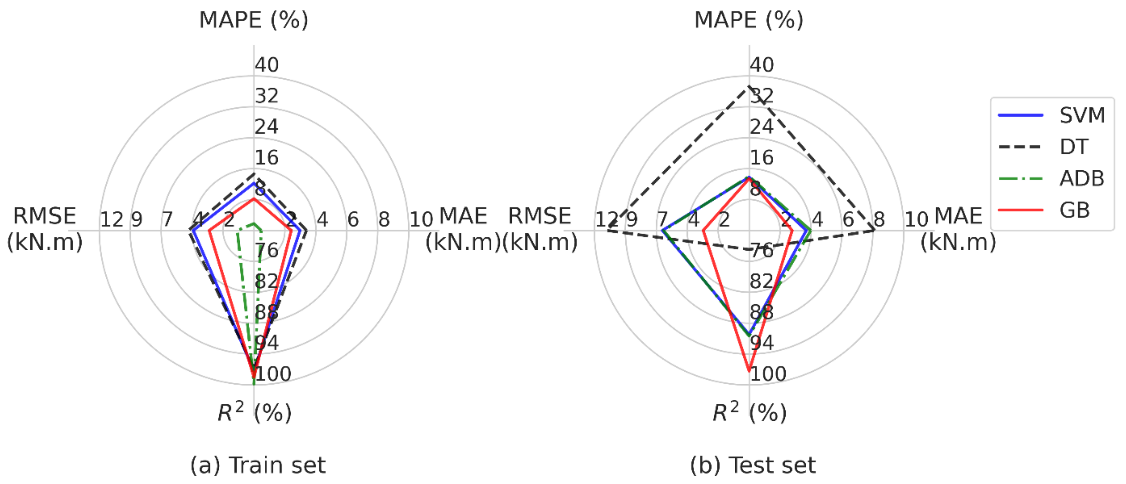
The efficiency of the fine-tuned ML models was rigorously evaluated by utilizing four essential statistical performance indicators: MAE, MAPE, RMSE, and R2. The evaluation results of the models are summarized in Table 2. Furthermore, Figure 4 presents the performance metrics in spider plots to enable visualization and comparison of the performance of each model against the others. Based on the results presented in Table 2, DT exhibited the least accuracy and a clear case of overfitting, owing to the high statistical error and low R2. In particular, the DT recorded MAE of 3.39 kN.m and 8.12 kN.m, MAPE of 14.61% and 37.29%, and RMSE of 5.09 kN and 11.05 kN on the training and test sets, respectively. In addition, the R2 of the DT on the training set was as high as 96.8%, whereas on the test set, the DT model exhibited a significantly low R2 of 73.70%. It can also be seen in Figure 4 that the spider plot of the DT prediction on the test set significantly diverged toward a higher MAPE error. This indicates that the DT model is not able to generalize well to new data and suffers from overfitting. Furthermore, it could be seen that the SVM model outperformed the DT model with a higher R2 of 90.2% on the test dataset compared to the DT’s R2 of 73.7%, as listed in Table 2. The SVM model also exhibited lower MAE, MAPE, and RMSE on test and training datasets compared to the DT model. The SVM has 54.43%, 63.02%, and 39.10% lower MAE, MAPE, and RMSE on the test dataset, respectively, compared to the DT model. The improved accuracy of the SVM prediction can also be revealed in Figure 4, where the spider plot showed a lower error compared to the DT prediction.
On the other hand, the results showed that the ADB model has an MAE of 0.47 kN.m and 3.99 kN.m, MAPE of 1.78% and 13.98%, and RMSE of 1.3 kN.m and 6.64 kN.m on the training and test sets, respectively. Even though the ADB model recorded a high R2 of 99.8% on the training set, the predictive performance of the model was significantly dropped on the test set, evidenced by the R2, which was reduced to 90.50%. This suggests that the ADB model may also be suffering from some overfitting and generalization capability. The GB demonstrated higher performance than the ADB model, with a lower error on both training and testing datasets, as can be seen in Figure 4 and Table 2. The R2 of the GB model was recorded at 98.5% and 97.30% on the training and test sets, respectively. Furthermore, the GB prediction achieved MAE and RMSE of 2.78 and 3.56 on the test set, which is about 30.33% and 46.39% lower than those of the ADB prediction, respectively. This implies that the GB model fits the data well and performs well on both the training and test sets. Overall, the GB model exhibited the highest prediction accuracy with the highest R2 and lowest error on the test sets among the investigated models. Thus, it can be used effectively to accurately predict the flexural capacity of corroded RC beams.

4.4. An Intelligent Prediction Tool with Fast and Accurate Results

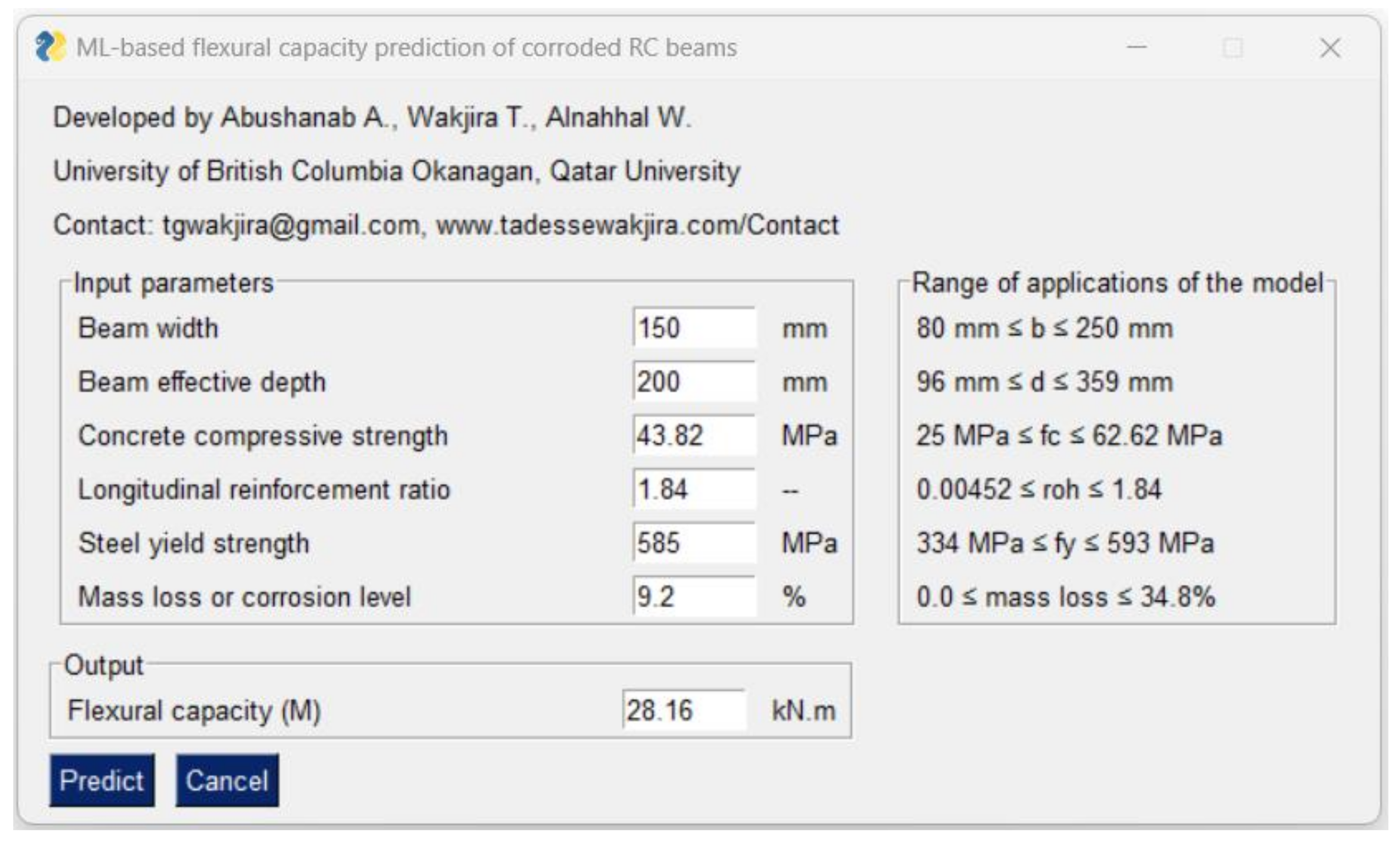
In an earlier discussion, it was observed that the proposed GB model had excellent potential for predicting the flexural capacity of corroded RC beams. However, to make the model practically useful, there was a need to develop a GUI-based software that would be user-friendly. Therefore, a GUI software was developed for the GB model using Python programming language, and a screenshot of the tool is shown in Figure 5. The developed GUI tool is available for download via the following link: https://github.com/twakjira/GUI-corrodedRCbeam-capacity, accessed on 5 March 2023. Figure 5 provides a visual representation of the proposed model’s range of applicability. By utilizing this GUI software, we were able to accurately predict the flexural capacity of corroded beam in specimen B10-05. As shown in Figure 5, the predicted shear capacity of this specimen was 28.16 kN.m, which is highly consistent with the corresponding experimental value (Mexp = 29 kN.m [8]).

5. Conclusions

This paper presents machine learning-based predictive models for estimating the flexural capacity of reinforced concrete beams with corroded bars. Four different ML models were established; namely, SVM, DT, ADB, and GB. The database was preprocessed and randomly divided into training and test datasets using an 80/20 training/test split ratio. The hyperparameters of the models were optimized using grid search and K-fold cross-validation. Four commonly used performance metrics, including MAE, MAPE, RMSE, and R2, were employed to evaluate the predictive performance of the models.
The following conclusions can be drawn from the results of this study:
  • The DT model exhibited overfitting, with significantly higher values on the test set compared to the training set, indicating that it may not generalize well to new data. Specifically, on the training set, it achieved an MAE of 3.39 kN.m, MAPE of 14.61%, RMSE of 5.09 kN.m, and R2 of 96.8%. However, it showed overfitting with an MAE of 8.12 kN.m, MAPE of 37.29%, RMSE of 11.05 kN.m, and R2 of 73.70% on the test dataset.
  • The SVM model achieved a relatively good performance with an MAE of 3.70 kN.m, MAPE of 13.79%, RMSE of 6.73 kN.m, and R2 of 90.20% on the test set.
  • The ADB model showed high performance on the training set with an MAE of 0.47 kN.m, MAPE of 1.78%, RMSE of 1.30 kN.m, and R2 of 99.8%. However, it experienced a significant drop in the predictive performance on the test set, indicating some overfitting and less generalization capability.
  • The GB model outperformed the other models with the lowest MAE of 2.78 kN.m, MAPE of 13.40%, and RMSE of 3.56 kN.m, and the highest R2 of 97.30% on the test set. Consequently, the developed gradient boosting model can be used to accurately predict the flexural capacity of corroded RC beams.
Finally, a user-friendly intelligent GUI-based tool has been developed to enable fast and accurate prediction of the flexural capacity of corroded RC beams, thus facilitating the practical implementation of the developed machine learning model. Further research is recommended to focus on the shear capacity of corroded RC beams using machine learning models. Additionally, future research can investigate the failure mode of RC corroded beams and develop classification-based machine learning models to predict the failure modes of the beams.

Author Contributions

Conceptualization, A.A. and T.G.W.; Methodology, A.A., T.G.W. and W.A.; Software, A.A. and T.G.W.; Validation, A.A., T.G.W. and W.A.; Formal analysis, A.A. and T.G.W.; Investigation, A.A. and T.G.W.; Data curation, A.A. and T.G.W.; Writing—original draft, A.A. and T.G.W.; Writing—review & editing, A.A., T.G.W. and W.A.; Visualization, A.A. and T.G.W. All authors have read and agreed to the published version of the manuscript.

Funding

This research received no external funding.

Institutional Review Board Statement

Not applicable.

Informed Consent Statement

Not applicable.

Data Availability Statement

Data will be made available upon request.

Acknowledgments

This publication was made possible by GSRA grant GSRA6-1-0509-19022 from the Qatar National Research Fund (QNRF, a member of Qatar Foundation).

Conflicts of Interest

The authors declare no conflict of interest.

References

  1. Abushanab, A.; Alnahhal, W.; Farraj, M. Structural Performance and Moment Redistribution of Basalt FRC Continuous Beams Reinforced with Basalt FRP Bars. Eng. Struct. 2021, 240, 112390. [Google Scholar] [CrossRef]
  2. Peng, J.; Yan, G.; Zandi, Y.; Sadighi Agdas, A.; Pourrostam, T.; Ezz El-Arab, I.; Denic, N.; Nesic, Z.; Cirkovic, B.; Amine Khadimallah, M. Prediction and Optimization of the Flexural Behavior of Corroded Concrete Beams Using Adaptive Neuro Fuzzy Inference System. Structures 2022, 43, 200–208. [Google Scholar] [CrossRef]
  3. Basaran, B. Effect of Steel–FRP Ratio and FRP Wrapping Layers on Tensile Properties of Glass FRP-Wrapped Ribbed Steel Reinforcing Bars. Mater. Struct. 2021, 54, 188. [Google Scholar] [CrossRef]
  4. Jnaid, F.; Aboutaha, R.S. Residual Flexural Strength of Corroded Reinforced Concrete Beams. Eng. Struct. 2016, 119, 198–216. [Google Scholar] [CrossRef]
  5. Malumbela, G.; Moyo, P.; Alexander, M. Behaviour of RC Beams Corroded under Sustained Service Loads. Constr. Build. Mater. 2009, 23, 3346–3351. [Google Scholar] [CrossRef]
  6. Imperatore, S.; Rinaldi, Z.; Spagnuolo, S. Influence of Corrosion on the Experimental Behaviour of R.C. Ties. Eng. Struct. 2019, 198, 109458. [Google Scholar] [CrossRef]
  7. Almusallam, A.A.; Al-Gahtani, A.S.; Aziz, A.R.; Dakhil, F.H. Rasheeduzzafar Effect of Reinforcement Corrosion on Flexural Behavior of Concrete Slabs. J. Mater. Civ. Eng. 1996, 8, 123–127. [Google Scholar] [CrossRef]
  8. Rodriguez, J.; Ortega, L.; Casal, J. Load Carrying Capacity of Concrete Structures with Corroded Reinforcement. Constr. Build. Mater. 1997, 11, 239–248. [Google Scholar] [CrossRef]
  9. Mangat, P.S.; Elgarf, M.S. Flexural Strength of Concrete Beams with Corroding Reinforcement. ACI Struct. J. 1999, 96, 149–158. [Google Scholar] [CrossRef]
  10. Huang, R.; Yang, C.C. Condition Assessment of Reinforced Concrete Beams Relative to Reinforcement Corrosion. Cem. Concr. Compos. 1997, 19, 131–137. [Google Scholar] [CrossRef]
  11. Abushanab, A.; Alnahhal, W.; Farraj, M. Experimental and Finite Element Studies on the Structural Behavior of BFRC Continuous Beams Reinforced with BFRP Bars. Compos. Struct. 2021, 281, 114982. [Google Scholar] [CrossRef]
  12. Azad, A.K.; Ahmad, S.; Azher, S.A. Residual Strength of Corrosion-Damaged Reinforced Concrete Beams. ACI Mater. J. 2007, 104, 40–47. [Google Scholar]
  13. Azad, A.K.; Ahmad, S.; Al-Gohi, B.H.A. Flexural Strength of Corroded Reinforced Concrete Beams. Mag. Concr. Res. 2010, 62, 405–414. [Google Scholar] [CrossRef]
  14. Cai, B.; Pan, G.; Fu, F. Prediction of the Postfire Flexural Capacity of RC Beam Using GA-BPNN Machine Learning. J. Perform. Constr. Facil. 2020, 34, 04020105. [Google Scholar] [CrossRef]
  15. Cao, W.; Wang, A.; Yu, D.; Liu, S.; Hou, W. Establishment and Implementation of an Asphalt Pavement Recycling Decision System Based on the Analytic Hierarchy Process. Resour. Conserv. Recycl. 2019, 149, 738–749. [Google Scholar] [CrossRef]
  16. Solhmirzaei, R.; Salehi, H.; Kodur, V.; Naser, M.Z. Machine Learning Framework for Predicting Failure Mode and Shear Capacity of Ultra High Performance Concrete Beams. Eng. Struct. 2020, 224, 111221. [Google Scholar] [CrossRef]
  17. Fu, B.; Chen, S.-Z.; Liu, X.-R.; Feng, D.-C. A Probabilistic Bond Strength Model for Corroded Reinforced Concrete Based on Weighted Averaging of Non-Fine-Tuned Machine Learning Models. Constr. Build. Mater. 2022, 318, 125767. [Google Scholar] [CrossRef]
  18. Wakjira, T.G.; Abushanab, A.; Ebead, U.; Alnahhal, W. FAI: Fast, Accurate, and Intelligent Approach and Prediction Tool for Flexural Capacity of FRP-RC Beams Based on Super-Learner Machine Learning Model. Mater. Today Commun. 2022, 33, 104461. [Google Scholar] [CrossRef]
  19. Truong, G.T.; Choi, K.K.; Kim, C.S. Implementation of Boosting Algorithms for Prediction of Punching Shear Strength of RC Column Footings. Structures 2022, 46, 521–538. [Google Scholar] [CrossRef]
  20. Wakjira, T.G.; Rahmzadeh, A.; Alam, M.S.; Tremblay, R. Explainable Machine Learning Based Efficient Prediction Tool for Lateral Cyclic Response of Post-Tensioned Base Rocking Steel Bridge Piers. Structures 2022, 44, 947–964. [Google Scholar] [CrossRef]
  21. Kutty, A.A.; Wakjira, T.G.; Kucukvar, M.; Abdella, G.M.; Onat, N.C. Urban Resilience and Livability Performance of European Smart Cities: A Novel Machine Learning Approach. J. Clean. Prod. 2022, 378, 134203. [Google Scholar] [CrossRef]
  22. Kourehpaz, P.; Molina Hutt, C. Machine Learning for Enhanced Regional Seismic Risk Assessments. J. Struct. Eng. 2022, 148, 04022126. [Google Scholar] [CrossRef]
  23. El Maaddawy, T.; Soudki, K.; Topper, T. Long-Term Performance of Corrosion-Damaged Reinforced Concrete Beams. ACI Struct. J. 2005, 102, 649–656. [Google Scholar] [CrossRef]
  24. Xia, J.; Jin, W.-L.; Li, L.-Y. Effect of Chloride-Induced Reinforcing Steel Corrosion on the Flexural Strength of Reinforced Concrete Beams. Mag. Concr. Res. 2012, 64, 471–485. [Google Scholar] [CrossRef]
  25. Wang, L.; Ma, Y.; Ding, W.; Zhang, J.; Liu, Y. Comparative Study of Flexural Behavior of Corroded Beams with Different Types of Steel Bars. J. Perform. Constr. Facil. 2015, 29, 04014163. [Google Scholar] [CrossRef]
  26. Tan, N.N.; Nguyen, N.D. An Experimental Study on Flexural Behavior of Corroded Reinforced Concrete Beams Using Electrochemical Accelerated Corrosion Method. J. Sci. Technol. Civ. Eng. NUCE 2019, 13, 1–11. [Google Scholar] [CrossRef]
  27. Yalciner, H.; Kumbasaroglu, A.; El-Sayed, A.K.; Balkıs, A.P.; Dogru, E.; Turan, A.I.; Karimi, A.; Kohistani, R.; Mermit, M.F.; Bicer, K. Flexural Strength of Corroded Reinforced Concrete Beams. ACI Struct. J. 2020, 117, 29–41. [Google Scholar] [CrossRef]
  28. Vapnik, V.N. The Nature of Statistical Learning Theory; Springer: New York, NY, USA, 2000; ISBN 978-1-4419-3160-3. [Google Scholar]
  29. Yu, H.; Kim, S. SVM Tutorial-Classification, Regression and Ranking. Handb. Nat. Comput. 2012, 1–4, 479–506. [Google Scholar] [CrossRef]
  30. Chang, C.; Lin, C. LIBSVM: A Library for Support Vector Machines. ACM Trans. Intell. Syst. Technol. 2011, 2, 1–27. [Google Scholar] [CrossRef]
  31. Sutton, C.D. Classification and Regression Trees, Bagging, and Boosting. Handb. Stat. 2005, 24, 303–329. [Google Scholar] [CrossRef] [Green Version]
  32. Breiman, L.; Friedman, J.H.; Olshen, R.A.; Stone, C.J. Classification and Regression Trees; Wadsworth: Belmont, CA, USA, 1984; Volume 432, p. 9. [Google Scholar]
  33. Shrestha, D.L.; Solomatine, D.P. Experiments with AdaBoost.RT: An Improved Boosting Scheme for Regression. Neural Comput. 2006, 18, 1678–1710. [Google Scholar] [CrossRef]
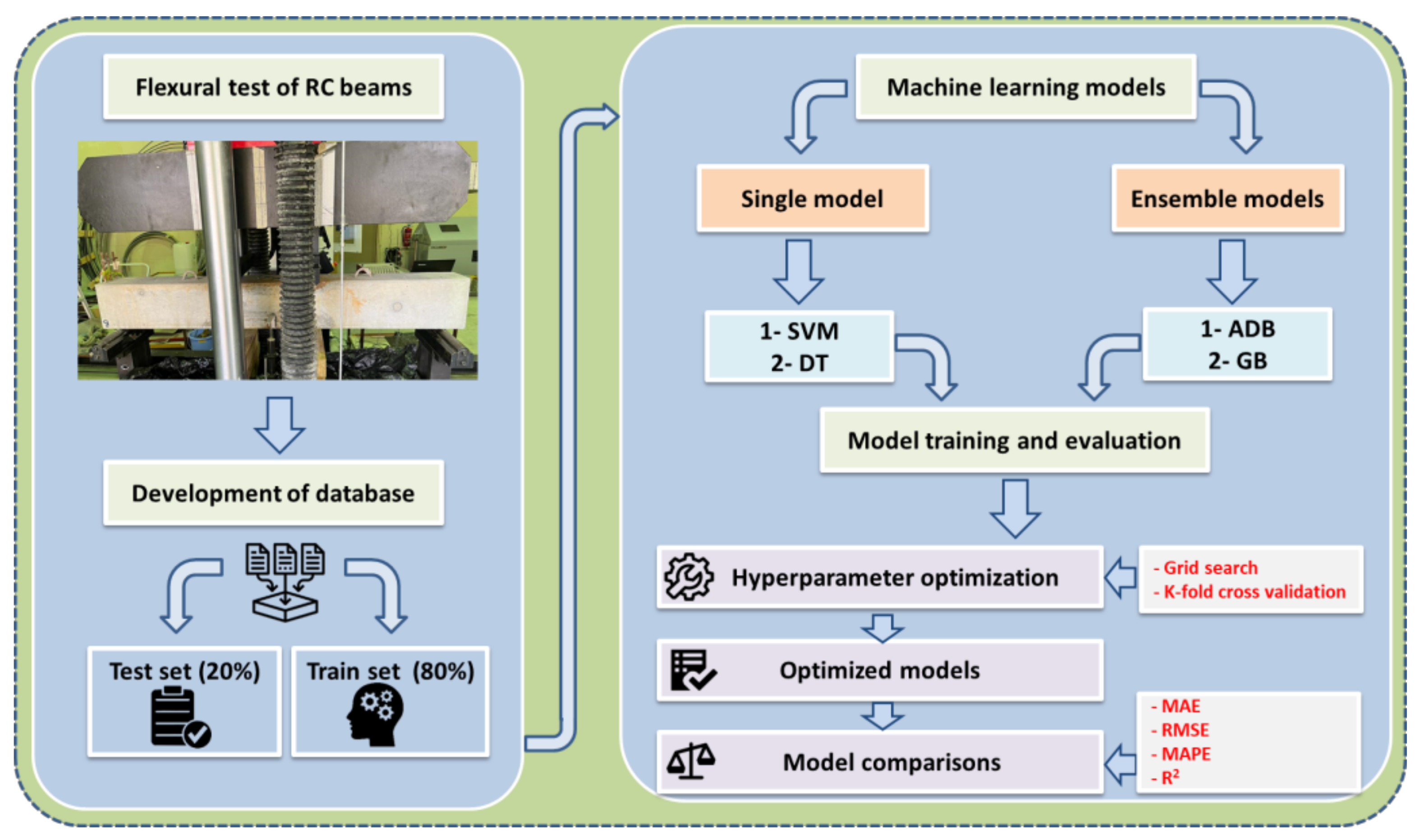
Figure 1. Flowchart of procedures adopted in this study.
Sustainability 15 04824 g001
Figure 2. Distribution of the input parameters.
Sustainability 15 04824 g002
Figure 3. Predicted versus experimental flexural capacities of the studied beams with green line indicating an ideal match between the predicted and experimental flexural capacities.
Sustainability 15 04824 g003
Figure 4. Predictive performance of the models.
Sustainability 15 04824 g004
Figure 5. GUI tool of the proposed model and flexural capacity prediction for corroded specimen 126 of Ref. [8].
Sustainability 15 04824 g005
Table 1. Optimized values of hyperparameters.
ModelTuned Hyperparameters
NameValue
Support vector machineRegularization parameter, C30
Epsilon, ε10−5
Kernel typeRBF
Decision treeMaximum tree depth5
Maximum number of randomly chosen input features4
Minimum sample required to split an internal node2
Minimum sample required at the leaf node1
Adaptive boostingNumber of estimators or base learners10
Learning rate0.15
Base learnerDecision tree
Maximum depth of base learner10
Maximum number of randomly selected input features for base learner3
Minimum sample required to split an internal node2
Minimum sample required at the leaf node1
Gradient boosting machineNumber of base learners or estimators20
Maximum depth5
Fraction of samples used to fit each base learner30%
Learning rate0.25
Table 2. Statistical measures of the models on the train and test sets.
ModelTraining SetTest Set
MAE
(kN.m)
MAPE
(%)
RMSE
(kN.m)
R2
(%)
MAE
(kN.m)
MAPE
(%)
RMSE
(kN.m)
R2
(%)
SVM2.9712.234.7197.33.7013.796.7390.20
DT3.3914.615.0996.88.1237.2911.0573.70
ADB0.471.781.399.83.9913.986.6490.50
GB2.418.243.4898.52.7813.403.5697.30
Disclaimer/Publisher’s Note: The statements, opinions and data contained in all publications are solely those of the individual author(s) and contributor(s) and not of MDPI and/or the editor(s). MDPI and/or the editor(s) disclaim responsibility for any injury to people or property resulting from any ideas, methods, instructions or products referred to in the content.