1. Introduction
In recent years, the rapid development of electronic commerce has triggered further expansion of China’s logistics market. The development of the logistics industry has taken up a large amount of resources and brought about greater environmental pollution. Traditional logistics systems have gradually lowered the development efficiency of enterprises, thus there is a demand for intelligent logistics systems. For labor-intensive, repetitive, and hazardous environments, mobile robots to replace human work have gained widespread attention, which is critical to the operational efficiency and resource consumption of modern factories and warehouses [
1].
Path planning technology is one of the key technologies to realize the intelligence of mobile robots, which refers to finding an optimal or suboptimal path from the starting point to the end point without collision in a complex spatial environment according to the set initial and target positions during the robot operation [
2]. Academically, the path planning problem for robots is divided into the path planning problem for static environments [
3] and the path planning problem for dynamic environments [
4].
Since today’s mobile robots usually use a pre-laid magnetic track to pick up goods at a fixed point, the pickup route is relatively single. When multiple mobile robots are operating at the same time, there may be different forms of collisions between them, therefore the obstacle avoidance between them needs further study. Path planning technology, as a core technology of mobile robots, is the basis and prerequisite for completing subsequent tasks. Reducing the path length of the robot and improving the path smoothness can improve efficiency, ensure driving safety, reduce robot wear and tear, improve robot life, reduce energy consumption, and improve green logistics. Therefore, it is of great economic and practical value to study the global path planning problem.
This paper creatively proposes to use the improved genetic algorithm to obtain the key turning point on the static global optimal solution, which makes good use of the advantages of the high-solving efficiency of the genetic algorithm and the multi-objective solution. The traditional genetic algorithm is improved by introducing a population fitness variance, an adaptive elite retention factor, and a regeneration operator, as well as improved adaptive selection, crossover, and mutation probabilities to avoid prematurely falling into a local optimum solution. The sum of turning angles and the number of turning points of the planned paths are added to the fitness function as smoothing indicators and the paths are further optimized by the key point extraction strategy to obtain the global optimal paths. For the traditional dynamic window approach, we improve the robustness of the dynamic obstacle avoidance of the robot and reduce the path length by improving the simulation trajectory evaluation function, the initial heading angle of each sub-node, and the adaptive adjustment of the robot motion state, which is conducive to the obstacle avoidance of robot. Finally, experiments in different scenarios verify that the path planning algorithm proposed in this paper can well carry out the global dynamic path planning that achieves both dynamic obstacle avoidance and an approximate global optimal dynamic path.
In general, the main contribution of this paper aims at the problems of redundant points, low planning efficiency, unsmooth path, and multiple turning points of the traditional genetic algorithm. In addition, problems such as the traditional dynamic window approach may have a long path in planning and cannot reach the target point in the face of “C”-shaped obstacles, thus this paper puts forward the optimization methods of the two algorithms and the fusion scheme of the optimization algorithms to realize the dynamic obstacle avoidance of the mobile robot of unknown obstacles, as well as the optimal smooth path considering that real-time obstacle avoidance is obtained.
The rest of the paper is organized as follows: In the second section of this paper, the environment model, fitness function, and constraint conditions of robot path planning are established. The third section uses the improved genetic algorithm to solve the fitness function in the second section. The fourth section combines the improved dynamic window approach (improved DWA) algorithm and genetic algorithm for path planning. The fifth section carries on the simulation experiment and the result analysis. The sixth section summarizes the research results of this paper.
2. Related Work
Mobile robots are widely used in many fields such as logistics, transportation, life services, industrial manufacturing, etc., because of their autonomous navigation and flexible movement. Path planning is an important part of autonomous navigation technology for mobile robots [
5]. It uses the robot’s various sensors to obtain environmental information in a complex environment to help the robot plan a safe and fast optimal or sub-optimal route from the starting point to the target point. According to the known degree of environmental knowledge in the process of path planning, path planning can be divided into global path planning and local path planning. With the continuous progress of science and technology, path planning algorithms are becoming more and more abundant. Among them, the global path planning algorithms include the genetic algorithm (GA) [
6], the particle swarm optimization algorithm [
7], Dijkstra’s algorithm [
8], the A* algorithm [
9], the ant colony algorithm [
10], and the RRT* algorithm, etc. [
11]. The local path planning algorithms mainly include the dynamic window approach (DWA) [
12], the reinforcement learning algorithm [
13], the artificial potential field method [
14], and the neural network method [
15], etc. The evaluation factors of path planning are more and more comprehensive, such as the time efficiency of path planning security and the applicability of different maps. In order to improve the performance of the path planning algorithm in all aspects, scholars at home and abroad have proposed many improvement methods for the algorithms above.
2.1. Genetic Algorithm
The genetic algorithm is a heuristic method that searches for the optimal solution by simulating the natural evolution process. It has certain directionality in the solution process. It can search parallels along multiple routes without any prior knowledge. It is often used to solve the path planning problem with specific indicators and is widely used in the path planning of mobile robots [
16]. However, the algorithm itself has some shortcomings, such as premature convergence and weak local search ability [
17,
18]. In view of these shortcomings of the genetic algorithm, many improvement schemes have been proposed.
Based on the traditional genetic algorithm, Kaur et al. [
19] invoked two special variational operators to construct a constrained non-dominance ranking genetic algorithm II (NSGA II) based on chromosomes to represent the decision vector for the path optimization problem of multiple drones. Using NSGA-II as well, Cao et al. [
20] optimized the design and study of an urban green ecological stormwater simulation system and demonstrated the improved performance of NSGA II compared with traditional genetic algorithms. Hao et al. [
21] addressed the path optimization problem of robots in simulated maps with different scales and obstacle types and proposed the multi-population migration genetic algorithm (MPMGA) with a population alternative selection operator, which improved the convergence path quality of traditional genetic algorithms. Some scholars have also fused traditional genetic algorithms with other algorithms to solve practical problems. Memon et al. [
22] combined the classical genetic algorithm (GA) with the asynchronous particle swarm optimization algorithm (APSO) based on ring topology to solve the selective harmonic elimination problem in cascaded H-bridge multilevel inverters; the fused APSO-GA algorithm was shown to have strong local search by comparing experiments with other algorithms, thus it has strong local search capability. Sabiret al. [
23] combined a stochastic framework based on global/local search terms of genetic algorithms (GA), Mannian neural engineering (GNNs), and the interior point algorithm (IPA) to solve the nonlinear smoke model and verified the reliability of this fusion algorithm by comparative experiments.
2.2. Dynamic Window Approach
The dynamic window approach can make the robot avoid unknown obstacles in time and improve the smoothness of the path in the process of moving, but it has some disadvantages such as single motion state, long path, and easy to fall into local optimal trap. Therefore, some researchers combined the A* algorithm with the improved dynamic window approach [
24].
Aiming at the path planning problem of the mobile robot facing dynamic obstacles in a complex environment, Cheng et al. [
25] also took this combined approach by attaching the A* algorithm to the dynamic window algorithm to prevent the robot path from falling into the trap of local optimization. Liu et al. [
26] performed the same combination (A* algorithm fused with dynamic window algorithm) to solve the robot path optimization problem. Unlike the former, they changed the classical A* algorithm to a Jump-A* algorithm by using the jump-point search method and a new distance evaluation function (defined by the Manhattan distance and the Euclidean distance) to optimize obtaining the global path information. Wang et al. [
27] fused the dynamic window algorithm with the biased fast search random tree (RRT) algorithm to focus more on features such as the rotation speed of the robot. Wang et al. [
28] applied a new algorithm that fuses the dynamic window algorithm and the USV kinematic model to solve the improved path planning evaluation function in the study of the effects of marine environmental factors (especially wave and current factors) on UAVs. Li et al. [
29] investigated the effect of thunderstorm weather on aircraft paths. They set up an experimental environment with thunderstorm weather and simulated the aircraft path by the improved dynamic window algorithm (DWA) and proved that the improved DWA has advantages in this scenario by comparing the simulated path with the real path. In order to solve the additional challenges brought by dynamic obstacles, an improved dynamic window approach is proposed, in which the evaluation function and the constraints are modified. In order to realize the real-time implementation of the proposed algorithm, the multilayer technology for processing camera point cloud data is applied to extract environmental information online.
3. Model Building and Improved Genetic Algorithm
3.1. Environmental Modeling
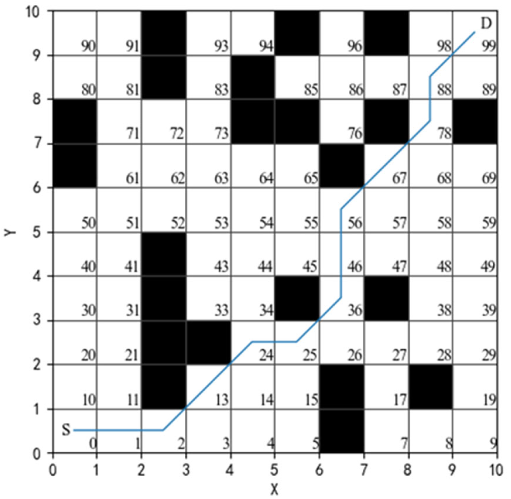
Environment modeling is very important for path planning systems, affecting the length of the search path and the search time. Firstly, we need to capture the environment information, including static information and dynamic information, and then build the environment model for the obtained environment information, which represents the real environment of the mobile robot during the driving process. Since grid maps are simple, effective, and easy to implement, the grid method is used to model the environment of the mobile robot’s operating space, and the size and number of grids are determined by comparing the size of obstacles and the robot’s operating space. As shown in
Figure 1, the white grid indicates the area through which the robot can pass, the black grid indicates the location of obstacles in the operating environment, (0,0) is the starting point location, and (10,10) is the target point location. Numbers are assigned to the grids in a raster map, mainly for ease of coding solutions in post-sequence algorithm programs and for easy representation of the final solution path. A global static path that is finally planned can be represented by a series of numbers in the grid. To facilitate the experiments, it is assumed that the boundaries of both the map and the obstacles are established considering the safe distance of the robot, so that the robot can be considered as a prime point in the grid map.
When searching for a path, the grid position needs to be marked; there are two main ways of marking: one is the coordinate method and the other is the sequence method.
- (1)
Coordinate method: the two mutually perpendicular sides of the grid map are used as the X and Y axes of the plane rectangular coordinate system and any position in the grid map can be represented by coordinates.
- (2)
Sequential method: each grid is incrementally marked according to certain horizontal and vertical rules and each grid is numbered accordingly.
The formula for converting the above two methods is as follows:
In Equation (1),
,
is the coordinate of the grid map obtained by the coordinate method;
denotes the grid number obtained by the sequence method;
is the grid scale size;
denotes the remainder function;
denotes the division function and rounds down. Taking
Figure 1 as an example, the obtained feasible paths are marked with blue lines and the feasible paths obtained using the above two methods are expressed as:
When we design the path planning algorithm, we use the sequence method to represent the feasible path of the mobile robot for the convenience of the representation and we also combine the conversion of coordinate method and the sequence method in the process of algorithm solving and code development with Equation (1).
3.2. Build the Fitness Function
In order to avoid the path optimization of the dynamic window approach to local optimum, we firstly use the genetic algorithm to plan a static global path, so that the dynamic path planned by the robot during the driving process is always close to the global optimum path. During the movement of the robot, the shorter the movement distance, the lower the energy consumption and, the smoother the turning transition, the higher the safety. Therefore, in this paper, the motion distance from the robot’s starting position to the target position (energy consumption), the sum of the turning angles, and the number of turning points during the robot’s motion (safety) are used as the objective function of the multi-objective optimization problem, the robot’s motion coordinate position is used as the decision variable, and the physical boundary and obstacle coordinates of the constructed map are used as the constraints. The following mathematical model was developed for the fitness function as shown below.
In the above Equation (2), denotes the points on the path, denotes the length of the path, denotes the sum of the angles on the path, denotes the number of turning points on the path, , , denotes the weight coefficients, and denotes the target value of the fitness function. Equation (3) indicates that the path formed does not cross the obstacle and does not exceed the boundary of the travelable area.
For the above objective function and constraints, it is obvious that they belong to the multi-objective multi-constraint nonlinear model and it is difficult to solve its exact solution. When the traditional genetic algorithm is used to solve the problem, the search efficiency is low and it is easy to fall into the local optimal solution, so this paper uses the improved genetic algorithm to solve the problem.
4. Improved Genetic Algorithm
4.1. Population Initialization
Traditional genetic algorithms (TGA) [
19,
20,
30] have the disadvantage of great randomness in initialization, which cannot guarantee the diversity of population individuals and can easily fall into local optimal solutions. In the initialization of the population, we determine whether the population satisfies the diversity by calculating the variance of the fitness of all individuals in the population; the diversity requirement is satisfied when the variance of the fitness of individuals in the population is greater than the threshold
; otherwise, a new population of individuals is generated. The specific population initialization is described as follows.
First, the population is initialized by dividing the population into two parts, A and B. The population size of each part is , population A is initialized by random generation, and population B is initialized by the variance threshold discriminant method. Specifically, represents the fitness of each individual in the population, indicates the mean fitness, and is the variance of the population. The initialized population is qualified when . If the population is not qualified, we need to pick chromosomes randomly and regenerate them until the population variance satisfies . By combining sub-populations A and B into one population for crossover and mutation of the genetic algorithm, we can maintain both the randomness and the diversity of the population with the above method.
4.2. Adaptive Selection, Crossover, Mutation, and Elite Strategy
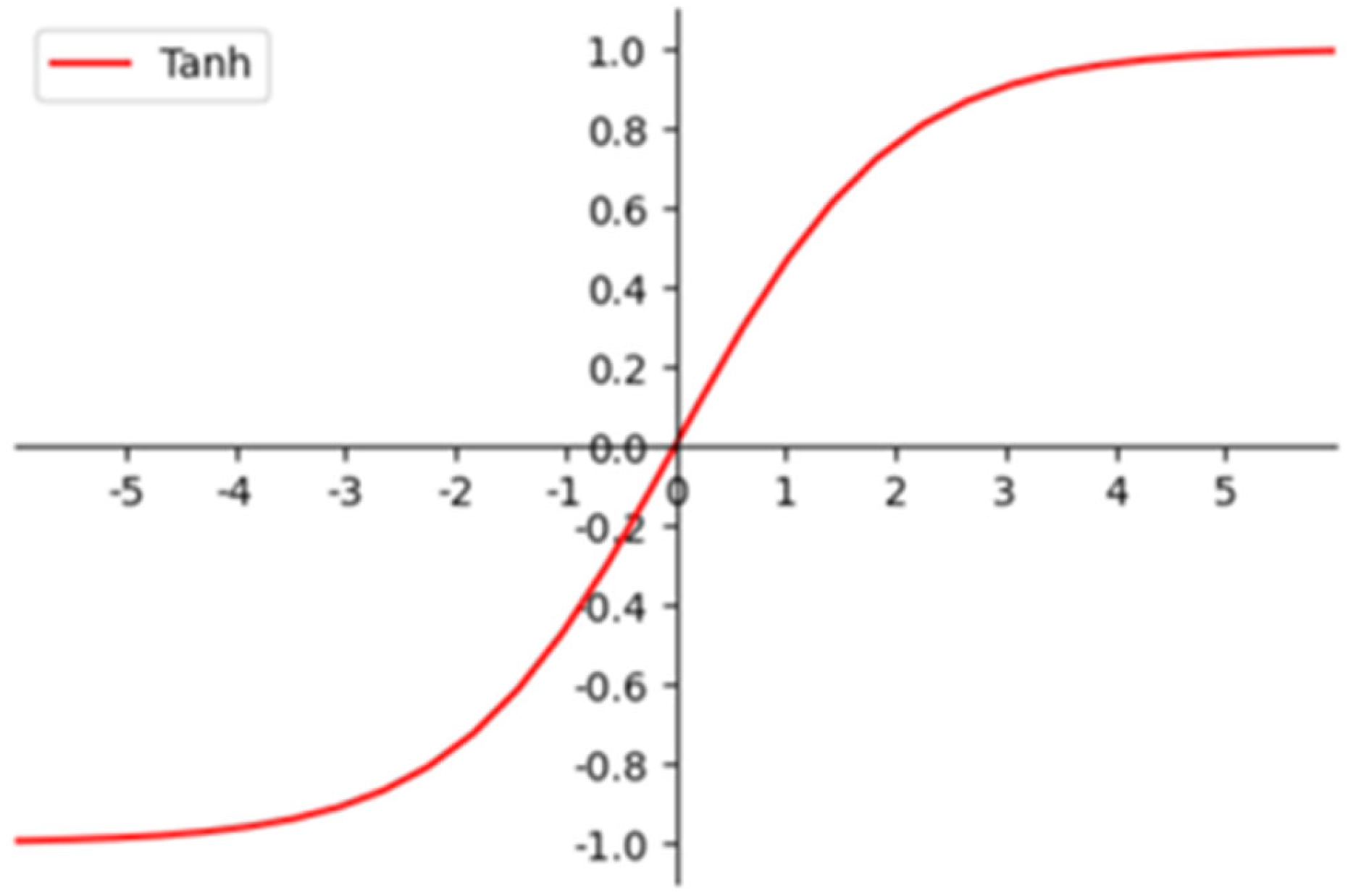
In the iterative process of genetic algorithms, the values of selection probability, crossover probability, and variation probability have a great influence on the efficiency of generating new individuals. Traditional genetic algorithms usually use fixed crossover probabilities and genetic probabilities, which can ensure the generation of new individuals but tend to destroy the more adaptive individuals when the population evolves to a certain level. In order to retain elite individuals, promote population iterative diversity, and obtain the global optimal solution early, an activation function
(as shown in
Figure 2) is introduced with adjusted selection probability
, crossover probability
, and variation probability
.
In Equation (4) above,
,
,
,
,
,
represent the maximum and minimum values of the selection probability, the maximum and minimum values of the crossover probability, and the maximum and minimum values of the variance probability, respectively.
represents the fitness of individuals in the generation
population and
represents the average fitness of the generation
population.
In order to prevent the loss of superior genes during crossover and mutation of the population, we adopt the elite individual genetic retention strategy. At each population iteration, optimal individuals are selected without crossover and mutation and directly enter the next iteration. is calculated according to Equation (5), where is the elite retention factor,
represents the number of current iterations, and represents the number of final iterations. When the population starts to iterate, the elite retention factor is set larger in order to retain the best individuals and to speed up the search for the optimal solution. When it proceeds to the late iteration, the elite retention factor is gradually reduced in order to avoid the population from falling into local optimal solutions and to increase the diversity of population iteration.
4.3. Regeneration Operator
In the iterative process of the genetic algorithm, due to the particularity of path planning, when the individuals of the population cross and mutate it is likely that the paths represented by the generated individuals are discontinuous or pass through an obstacle and then the individuals generated by the cross or mutation operation are discarded. In order to keep the population size unchanged, a regeneration operator is added after crossover and mutation operations to generate new individuals to replace unqualified individuals generated during crossover or mutation operations. In order to expand the search range of the optimal solution and to make the regenerated population diverse, new population individuals are generated in the following way during the population initialization.
We use to denote the population size and to denote each individual of the population, where represents the chromosome of each individual and represents the chromosome of the optimal individual. When generating new population individuals, the similarity between chromosomes and is calculated for each resulting chromosome (this can be performed using Euclidean distance). Finally, the average population similarity . When , the generated population satisfies the diversity principle of the initialized population. Otherwise, chromosomes are randomly selected and regenerated until the initialized population is .
4.4. Key Point Extraction Strategy
Although the global optimal path planned by the above improved genetic algorithm has been optimized for smoothness to some extent, there are still some redundant points and unnecessary turning points that are not completely eliminated, which is not conducive to the control of the robot. To address this problem, we propose a key point or node extraction strategy with reference to Fazle et al.’s study [
31,
32,
33,
34]; the specific implementation steps are described below.
Extract the global path turning point using the three-point one-line method. Starting from the second node on the global path, if the current node is on the same line with the previous node and the next node, the current node is a redundant point, delete the redundant point and update the path. Iterate through all path nodes in turn, delete redundant points, and finally obtain the path sequence containing only the starting point, turning point, and end point.
Extract the key points. Let the sequence of global path turning points be
after removing redundant points. Make a straight line from
, connect
in turn, determine whether the straight line
passes through the obstacle, if so, then the node
is a necessary node of the path and must be a key turning point, add node
to the set
containing key nodes. Otherwise, node
is determined to be a redundant node and the nodes in node set
are connected backward from
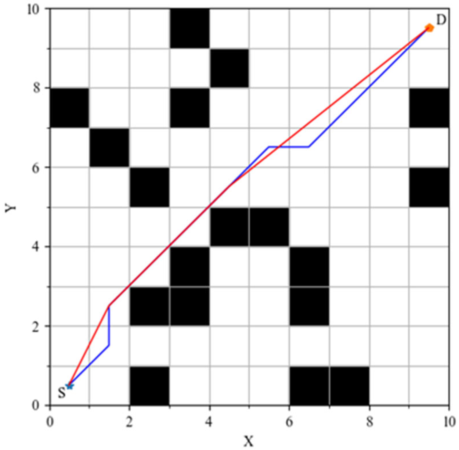
until the end of the global path is connected. Finally, the set of all key nodes
is obtained, as shown in
Figure 3. The blue curve represents the path planned by the traditional genetic algorithm and the red curve represents the path planned after the key points are extracted.
4.5. Improved Genetic Algorithm Process
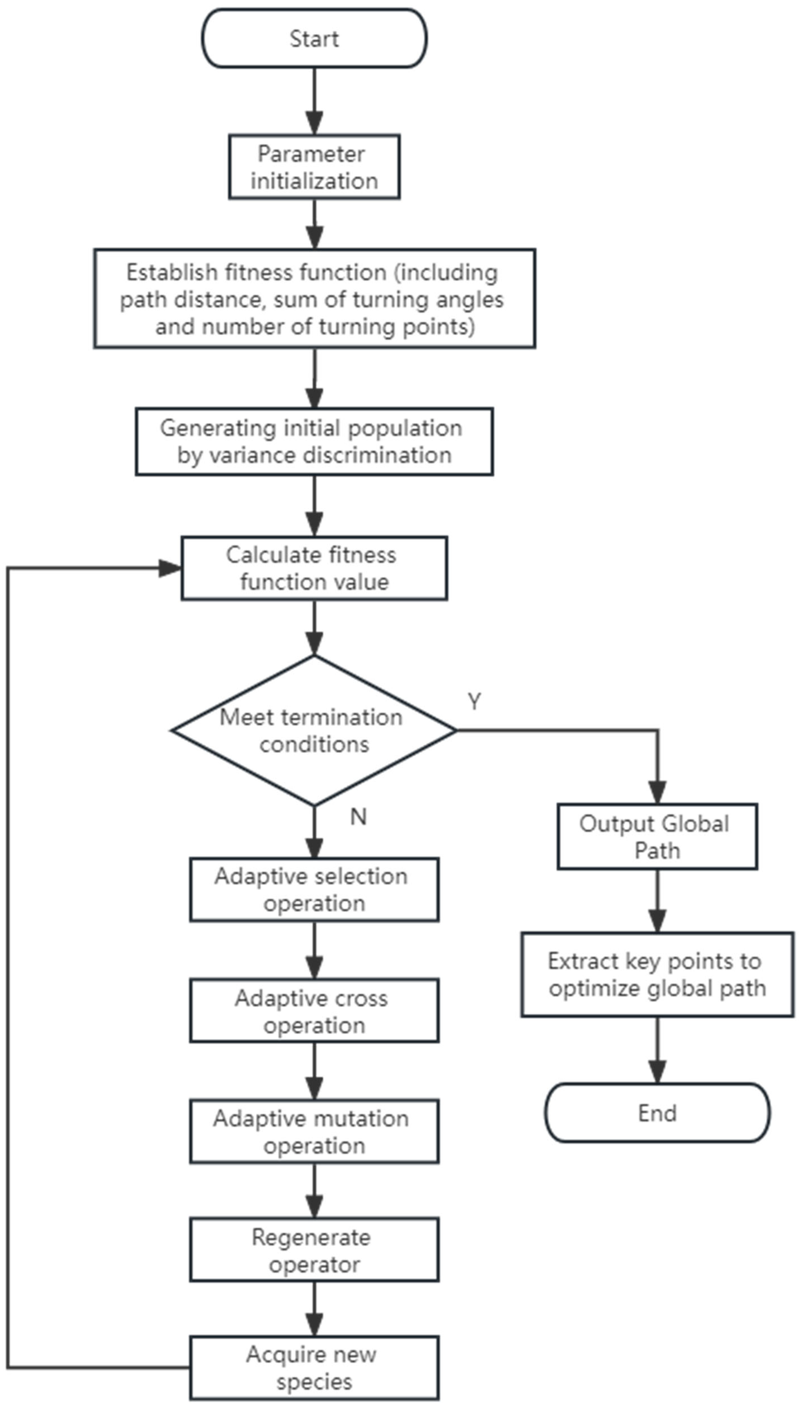
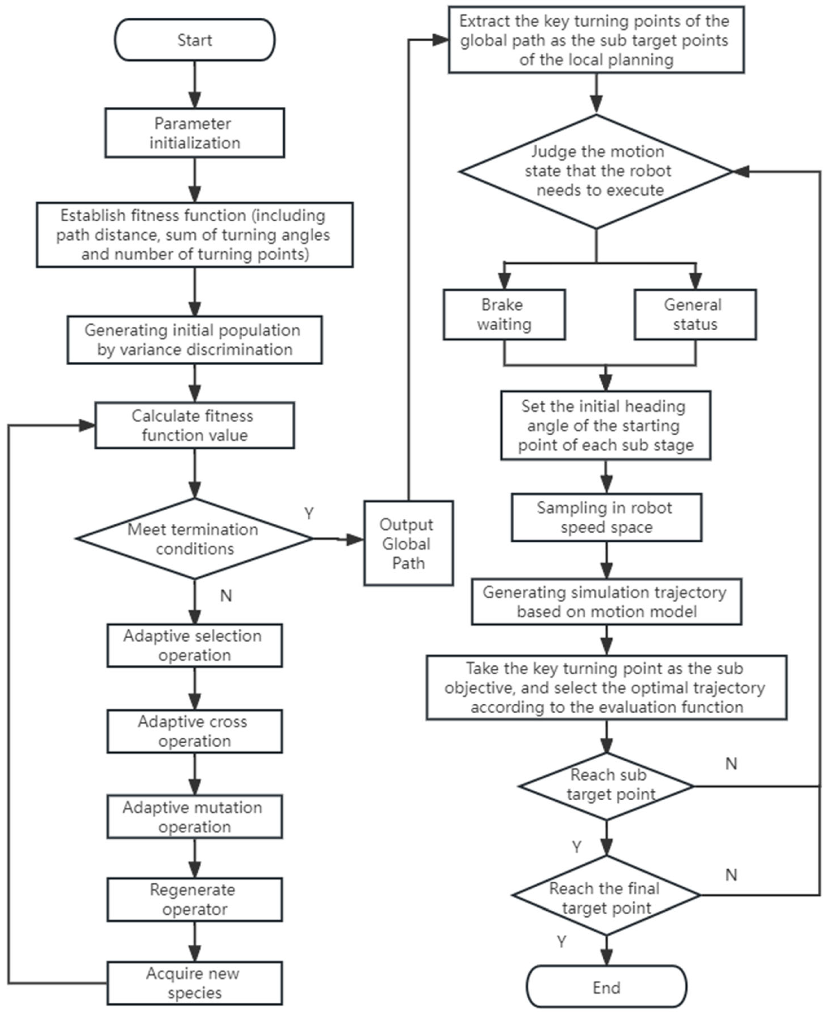
The flow chart of the improved genetic algorithm (IGA) proposed in this paper is shown in
Figure 4. The termination condition of the algorithm is that the optimal solution does not change in 50 consecutive iterations of evolution or the number of evolutions reaches the upper limit of the system preset.
5. Fusion of Improved Genetic Algorithm and Dynamic Windowing Algorithm
5.1. Robot Motion Model
Since the paths derived from the genetic algorithm are static, in complex scenarios the mobile robot is prone to encounter moving objects when driving. To make the path planning problem dynamic, we use the dynamic window approach for local path planning.
The dynamic window approach spatially samples the velocity of the mobile robot in the window region and simulates the motion trajectory of the robot. The motion state of the robot is fed by its linear and angular velocities,
represents the trajectory, the best trajectory is selected among all feasible trajectories by the evaluation function. During the time interval
, the robot is assumed to move in a uniform linear motion with the following kinematic model:
In Equation (6), and represent the coordinate positions of the mobile robot at time , respectively; is the heading angle of the mobile robot at time ; is the linear velocity of the mobile robot; represents the angular velocity of the mobile robot.
In the velocity search space, the range of sampled velocities is constrained according to a certain range of infinitely many groups
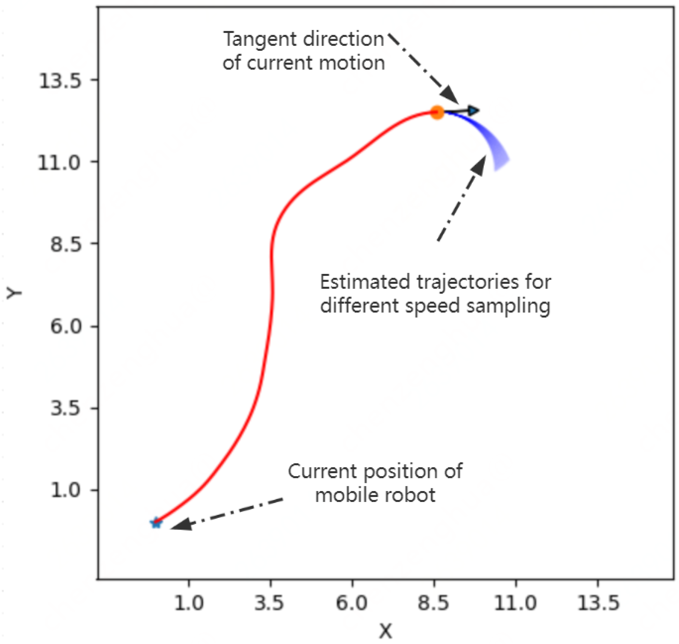
obtained from the mobile robot and its environment. The constraints can be divided into three types: the robot body velocity constraint, the motor acceleration constraint, and the obstacle distance constraint. The velocity sampling results in the simulation experiments are shown in
Figure 5.
Mobile robot body speed constraint:
Mobile robot motor acceleration constraint (the upper and lower limits of the robot speed are caused by the mobile robot acceleration being limited by the motor performance during the sampling period under the dynamic window):
In Equation (8), and represent the linear and angular velocities of the robot at the current moment, respectively; and represent the minimum and maximum acceleration of the linear velocity, respectively; and represent the minimum and maximum acceleration of the angular velocity, respectively.
Obstacle distance constraint. Considering the safety of the robot when moving, it is necessary to ensure that the robot does not collide with obstacles, then the velocity space constraint of the robot is represented, as shown in Equation (8), under the maximum deceleration condition during local dynamic path planning.
In Equation (9), is the nearest distance from the obstacle on the trajectory corresponding to velocity space .
5.2. Evaluation Function
The evaluation function of the mobile robot was constructed, as shown in Equation (10), as the indicators of the robot’s moving speed, traveling distance, obstacle avoidance ability, and path azimuth are crucial to the efficiency of the robot. The optimal simulated trajectory is selected according to the evaluation function
and the mobile robot is driven by the corresponding
for path planning.
In Equation (10), represents the angle between the line connecting the end of the simulated trajectory to the target position and the current robot heading under the current given speed pair
; represents the distance between the end of the simulated trajectory and the target position under the current given speed pair
; indicates the minimum distance from the end of the simulated trajectory to the obstacle under the current given speed pair ; is an evaluation sub-function for the current given speed pair . In above Equation (10), is a new sub-function added in the traditional dynamic window approach in this paper, which can make the simulation track finally selected by the algorithm closer to global optimization. and are the weight coefficients of each evaluation sub-function.
5.3. Selection of the Node Heading Angle
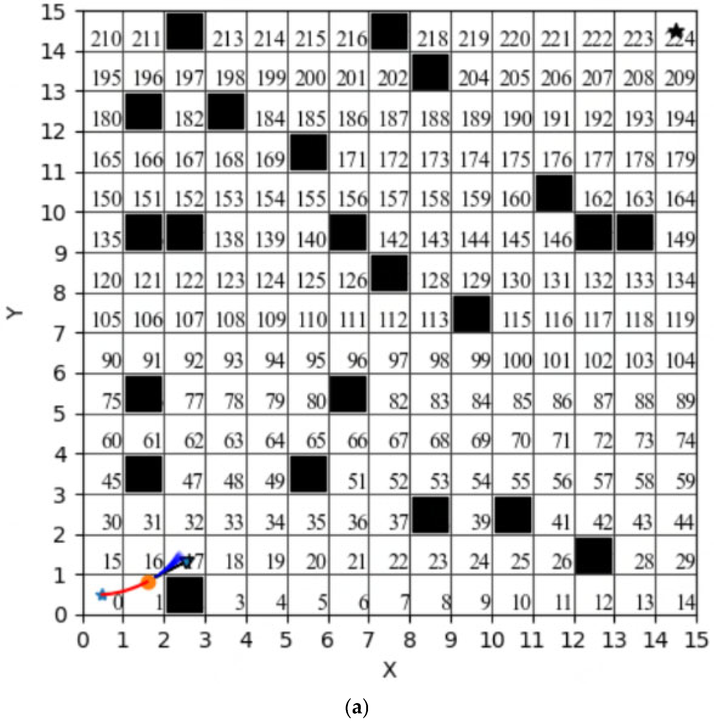
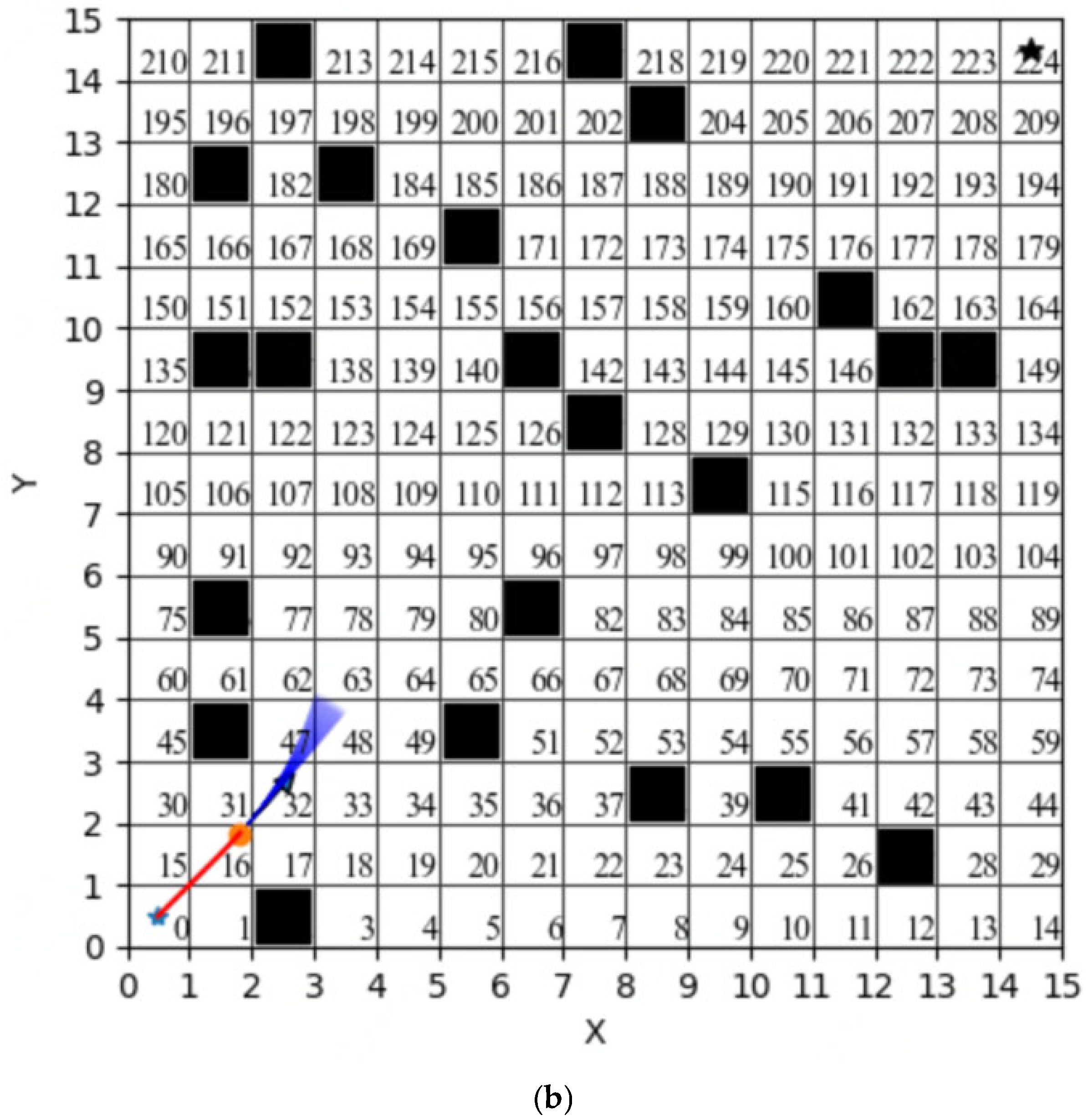
In the traditional dynamic window approach (traditional DWA), the initial heading angle of the mobile robot is randomly given or is a fixed angle based on empirical convention. When the angle deviation from the target point is large, the initial search route detour will occur, increasing the redundancy of the robot operation path, as shown in
Figure 6. In addition, since this paper integrates the dynamic window approach with the global path planned by the improved genetic algorithm (IGA), the dynamic window approach in this paper will be divided into several stages for local path planning and the path nodes on each stage are the key turning points on the global path planning of the improved genetic algorithm. Therefore, this paper proposes to dynamically set the initial heading angle of the mobile robot by the angle between the line that connects the starting point with the first sub-target point and the horizontal direction. The initial heading angle for the local path planning of the next path stage inherits the heading angle at the end of the previous stage to ensure the smoothness of the generated path. We set the coordinates of the starting point (the blue five-pointed star in the figure) as
and the coordinates of the first sub-target point as
. The initial heading angle of the mobile robot (
) can be calculated by Equation (11).
5.4. Adaptive Adjustment of Robot Motion State
In the traditional dynamic windowing approach, the robot has a single state of motion and can only move towards the target point and continuously avoid obstacles and it will keep moving continuously as long as it does not reach the target point. In some scenarios, the traditional dynamic window approach may plan a path with a direction of movement similar to that of the moving obstacle or a turn angle that is too large when the moving distance is too long and the path is not optimal or better. Referring to previous studies [
35], we propose to increase the motion state of the target robot braking and waiting when the target robot and the moving obstacles satisfy certain conditions so as to avoid planning unnecessarily long paths and to realize the obstacle avoidance function. When the robot selects the brake-and-wait operation, the following conditions should be met for moving obstacles: (1) in the direction of the target robot forward(the red arrow in the figure); (2) with the robot distance less than
; (3) moving speed greater than
(obstacle moving speed can be detected by the sensor installed on the mobile robot); (4) the angle between obstacle moving direction and the robot’s current planning heading (
) should meet
, as shown in
Figure 7. In this case, the robot performs an emergency brake and waits until the moving obstacle disappears in front of the planned path (when the distance between the robot and the moving obstacle is greater than
) before moving forward. The size of parameters
and
can be set according to the robot’s own situation, where
denotes the distance between the mobile robot and the dynamic obstacle and
denotes the movement speed of the dynamic obstacle.
5.5. Fusion Algorithm
Our improved genetic algorithm has good results in shortening robot paths and reducing robot path nodes, but there are still problems such as large path turning angles and insensitive avoidance of dynamic obstacles. The dynamic window algorithm has an inherent advantage in avoiding moving obstacles, but this algorithm tends to fall into a local optimum and performs poorly in global path planning. In order to plan a smooth robot path that is globally optimal and can avoid obstacles in time, in this paper the two algorithms are effectively fused to retain their respective advantages. We first plan the global path by an improved genetic algorithm to extract the key points of the global path, then use these key points as temporary sub-target points for each stage in the dynamic window approach to reduce the impact of moving obstacles on the overall path of the robot. At the same time, the global dynamic path planned by the dynamic window approach is closer to the global static path planned by the improved genetic algorithm in this paper. The flow of the fusion algorithm is shown in
Figure 8.
6. Simulation Experiment and Data Analysis
In order to verify the feasibility and effectiveness of the improved genetic algorithm (IGA), this paper uses the 2D grid map method, which is simple to code and easy to implement, to establish a simulation environment for comparison with the traditional genetic algorithm (TGA), where the black grid indicates the obstacles and the white grid indicates the passable path points; the following experiments are designed for verification.
The experimental environment for the algorithm in this paper is a 64-bit WIN10 operating system running with 16 GB of RAM, a CPU of 11th Gen Intel(R) Core(TM) i7-11800H @ 2.30 GHz 2.30 GHz, and the algorithm is programmed in Python language with the execution version of Python 3.9.
6.1. Simulation Experiment and Analysis of Improved Genetic Algorithm
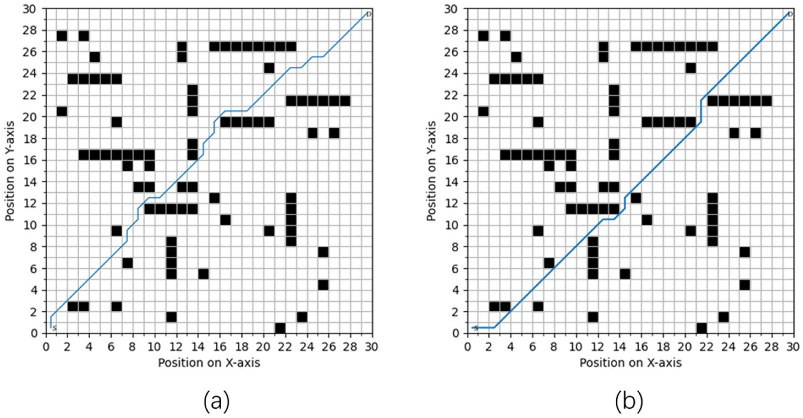
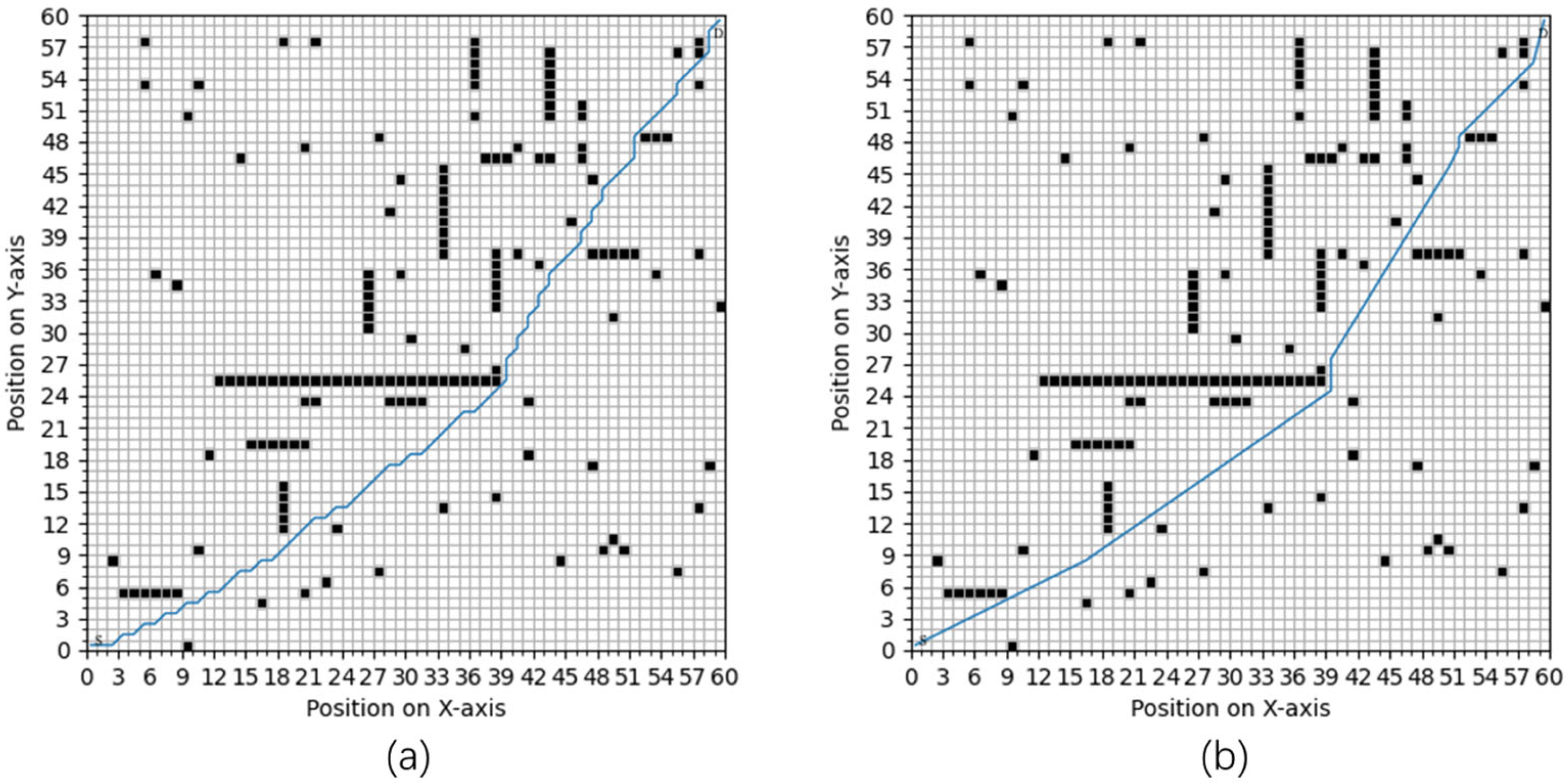
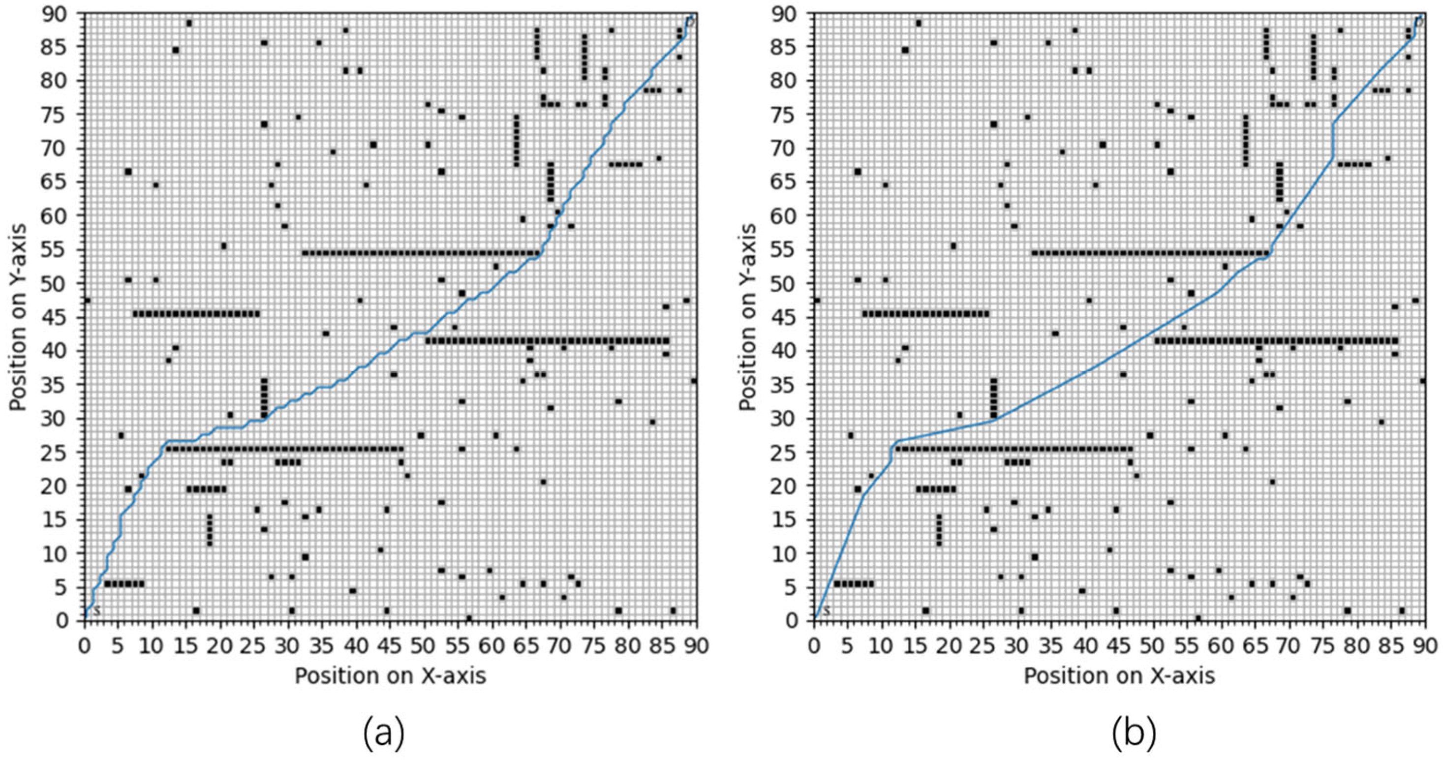
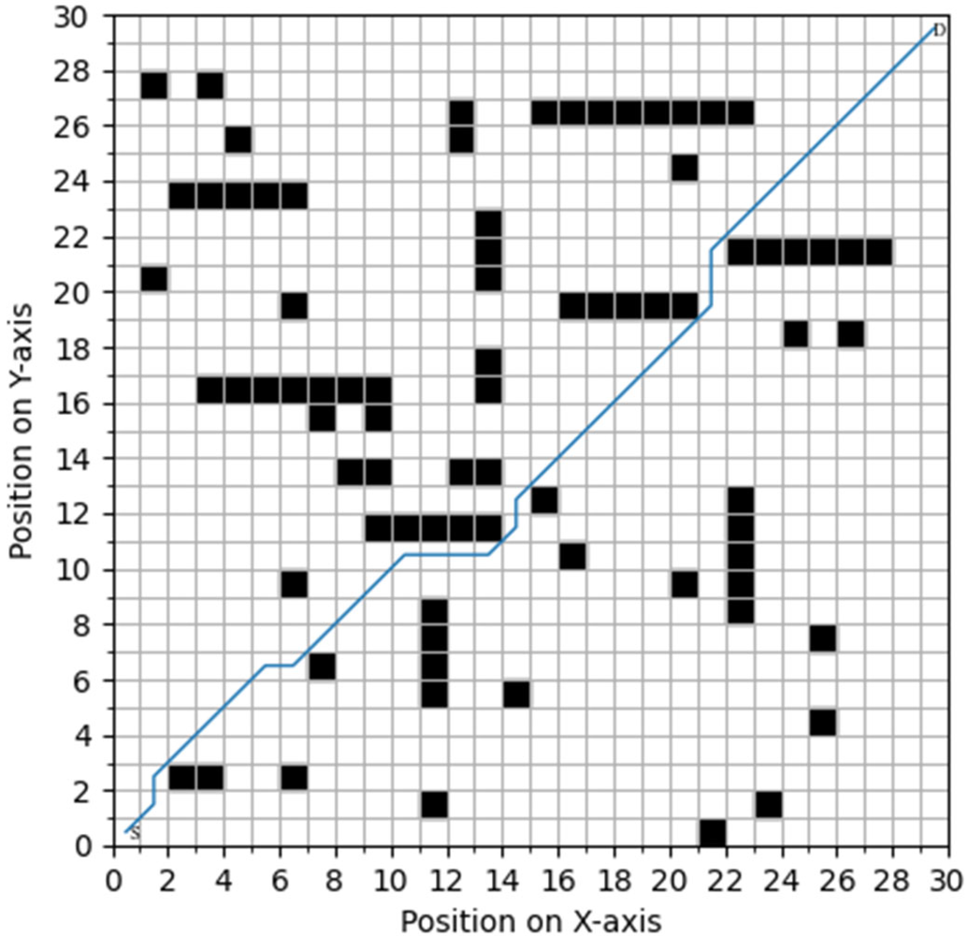
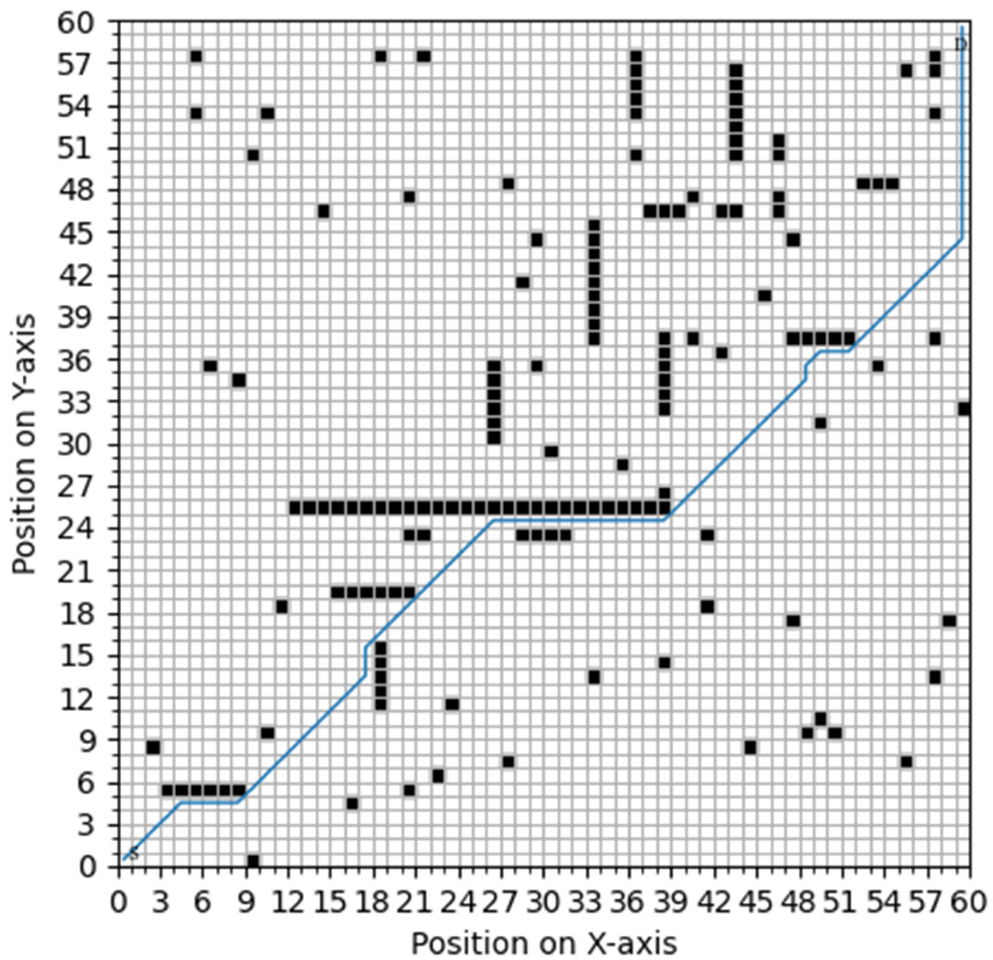
In order to verify the performance improvement of the improved genetic algorithm in terms of planning length of path, running time of program, and number of folding points (key points), simulations were conducted before and after the improvement of the genetic algorithm in grid maps of 30 × 30, 60 × 60, and 90 × 90 sizes; the results are shown in
Figure 9,
Figure 10 and
Figure 11, respectively. The statistics of the above simulation experiments are shown in
Table 1.
Comparing our improved genetic algorithm with the traditional genetic algorithm, three sets of path planning maps are obtained in different sizes of maps (
Figure 9,
Figure 10 and
Figure 11). It can be seen that in the same static environment, compared with the traditional genetic algorithm, the path planned by the improved genetic algorithm eliminates redundant inflection points, resulting in shorter path lengths and improved smoothness. To accurately describe the path optimization mechanism in
Figure 9,
Figure 10 and
Figure 11, we further analyze the path length, algorithm running time, number of key points, and the degree of their improvement produced by the robot paths formed by the conventional genetic algorithm versus those formed by our improved genetic algorithm in raster maps of different sizes. The results (
Table 1) show that: the traditional genetic algorithm converges slowly and is prone to the phenomenon of “early maturity”, which determines more key points, poor path smoothing, and long path length.
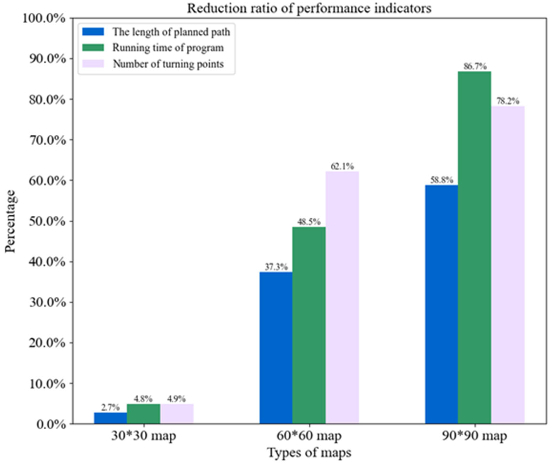
The improved genetic algorithm determines whether the population meets the diversity by calculating the fitness variance of all individuals in the population, which overcomes the prematurity of the traditional genetic algorithm and prevents the algorithm from falling into the local optimal solution prematurely. By improving the adaptive selection, crossover and mutation probability, elite retention strategy, and regeneration operator, the search scope of the optimal solution is expanded and the speed of solving the optimal solution and the quality of the optimal solution are improved. Finally, the number of turning points on the static global optimal path is further reduced through the key point extraction strategy. Through the above simulation experiments in different grid map environments, it can be seen that the improved genetic algorithm proposed in this paper reduces the planned global path by 2.7%, 4.8%, and 4.9% respectively, reduces the running time of the program by 37.3%, 48.5%, and 62.1% respectively, and reduces the number of key points on the global path by 58.8%, 86.7%, and 78.2%, respectively. To further show the degree of improvement, we have plotted
Figure 12, where green represents the traditional genetic algorithm and blue represents our improved genetic algorithm. It can be seen that our improved genetic algorithm has significant advantages in terms of running time and the number of turning points and the path length is also somewhat reduced.
In
Figure 13 and
Figure 14, the iterative plots of the fitness of the two different genetic algorithms show that the traditional genetic algorithm (TGA) converges to a state of convergence only at about 120 generations of iteration for three different types of maps, while our proposed improved genetic algorithm (IGA) converges to a state of convergence at the 80th generation of iteration for three different types of maps and is able to obtain lower fitness values. This means that the improved genetic algorithm proposed in this paper can converge faster than the traditional genetic algorithm and can obtain a better global optimal solution. From the iterative plots of population fitness standard deviation in
Figure 14, it can be seen that the variance of population fitness of the improved genetic algorithm proposed in this paper has been larger than that of the traditional genetic algorithm and the variance of population fitness of the improved genetic algorithm fluctuates more, which indicates that the population diversity of the improved genetic algorithm has been better than that of the traditional genetic algorithm in the process of genetic iteration and thus is more conducive to the rapid population, achieves the global optimal solution, and avoids becoming trapped in the local optimal solution. Finally, it can be seen jointly in
Figure 15 and
Table 1 that when the map size is increased from 60*60 to 90*90, the optimization effect of each performance index such as path length, program running time, and number of path turning points is more obvious in the improved genetic algorithm; especially, the percentage of program running time reduction increases from 48.5% to 62.1%.
6.2. Simulation Experiments and Analysis of Fusing Improved Genetic Algorithm and Dynamic Window Approach
In order to verify the feasibility and effectiveness of a path planning algorithm that combines improved the genetic algorithm and the dynamic window approach proposed in this paper, simulation experiments comparing the traditional dynamic window approach and the fusion algorithm of this paper are carried out by programming in Python under different simulation environments in this paper.
This experiment compares the traditional dynamic window approach and the fusion algorithm proposed in this paper in a simulation experiment under the 11*11 map environment in 5.1. The starting point of the map (the five-pointed star in the figure) is (0,0) (the grid numbered 0 in the map) and the ending point (the red point in the figure) is (9,9) (the grid numbered 108 in the map). The red line represents the track of the robot’s movement. As shown in
Figure 16, we find that, compared with the fusion algorithm, the path obtained by the traditional dynamic window approach falls into local optimum and does not obtain the optimal path, which has redundant sections, although the path is smooth. The fusion algorithm can achieve better smoothness and a shorter path and the path length is shortened from 14.562 to 12.744. Our improved fusion algorithm first uses an improved genetic algorithm to obtain a static global optimal path and then uses the key turning points on the static global optimal path as subgoals of multiple stages of the improved dynamic window approach in this paper to plan a global dynamic path. The method improves the problems of poor smoothness and real-time performance of the static global path planning algorithm and improves the defect that the local path planning algorithm is prone to fall into local optimal solutions due to the combination of key turning points of the global path and the generated path is more consistent with the kinematic model of the robot.
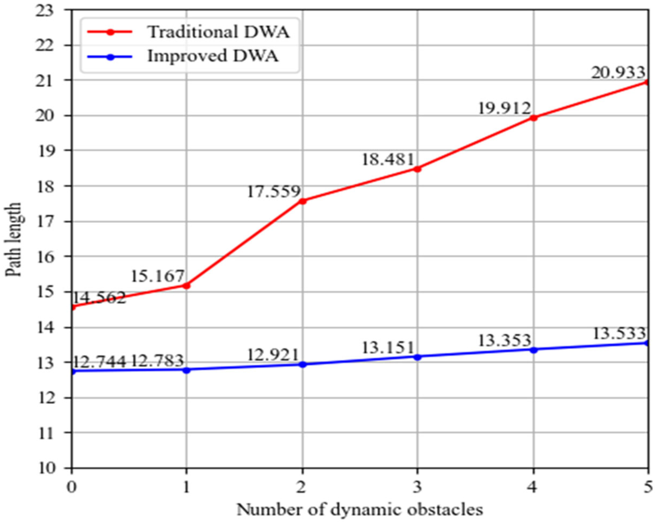
To verify the feasibility of the improved fusion algorithm, Experiment II is further conducted in the grid map environment of Experiment 1. We observe the path planning capability of the traditional dynamic window approach and the improved fusion algorithm of this paper by gradually increasing the number of dynamic obstacles. As shown in
Figure 17, the path length increases gradually with the number of dynamic obstacles, but the path lengths generated by the traditional DWA are all larger than the improved fusion algorithm in this paper. The improved fusion algorithm generates path lengths that grow slowly and are more stable as the number of obstacles increases from two to five.
Next, we show the path tracks of the robot when it encounters dynamic obstacles by adding dynamic obstacles to the grid map. We set the black grid for static obstacles and the blue grid for dynamic obstacles in
Figure 18 and
Figure 19. The starting point (the five-pointed star in the figure) of the map is (0,0), the subfigure(a), (b) (c), (d) in the
Figure 18 and
Figure 19 represent the dynamic movement engineering of the mobile robot. Among them,
Figure 18 shows that, in the traditional dynamic window approach, when the robot encounters a dynamic obstacle it will perform an obstacle avoidance operation by going around, thus causing the planned path to become longer.
Figure 19 shows the path planned by the fusion algorithm proposed in this paper. When a dynamic obstacle meeting the conditions described above is encountered, the robot will stop moving forward, will wait for the current dynamic obstacle to move away, and then will follow the planned path, thus greatly reducing the length of the planned path. Through the above experiments, it can be seen that the fusion algorithm proposed in this paper can enable the mobile robot to perform effective obstacle avoidance and be able to find the optimal path.
6.3. Comparison Simulation Experiments and Analysis of Improved Genetic Algorithm and A* Algorithm
In order to verify the performance improvement of our proposed improved genetic algorithm on the planning path length, program running time, and the number of turning points, the improved genetic algorithm and the traditional A* algorithm were simulated and compared in 30*30, 60*60, and 90*90 size raster maps. The mobile robot paths under the two algorithms are shown in
Figure 20,
Figure 21 and
Figure 22, respectively; the algorithm performance improvement metrics are summarized in
Table 2. In addition, we used the diagonal distance as the heuristic function of the A* algorithm. The formula for calculating the diagonal distance is:
In Equation (12), represents the coordinates of two points.
Figure 20,
Figure 21 and
Figure 22 visualize the robot paths planned by A* and the improved genetic algorithm for different sizes of raster maps. The paths planned by the improved genetic algorithm clearly eliminate the redundant internal inflection points, resulting in shorter path lengths and improved smoothness. We analyze the path properties by
Table 2. When the map size is increased from 30*30 to 90*90, the improved genetic algorithm reduces the path length by 1.4%, 7.2%, and 8.6%, the running time by 38.9%, 68.1%, and 69.4%, and the number of key points by 30.0%, 45.5%, and 22.7%. It can be seen that the improved genetic algorithm has obvious advantages over the A* algorithm and the overall performance advantage of the improved genetic algorithm is more obvious as the map size increases, only that the number of key point advantages decreases slightly as the map size increases. In addition, analyzing the operation mechanism of the two algorithms, we find that the genetic algorithm can add more optimization indicators through the fitness function to achieve the overall goal of optimality, while the A* algorithm can only do simple path planning, so the use scenario of the improved genetic algorithm is more diversified.
6.4. Experimental Validation Based on Physical Environment
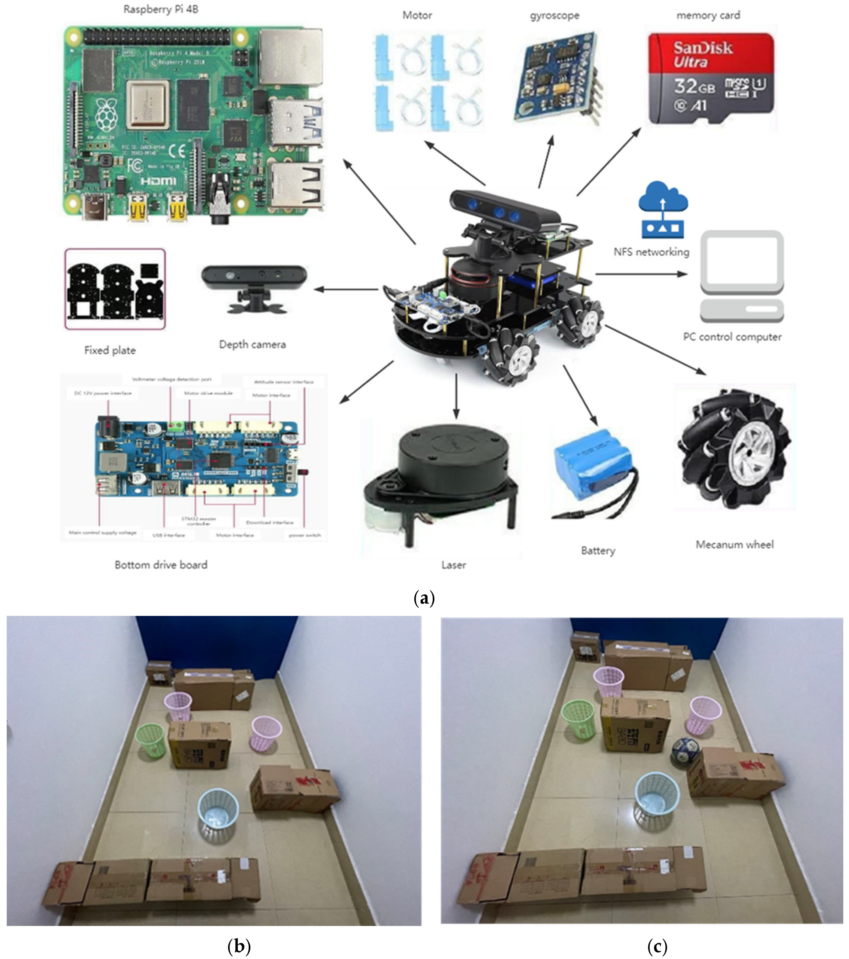
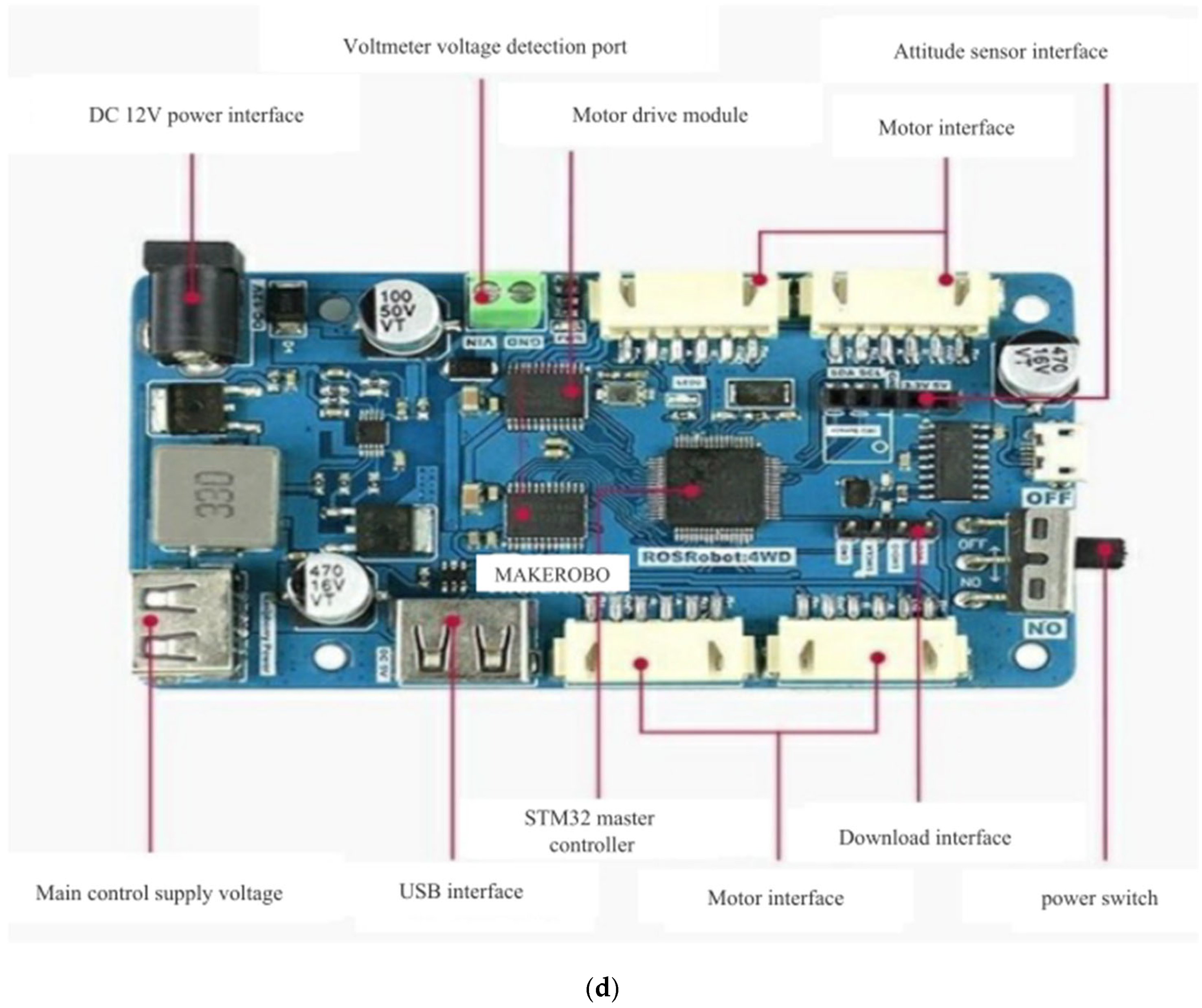
In order to verify the applicability of the fused path planning algorithm based on the improved genetic algorithm and the dynamic window approach proposed in this paper in real environments as well as environments with dynamic obstacles, we built the mobile robot experimental platform (a) and the experimental environments (b) and (c), (
Figure 23). Our experiment consists of hardware such as raspberry Pi 4B be used for IPC, LIDAR, STM32 bottom driver board, depth camera, and McNamee wheel, etc. It is also equipped with Ubuntu 20.04 system, including ROS (Noetic), and the mobile robot and PC controller are connected by NFS distributed networking for communication. To verify the dynamic obstacle avoidance performance of the fusion algorithm, a dynamic obstacle is placed at a certain moment of the robot motion, as represented by the soccer ball in
Figure 24.
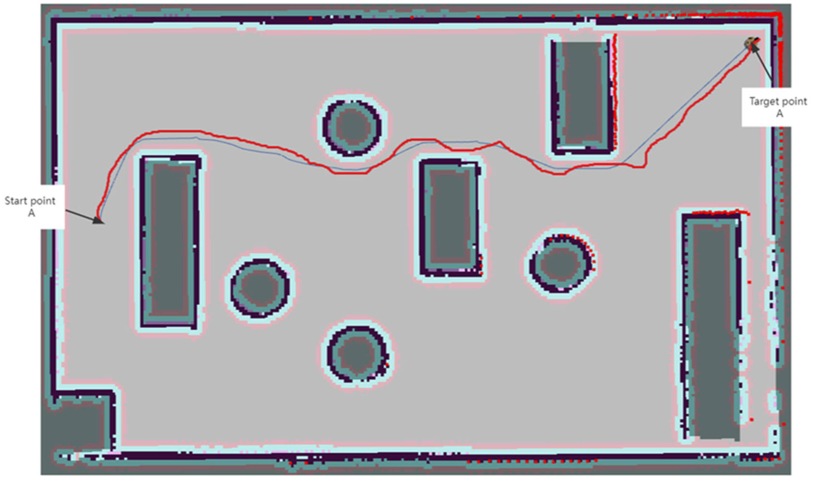
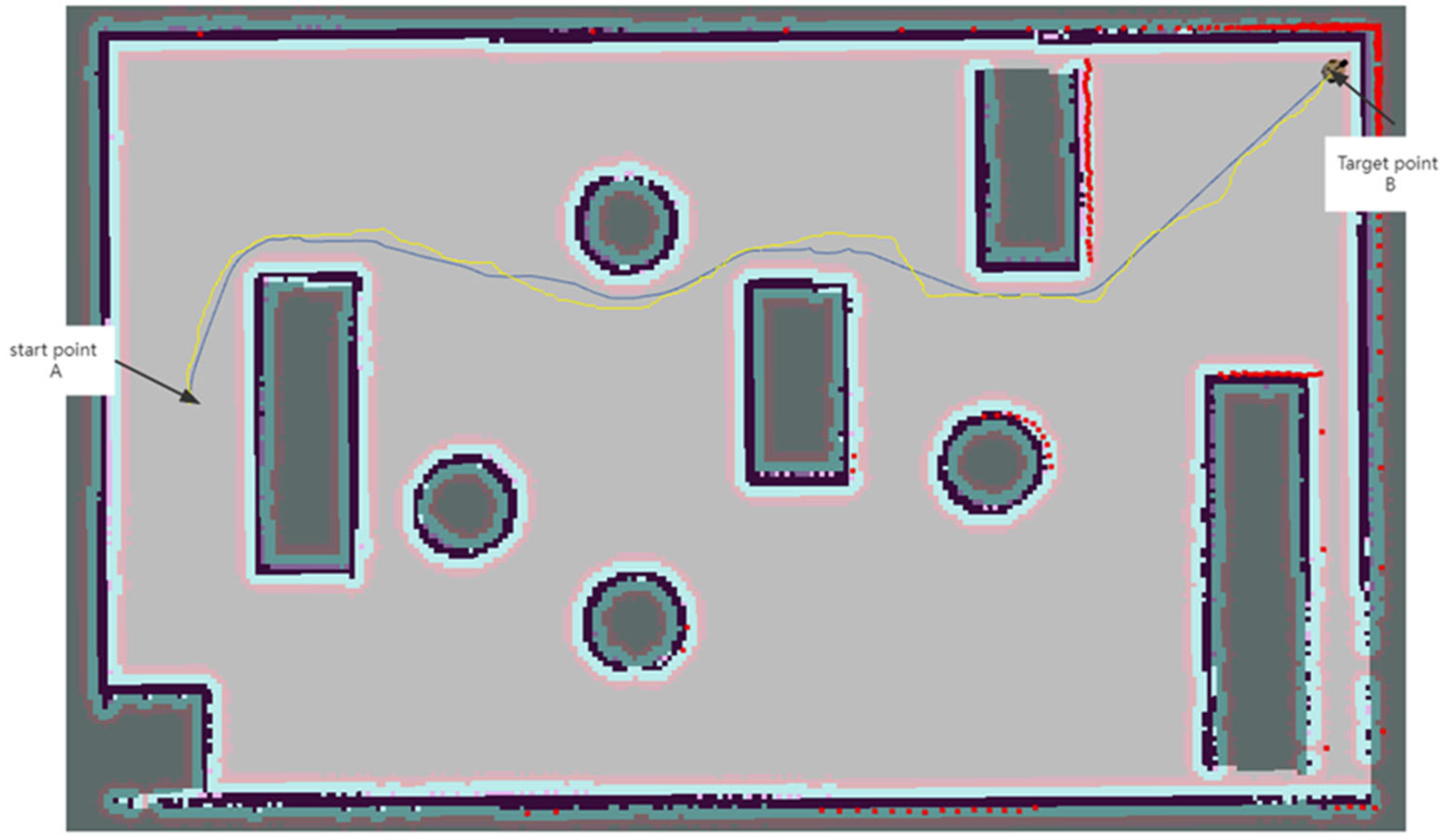
In this paper, we use data from the real environment collected by LiDAR and a depth camera and establish the cost map of the experimental environment by the open-source SLAM algorithm Gmapping.
Figure 24,
Figure 25,
Figure 26 and
Figure 27 show the experimental results observed using Rviz software, where the black area indicates the obstacle, the white around the black area indicates the expansion area, and the gray area indicates the feasible area.
As shown in
Figure 25, the blue trajectory represents the global static path planned by the improved genetic algorithm and the yellow trajectory represents the global static path planned by the traditional genetic algorithm. It is obvious that the global static paths planned by the improved genetic algorithm in this paper are smoother, with fewer path turning points and shorter total path length than those planned by the traditional genetic algorithm.
As shown in
Figure 24, the blue trajectory represents the global static path planned by the improved genetic algorithm proposed in this paper and the red trajectory represents the global static path planned by the traditional A* algorithm. Obviously, the global static paths planned by the improved genetic algorithm proposed in this paper are smoother, with fewer path turning points and shorter total path length than the paths planned by the traditional A* algorithm.
As shown in
Figure 26 and
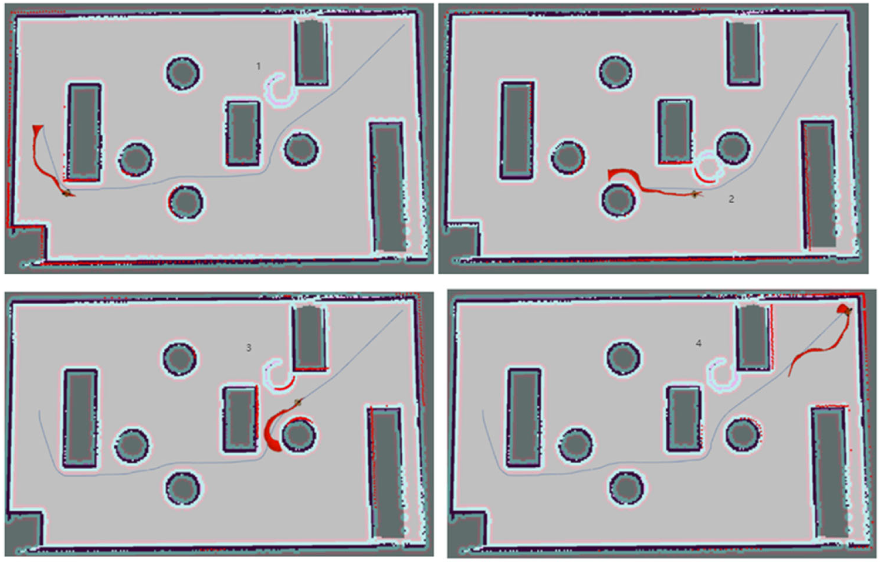
Figure 27, the white hollow circle is a dynamic obstacle that moves randomly. The blue trajectory represents the global static path. The red trajectory represents the local dynamic path of the robot. From
Figure 26, it can be seen that the traditional dynamic window approach generally performs obstacle avoidance operations when encountering dynamic obstacles. This method is more dangerous, because it is easy for the robot to collide with obstacles; with the random movement of dynamic obstacles, the robot planned path is more tortuous and the global optimal path deviation is relatively large. From
Figure 27, it can be seen that the robot using the improved dynamic window approach will take the brake-waiting operation according to the rules proposed in this paper when encountering dynamic obstacles. After the dynamic obstacles leave a certain area, the improved dynamic window approach is used to drive along the global optimal path, which reduces the obstacle avoidance loss of the robot and the possibility of collision with dynamic obstacles and also makes the final driving path of the robot closer to the global optimal.
In summary, it is clear from the comparison of experimental results that the global path planning algorithm used by the traditional genetic algorithm, which only considers the robot’s initial position, target point position, and obstacles in a static map at the start of the robot receiving the driving task, plans paths that are one-time static paths. Our proposed fused path planning algorithm based on the improved genetic algorithm and the dynamic window approach is a local path planning with the turning point on the global path as the stage divider, which can plan the path based on the real-time obstacle position and the path it plans is a real-time dynamic path. Therefore, compared with the simple A* algorithm or the traditional genetic algorithm, the path planned by the fusion algorithm can avoid dynamic obstacles, which is safer, meets the robot’s motion characteristics, and has good real-time performance and at the same time the planned path is shorter compared with the traditional dynamic window approach.
7. Discussion and Conclusions
Aiming at problems including the global static path planning algorithm cannot effectively avoid dynamic obstacles, the local dynamic path planning algorithm lacks global environment information, and the planned paths have poor quality or cannot reach the target point successfully, this paper proposes a dynamic path planning method integrating the improved genetic algorithm and the dynamic window approach.
When the traditional genetic algorithm performs path planning, the algorithm search efficiency is low and it is easy to fall into local optimal solutions. Firstly, we improve the population diversity and speed up the solution of the algorithm by the variance discriminant method during population initialization. To further improve the speed and quality of the solution, we introduce an adaptive elite retention factor as well as improved adaptive selection, crossover, and mutation probabilities to avoid prematurely falling into a local optimum solution. After the crossover and mutation operations, the regeneration operator is added to randomly generate new individuals to avoid population shrinkage in order to improve the population diversity. The traditional genetic algorithm for path planning generally only takes the shortest path as the optimization goal, which results in a low smoothness of the planned path. We add the sum of turning angles and the number of turning points of the planned paths as smoothing indicators to the fitness function and further optimize the paths through the key point extraction strategy to obtain the global optimal paths.
For the traditional dynamic window approach, we improve the robustness of dynamic obstacle avoidance of the robot and reduce path length by improving the simulation trajectory evaluation function, the initial heading angle of each sub-node, the selection of each sub-target node on the global optimal path, and the adaptive adjustment of the robot motion state that is conducive to the obstacle avoidance of the robot. The simulation results in a variety of complex environments show that, compared with the traditional genetic algorithm and the traditional A* algorithm, the improved genetic algorithm in this paper has a higher solving efficiency, smoother global path planning, and a shorter path length. The paths planned by the fusion of the improved genetic algorithm and the dynamic window approach proposed in this paper are smoother. The fusion algorithm can realize real-time dynamic obstacle avoidance and can output control parameters, which is beneficial to the automatic control of the robot and the robustness of dynamic obstacle avoidance. Compared with the traditional dynamic window approach, the fusion algorithm proposed in this paper can ensure the global optimality of the planned paths.
In this paper, we focus on the path planning of single mobile robots in a conventional dynamic environment. In our next work, we will conduct an in-depth study of relevant algorithms for the case of multi-mobile robots and will combine knowledge from the fields of machine vision and reinforcement learning to solve the robot path planning problem in the unstructured environment of smart storage. Meanwhile, the main purpose of this paper is to improve the robot path planning efficiency, reduce the path length, and improve the obstacle avoidance ability of the robot. We will further improve robot path planning algorithms and application scenarios, by studying in a multi-mobile robot scenario how to improve the performance of the path optimization algorithm to make our experiments more practical.
Author Contributions
Conceptualization, J.Z., G.X. and Y.L.; methodology, Z.C. and S.L.; software, Z.C. and G.X.; validation, Y.L. and Z.C.; formal analysis, Y.L.; investigation, Z.C.; resources, Y.L.; data curation, Y.L.; writing—original draft preparation, Z.C. and Y.L.; writing—review and editing, Y.L.; visualization, Z.C.; supervision, J.Z.; project administration, Z.C.; funding acquisition, Y.L. and G.X. All authors have read and agreed to the published version of the manuscript.
Funding
National Key Research and Development Program of China (2018YFB1700602); CAS STS Dongguan Joint Project 20201600200072; National Natural Science Foundation of China under Grants U1909204 & U190920015; CAS Key Technology Talent Program (Zhen Shen); Guangdong Basic and Applied Basic Research Foundation under Grant (2021B1515140034, 2019B1515120030).
Institutional Review Board Statement
Not applicable.
Informed Consent Statement
Not applicable.
Data Availability Statement
The data that support the findings of this study are available from the corresponding author upon reasonable request.
Acknowledgments
This work was supported in part by National Key Research and Development Program of China (2018YFB1700602); CAS STS Dongguan Joint Project 20201600200072; National Natural Science Foundation of China under Grants U1909204 & U190920015; CAS Key Technology Talent Program (Zhen Shen); Guangdong Basic and Applied Basic Research Foundation under Grant (2021B1515140034, 2019B1515120030).
Conflicts of Interest
The authors declare no conflict of interest.
References
- Zeng, Y.; Zhu, L. Research and industrialization of large-scale robot scheduling system under Industry 4.0. China Sci. Technol. Achiev. 2020, 18, 4. [Google Scholar] [CrossRef]
- Sudhakara, P.; Ganapathy, V.; Priyadharshini, B.; Sundaran, K. Obstacle Avoidance and Navigation Planning of a Wheeled Mobile Robot using Amended Artificial Potential Field Method. Procedia Comput. Sci. 2018, 133, 998–1004. [Google Scholar] [CrossRef]
- Chu, K.; Lee, M.; Sunwoo, M. Local path planning for off-road autonomous driving with avoidance of static obstacles. IEEE Trans. Intell. Transp. Syst. 2012, 13, 1599–1616. [Google Scholar] [CrossRef]
- Yazici, A.; Kirlik, G.; Parlaktuna, O.; Sipahioglu, A. A dynamic path planning approach for multirobot sensor-based coverage con-sidering energy constraints. IEEE Trans. Cybern. 2014, 44, 305–314. [Google Scholar] [CrossRef] [PubMed]
- Abdallaoui, S.; Aglzim, E.-H.; Chaibet, A.; Kribèche, A. Thorough Review Analysis of Safe Control of Autonomous Vehicles: Path Planning and Navigation Techniques. Energies 2022, 15, 1358. [Google Scholar] [CrossRef]
- Li, M.; Richards, A.G.; Sooriyabandara, M. Reliability-Aware Multi-UAV Coverage Path Planning Using a Genetic Algorithm; ACM Library: New York, NY, USA, 2021. [Google Scholar]
- Qian, Q.; Wu, J.; Wang, Z. Optimal path planning for two-wheeled self-balancing vehicle pendulum robot based on quantum-behaved particle swarm optimization algorithm. Pers. Ubiquitous Comput. 2019, 23, 393–403. [Google Scholar] [CrossRef]
- Li, S.; Zhang, Y.; Ling, Z.; Zhang, X. Substation Secondary Cable Path Optimization Design Based on 3D Simulation and Improved Dijkstra Algorithm. J. Physics: Conf. Ser. 2021, 2136, 012009. [Google Scholar] [CrossRef]
- Alqahtani, S.M.; Riley, I.; Taylor, S.; Gamble, R.; Mailler, R. MTL Robustness for Path Planning with A*; ACM Library: New York, NY, USA, 2018. [Google Scholar]
- Zhao, H.; Zhou, H.; Yang, G. Research on Global Path Planning of Artificial Intelligence Robot Based on Improved Ant Colony Algorithm. J. Phys. Conf. Ser. 2021, 1744, 022032. [Google Scholar] [CrossRef]
- Koukuntla, S.R.; Bhat, M.; Aggarwal, S.; Jenamani, R.K.; Mukhopadhyay, J. Deep Learning rooted Potential piloted RRT* for expeditious Path Planning. In Proceedings of the 4th International Conference on Artificial Intelligence and Robotics, Guilin, China, 19–21 July 2019. [Google Scholar]
- Sang, H.; You, Y.; Sun, X.; Zhou, Y.; Liu, F. The hybrid path planning algorithm based on improved A* and artificial potential field for unmanned surface vehicle formations. Ocean Eng. 2021, 223, 108709. [Google Scholar] [CrossRef]
- Molaee, T.; Shahrezaee, A. Numerical solution of an inverse source problem for a time-fractional PDE via direct meshless local Petrov–Galerkin method. Eng. Anal. Bound. Elements 2022, 138, 211–218. [Google Scholar] [CrossRef]
- Issofa, N.; Kuetche, C.P.F.; Ateuafack, M.E.; Fai, L.C. Dynamic of the system in a periodic potential, submitted to an electromagnetic wave: Path integral approach. Phys. Scr. 2021, 96, 055702. [Google Scholar] [CrossRef]
- Wang, K.; Li, X.; Gao, L.; Li, P.; Sutherland, J.W. A Discrete Artificial Bee Colony Algorithm for Multiobjective Disassembly Line Balancing of End-of-Life Products. IEEE Trans. Cybern. 2021, 52, 7415–7426. [Google Scholar] [CrossRef]
- Shen, B.Y.; Öztürk, Y.; Wu, W.; Lu, L.; Sheng, J.; Huang, Z.; Zhai, Y.; Yuan, Y.; Wang, W.; Yin, J.; et al. Development of an HTS Magnet for Ultra-Compact MRI System: Optimization Using Genetic Algorithm (GA) Method. IEEE Trans. Appl. Supercond. 2020, 30, 10. [Google Scholar] [CrossRef]
- Ji, K.; Wen, R.; Zong, C.; Ren, Y. Genetic algorithm-based ground motion selection method matching target distribution of generalized conditional intensity measures. Earthq. Eng. Struct. Dyn. 2020, 50, 1497–1516. [Google Scholar] [CrossRef]
- Zhong, Y.K.; Fu, S.M.; Ju, N.P.; Chen, P.Y.; Lin, A. Experimentally-implemented genetic algorithm (Exp-GA): Toward fully optimal photovoltaics. Opt. Express 2015, 23, A1324–A1333. [Google Scholar] [CrossRef]
- Kaur, A.; Kumar, Y. Neighborhood search based improved bat algorithm for data clustering. Appl. Intell. 2022, 52, 10541–10575. [Google Scholar] [CrossRef]
- Cao, L.; Liu, Y. Optimization design and research of simulation system for urban green ecological rainwater by genetic algorithm. J. Supercomput. 2022, 78, 11318–11344. [Google Scholar] [CrossRef]
- Hao, K.; Zhao, J.; Yu, K.; Li, C.; Wang, C. Path Planning of Mobile Robots Based on a Multi-Population Migration Genetic Algorithm. Sensors 2020, 20, 5873. [Google Scholar] [CrossRef]
- Memon, M.A.; Siddique, M.D.; Mekhilef, S.; Mubin, M. Asynchronous Particle Swarm Optimization-Genetic Algorithm (APSO-GA) Based Selective Harmonic Elimination in a Cascaded H-Bridge Multilevel Inverter. IEEE Trans. Ind. Electron. 2021, 69, 1477–1487. [Google Scholar] [CrossRef]
- Sabir, Z.; Raja, M.A.Z.; Alnahdi, A.S.; Jeelani, M.B.; Abdelkawy, M.A. Numerical investigations of the nonlinear smoke model using the Gudermannian neural networks. Math. Biosci. Eng. 2022, 19, 351–370. [Google Scholar] [CrossRef]
- Chang, L.; Shan, L.; Jiang, C.; Dai, Y. Reinforcement based mobile robot path planning with improved dynamic window approach in unknown environment. Auton. Robot. 2020, 45, 51–76. [Google Scholar] [CrossRef]
- Cheng, C.; Hao, X.; Li, J.; Zhang, Z.; Sun, G. Global Dynamic Path Planning Based on Fusion of Improved A* Algorithm and Dynamic Window Approach. J. Xi’an Jiaotong Univ. 2017, 51, 137–143. [Google Scholar] [CrossRef]
- Liu, L.; Yao, J.; He, D.; Chen, J.; Huang, J.; Xu, H.; Wang, B.; Guo, J. Global Dynamic Path Planning Fusion Algorithm Combining Jump-A* Algorithm and Dynamic Window Approach. IEEE Access 2021, 9, 19632–19638. [Google Scholar] [CrossRef]
- Manav, A.C.; Lazoglu, I. A Novel Cascade Path Planning Algorithm for Autonomous Truck-Trailer Parking. IEEE Trans. Intell. Transp. Syst. 2021, 23, 6821–6835. [Google Scholar] [CrossRef]
- Wang, Z.; Liang, Y.; Gong, C.; Zhou, Y.; Zeng, C.; Zhu, S. Improved Dynamic Window Approach for Unmanned Surface Vehicles’ Local Path Planning Considering the Impact of Environmental Factors. Sensors 2022, 22, 5181. [Google Scholar] [CrossRef]
- Lu, L.; Liu, C. Research on Instrument Approach Segment Path Planning under Thunderstorm Weather. Adv. Aeronaut. Sci. Eng. 2022, 13, 150–158. [Google Scholar]
- Elshani, L.; Nui, K.P. Constructing a personalized learning path using genetic algorithms approach. arXiv 2021, arXiv:2104.11276. [Google Scholar]
- Tanjil, F.; Ross, B.J. Deep Learning Concepts for Evolutionary Art. Computational Intelligence in Music, Sound, Art and Design. In Proceedings of the 8th International Conference, EvoMUSART 2019, Held as Part of EvoStar 2019, Leipzig, Germany, 24–26 April 2019; Lecture Notes in Computer Science (LNCS 11453). pp. 1–17. [Google Scholar] [CrossRef]
- Lee, H.V.; Hamid, S.B.A.; Zain, S.K. Conversion of Lignocellulosic Biomass to Nanocellulose: Structure and Chemical Process. Sci. World J. 2014, 2014, 1–20. [Google Scholar] [CrossRef]
- Ma, C.; Zhu, H. Feature selection method applicated PGA. Comput. Eng. Appl. 2009, 45, 107–110, 217. [Google Scholar] [CrossRef]
- Qiao, M.; Liu, C.; Li, Z.; Zhou, J.; Xiao, Q.; Zhou, S.; Chang, C.; Gu, Y.; Guo, Y.; Wang, Y. Breast Tumor Classification Based on MRI-US Images by Disentangling Modality Features. IEEE J. Biomed. Health Informatics 2022, 26, 3059–3067. [Google Scholar] [CrossRef]
- Song, S.; Wu, J. Motion State Estimation of Target Vehicle under Unknown Time-Varying Noises Based on Improved Square-Root Cubature Kalman Filter. Sensors 2020, 20, 2620. [Google Scholar] [CrossRef]
Figure 1.
Simulated grid map.
Figure 1.
Simulated grid map.
Figure 2.
activation function.
Figure 2.
activation function.
Figure 3.
Schematic diagram of extracting key points.
Figure 3.
Schematic diagram of extracting key points.
Figure 4.
Flow chart of improved genetic algorithm.
Figure 4.
Flow chart of improved genetic algorithm.
Figure 5.
Schematic diagram of speed sampling space.
Figure 5.
Schematic diagram of speed sampling space.
Figure 6.
Effect of initial heading angle. (a) Unmodified initial heading angle. (b) Improved initial heading angle.
Figure 6.
Effect of initial heading angle. (a) Unmodified initial heading angle. (b) Improved initial heading angle.
Figure 7.
Schematic diagram of robot braking and waiting.
Figure 7.
Schematic diagram of robot braking and waiting.
Figure 8.
Flowchart of path planning by fusing genetic algorithm and dynamic window approach.
Figure 8.
Flowchart of path planning by fusing genetic algorithm and dynamic window approach.
Figure 9.
Simulation results in 30 × 30 grid map scenario. (a) Traditional genetic algorithm. (b) Improved genetic algorithm.
Figure 9.
Simulation results in 30 × 30 grid map scenario. (a) Traditional genetic algorithm. (b) Improved genetic algorithm.
Figure 10.
Simulation results in 60 × 60 grid map scenario. (a) Traditional genetic algorithm. (b) Improved genetic algorithm.
Figure 10.
Simulation results in 60 × 60 grid map scenario. (a) Traditional genetic algorithm. (b) Improved genetic algorithm.
Figure 11.
Simulation results in 90 × 90 grid map scenario. (a) Traditional genetic algorithm. (b) Improved genetic algorithm.
Figure 11.
Simulation results in 90 × 90 grid map scenario. (a) Traditional genetic algorithm. (b) Improved genetic algorithm.
Figure 12.
Comparison of each performance index before and after algorithm improvement. (a) Path length. (b) Running time. (c) Turning points.
Figure 12.
Comparison of each performance index before and after algorithm improvement. (a) Path length. (b) Running time. (c) Turning points.
Figure 13.
Iteration of genetic algorithm adaptation in grid map.
Figure 13.
Iteration of genetic algorithm adaptation in grid map.
Figure 14.
Iteration of population standard deviation of genetic algorithm in grid map.
Figure 14.
Iteration of population standard deviation of genetic algorithm in grid map.
Figure 15.
Trend of metric optimization of improved genetic algorithm in different grid maps.
Figure 15.
Trend of metric optimization of improved genetic algorithm in different grid maps.
Figure 16.
Diagram of robot path. (a) Traditional dynamic window approach; (b) improved fusion algorithm.
Figure 16.
Diagram of robot path. (a) Traditional dynamic window approach; (b) improved fusion algorithm.
Figure 17.
Trend of path length variation.
Figure 17.
Trend of path length variation.
Figure 18.
Path trajectory of the robot when encountering dynamic obstacles in the traditional dynamic window approach.
Figure 18.
Path trajectory of the robot when encountering dynamic obstacles in the traditional dynamic window approach.
Figure 19.
Path trajectories of robots encountering dynamic obstacles in fusion algorithms.
Figure 19.
Path trajectories of robots encountering dynamic obstacles in fusion algorithms.
Figure 20.
Simulation results of traditional A* algorithm in 30*30 raster map scenario.
Figure 20.
Simulation results of traditional A* algorithm in 30*30 raster map scenario.
Figure 21.
Simulation results of traditional A* algorithm in 60*60 raster map scenario.
Figure 21.
Simulation results of traditional A* algorithm in 60*60 raster map scenario.
Figure 22.
Simulation results of traditional A* algorithm in 90*90 raster map scenario.
Figure 22.
Simulation results of traditional A* algorithm in 90*90 raster map scenario.
Figure 23.
Mobile robot experimental platform (a), experimental environment (b,c) and schematic of the bottom driver board (d).
Figure 23.
Mobile robot experimental platform (a), experimental environment (b,c) and schematic of the bottom driver board (d).
Figure 24.
Comparison of the paths of the improved genetic algorithm and the A* algorithm.
Figure 24.
Comparison of the paths of the improved genetic algorithm and the A* algorithm.
Figure 25.
Comparison of improved genetic algorithm and traditional genetic algorithm.
Figure 25.
Comparison of improved genetic algorithm and traditional genetic algorithm.
Figure 26.
Path planning of traditional dynamic window approach.
Figure 26.
Path planning of traditional dynamic window approach.
Figure 27.
Path planning of improved dynamic window approach.
Figure 27.
Path planning of improved dynamic window approach.
Table 1.
Performance comparison of improved genetic algorithms.
Table 1.
Performance comparison of improved genetic algorithms.
| Size of Grid Map | Algorithm | LENGTH OF PATH | Running Time(s) | Number of Key Points | Percentage Reduction in Path Length | Percentage Reduction in Running Time | Percentage Reduction in the Number of Key Points |
|---|
| 30*30 | Traditional Genetic Algorithm | 43.941 | 0.967 | 17 | 2.7% | 37.3% | 58.8% |
| Improved Genetic Algorithm | 42.769 | 0.606 | 7 |
| 60*60 | Traditional Genetic Algorithm | 91.639 | 1.611 | 45 | 4.8% | 48.5% | 86.7% |
| Improved Genetic Algorithm | 87.260 | 0.829 | 6 |
| 90*90 | Traditional Genetic Algorithm | 141.681 | 5.907 | 78 | 4.9% | 62.1% | 78.2% |
| Improved Genetic Algorithm | 134.733 | 2.239 | 17 |
Table 2.
Performance comparison of improved algorithms.
Table 2.
Performance comparison of improved algorithms.
| Size of Grid Map | Algorithm | Length of Path | Running Time(s) | Number of Key Points | Percentage Reduction in Path Length | Percentage Reduction in Running Time | Percentage Reduction in the Number of Key Points |
|---|
| 30*30 | Traditional A* algorithm | 43.355 | 0.992 | 10 | 1.4% | 38.9% | 30.0% |
| Improved Genetic Algorithm | 42.769 | 0.606 | 7 |
| 60*60 | Traditional A* algorithm | 93.983 | 2.599 | 11 | 7.2% | 68.1% | 45.5% |
| Improved Genetic Algorithm | 87.260 | 0.829 | 6 |
| 90*90 | Traditional A* algorithm | 147.480 | 7.310 | 22 | 8.6% | 69.4% | 22.7% |
| Improved Genetic Algorithm | 134.733 | 2.239 | 17 |
| Disclaimer/Publisher’s Note: The statements, opinions and data contained in all publications are solely those of the individual author(s) and contributor(s) and not of MDPI and/or the editor(s). MDPI and/or the editor(s) disclaim responsibility for any injury to people or property resulting from any ideas, methods, instructions or products referred to in the content. |
© 2023 by the authors. Licensee MDPI, Basel, Switzerland. This article is an open access article distributed under the terms and conditions of the Creative Commons Attribution (CC BY) license (https://creativecommons.org/licenses/by/4.0/).
