Response and Multi-Scenario Prediction of Carbon Storage and Habitat Quality to Land Use in Liaoning Province, China

Abstract

Liaoning Province, as an old industrial urban agglomeration since the founding of China, is an important link between the Bohai Economic Zone and the Northeast Economic Zone, and it has made great contributions to the economic development of China. The transformation of China’s economy and heavy industrial development have posed great challenges to the long-lasting growth of Liaoning Province. In this study, the driving force of land expansion was detected using the patch-generating land use simulation (PLUS) model in Liaoning Province, and the land situation in 2030 was predicted under natural development, ecological protection, and economic development scenarios. We then further coupled the PLUS model with the integrated valuation of ecosystem services and trade-offs (InVEST) model to explore the spatial autocorrelation and synergistic relationship between carbon storage and habitat quality. The results indicated the following: (1) The total accuracy of the simulation in 2020 using the PLUS model reached 94.16%, and the Kappa coefficient reached 0.9089; therefore, the simulation result was highly reliable. (2) The overall spatial pattern of both carbon storage and habitat quality decreased from the northwest and southeast to the middle, and habitat quality had an impact on carbon storage to a certain extent, with a positive spatial correlation. (3) The ecological protection (EP) scenario was the only development prospect with increasing total carbon storage, which could increase carbon sequestration by approximately 7.83 × 10⁶ Mg/C, and development prospects with optimal habitat quality. (4) Weak trade-off and weak synergy dominated in the 2030 natural development (ND) scenario; most regions showed weak synergy in the ecological protection scenario, spatial heterogeneity became more pronounced in the economic development (ED) scenario, and a strong trade-off and strong synergy emerged in individual regions. The results of the study have a positive feedback effect on establishing an ecological security barrier in Liaoning Province and furthering long-lasting low-carbon urban development.

1. Introduction

Carbon storage and habitat quality are significant components of ecosystem services [1,2] and are crucial for fostering human well-being [3]. By altering ecosystem structure and function, land use/cover change (LUCC) has an impact on regional carbon storage [4], is a significant contributor to the shift in carbon storage in entire ecosystems [5], and influences the regional and even universal carbon balance [6,7]. Carbon emissions caused by LUCC are second only to fossil fuel combustion as a source of emissions [8]. Scientifically sound land use and management practices can re-fix approximately 60–70% of depleted carbon [9]. The term “habitat quality” refers to an ecosystem’s capacity to offer favorable circumstances for long-lasting growth, and, to a certain extent, represents the region’s biodiversity [10] and has become a key factor to measure the ecological health and sustainability of a region. Urbanization research and practice show that urbanization and industrial restructuring based on changes in land use patterns and intensities have greatly changed the integrity, structure, and functionality of the original habitat and produce serious stress effects on the ecological environment, even bringing a range of problems, including ecosystem degradation and excessive consumption of water and soil resources [11]. Multi-scenario simulations can effectively highlight the underlying issues and conflicts in urban ecology under future land change scenarios [12]. Predicting the future trend of carbon storage and habitat quality changes and revealing the correlation between them are urgently needed to be the basis of ecological civilization construction and to offer a scientific foundation for enhancing ecological services by humans.

There are many studies on carbon storage and habitat quality, and one of the more classic assessment methods is to correct the equivalence factor with the actual situation in the study area and to obtain the value of ecosystem services from a monetary perspective based on land use data [13]. However, this method is too dependent on land use classification, and it is difficult to obtain data for small- and medium-scale study areas, so the scope of application is limited [14]. At present, scholars have generally studied the scale effects, spatial patterns, and driving mechanisms of ecosystem service trade-offs and synergistic relationships, mainly at large scales, such as urban agglomerations [15], forests [16], and municipalities [17], and at small scales, such as counties [18], coastal zones [19], watersheds [20], and mountain regions [21], with the help of models such as the integrated valuation of ecosystem services and trade-offs (InVEST [22]), artificial intelligence for eco-system services (ARIES [23]), and social values for ecosystem services (SolVES [24]) models. Among them, the InVEST model is widely used because of its simple input parameters, high applicability, and accuracy [25]. The model has been used by scholars in many countries and regions to explore the response mechanisms of land use change and socio-economic and population development levels to terrestrial ecosystem services, and has been applied in spatial planning, ecological compensation, risk management, climate change adaptation, and other environmental management [26]. However, most studies have only analyzed the spatial distribution of carbon storage and habitat quality and have not yet considered their spatially correlated characteristics. In this study, counties were selected as the study scale, and spatial autocorrelation analysis of regional carbon storage and habitat quality was conducted using GeoDa software.

The simulation predictions of land use mainly include quantitative prediction, spatial simulation, and coupled models [27,28]. Among these, LUCC quantity prediction models mainly include logistic regression models based on fixed mathematical formulas [29], gray prediction models [30], and Markov models [31]. There are also widely used system dynamics [12] and neural network models [32], while spatial simulation and coupled models are mainly based on cellular automation (CA) models. CA models can be divided into two categories according to the transformation rule mining strategy: the first is the transformation analysis strategy (TAS), mainly including logistic-CA [33] and artificial neural network-cellular automata (ANN-CA) [34]; the second is pattern analysis strategy (PAS), mainly including CA-Markov [35], future land use simulation (FLUS) [36], and the conversion of land use and its effect at a small regional extent (CLUE-S) model [37]. Because of the limitations of existing CA models in terms of transformation rule mining strategies and landscape dynamic change simulation strategies [38] and the difficulties in simulating the patch increase in various land types at fine scales [39,40], this has also led to a greater limitation of CA models in practical planning and policy formulation. Liang et al. [41] proposed a raster-based patch-generating land use simulation (PLUS) model that can effectively explore the driving factors of land expansion and simulate the evolution of patches with multiple land types. This study predicts the demand for each land type in 2030 through the Markov chain method provided by the PLUS model, while related studies have shown that the PLUS model can accurately simulate the nonlinear relationship during the change in various land use type patches with high simulation accuracy [42]. Therefore, coupling the PLUS and InVEST models can achieve dual optimization of the structure and organization of regional land and maximize the future carbon storage of terrestrial ecosystems.

Liaoning Province, as an old industrial urban agglomeration since the founding of China, is an important link between the Bohai Economic Zone and the Northeast Economic Zone, and it has made great contributions to the economic development of China. However, due to the transformation of China’s economy, land use changes and heavy industrial development have posed great challenges to the sustainable development of Liaoning Province. We aimed to (1) obtain the simulated land distribution map for 2020 by applying the PLUS model and verifying its accuracy, (2) anticipate the land pattern under three scenarios of natural development (ND), ecological protection (EP), and economic development (ED) in 2030, (3) predict the characteristics of carbon storage and habitat quality in 2030 by using the InVEST model and perform a univariate spatial autocorrelation analysis, and (4) to analyze the bivariate spatial autocorrelation between carbon storage and habitat quality by applying the GeoDa platform [43,44] and the trade-offs and synergistic relationships between the two. The findings of this study are intended to seek the optimal solution for urban planning under “carbon peaking and carbon neutrality” goals, as well as to be a guide for other Chinese cities [45,46]. The specific flowchart is shown in Figure 1.

2. Materials and Methods

2.1. Study Area

Liaoning Province spans the latitudes of 38°43’ and 43°26’ N and the longitudes of 118°53 and 125°46’ E. The topography of Liaoning Province shows a low central part, a high east–west part, and a low south–north part. Mountainous hills cover approximately two-thirds of the province’s land, mostly in the east and west. The remainder is a plain area that slopes gradually from northeast to southwest (Figure 2). Liaoning Province is situated in the mid-latitudes of Asia and the east coast of Europe, and it has a temperate–warm temperate and humid–semi-humid monsoon climate. The territory has four distinct seasons with warm summers and cold winters. The province has a 125–215-day frost-free period, an annual average temperature of 4–10 °C, and an annual rainfall of 600–1100 mm. Precipitation decreases from east to west are due to to topography and oceanic influences, and there are distinct regional climatic variations. The Liaoning River is one of the seven largest rivers in China, with a length of approximately 1390 km. The main industries in Liaoning Province are machinery, metallurgy, petroleum, coal, and chemical, and these sectors are the important industrial bases of the country. The major food crops in Liaoning Province include wheat, corn, and rice. Tobacco, cotton, and peanuts are the main cash crops [43].

2.2. Data Sources

The map of China was obtained from the Ministry of Natural Resources Standard Map Service [47] (review number: GS(2022)4316). The 2010 and 2020 land raster data with a spatial resolution of 30 m were obtained from the Chinese Academy of Sciences [48] and were based on the product generated from the Landsat TM image interpretation of the U.S. Land Resources Satellite [49]. The digital elevation model had a spatial resolution of 14.45 m and came from the 91 Weitu Assistant. Meteorological data (average annual temperature and average yearly precipitation), soil data (soil type), and socioeconomic data (gross domestic product (GDP) and population density) with a spatial resolution of 1 km were obtained from the Chinese Academy of Sciences. The hydrological network data were obtained from the National Geomatics Center of China [50]. Administrative zoning and road data at all levels were obtained from OpenStreetMap [51], and were all adjusted to a uniform sample resolution of 30 m × 30 m, a uniform projection of WGS_1984_UTM_Zone_51N, and a number of ranks of 20,132 and 17,931, respectively, all in TIFF format.

2.3. Methods

2.3.1. Land Use Transfer

The land use transfer matrix, as follows, can express the quantitative features of land change and the direction of mutual transfer and is, therefore, widely used by multiple scholars [52]:

$$S_{IJ}=\left(\begin{array}{ccc}{S}_{11}& \cdots & S_{1U}\\ ⋮& \ddots & ⋮\\ S_{U1}& \cdots & S_{UU}\end{array}\right)$$

(1)

where $S_{ij}$ is the transfer matrix from type $I$ at the start period to type $J$ at the end period, and $U$ represents the total quantity of land types.

Transfer out percentage and transfer in percentage provide a more precise representation of the transition between different types of land use. Equation (2) is as follows:

$$M_{IJ}=\frac{A_{IJ}}{{{\displaystyle \sum }}_{i=1}^U{A}_{IJ}}\times 100\%$$

(2)

where $M_{IJ}$ represents the percentage of area that has been transferred from the $I$th to the $J$th land, and $A_{IJ}$ represents the area that has been transferred from the $I$th to the $J$th land. Equation (3) is as follows:

$$N_{IJ}=\frac{B_{IJ}}{{{\displaystyle \sum }}_{i=1}^U{B}_{IJ}}\times 100\%$$

(3)

where $N_{IJ}$ represents the percentage of area that has been transferred from the $I$th to the $J$th land, and $B_{IJ}$ represents the area that has been transferred from the $I$th to the $J$th land.

2.3.2. PLUS Model

The model consists mainly of the land expansion analysis strategy module (LEAS) and CA based on the multiple random seeds module (CARS) [53].

(1)

The LEAS module uses random forest classification to analyze the relationship between the training dataset and driving factors, further determining the change pattern of each land type [54]. The formula is as follows [52]:

$$P_{i,k\left(x\right)}^d=\frac{{\displaystyle {\sum }_{n=1}^M}Z\left(h_n\left(x\right)=d\right)}{M}$$

(4)

where $P_{i,k}^d\left(x\right)$ denotes the increased likelihood of type $k$ in unit $i$ of the final output, $x$ represents a vector of multiple drivers, and $d$ takes the value of 1 or 0. When the number is 1, it means that other land types are transformed into type $k$, and a value of 0 indicates that other transformations exist; $h_n\left(x\right)$ denotes the $n$th forecast type of the $x$ vector decision tree; $Z$ indicates the guiding function; $M$ denotes the total quantity of the decision tree.

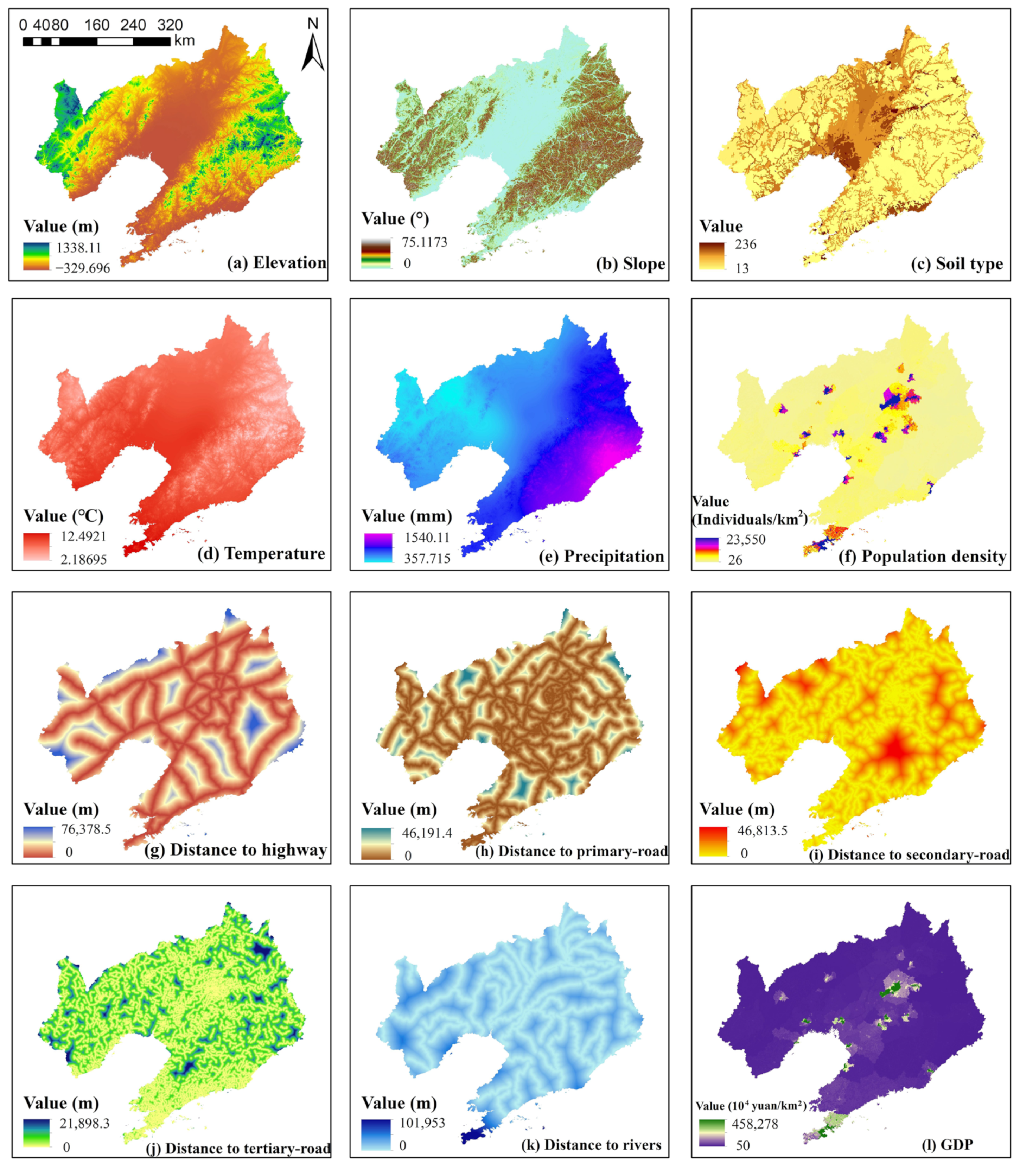
Based on the principles of data accessibility, spatial heterogeneity, consistency, relevance, and quantifiability, with reference to the relevant research literature, elevation, average yearly precipitation, slope, average annual temperature, and soil type were selected as natural drivers; population density, distance to highway, primary road, secondary road, tertiary road, and rivers were selected as social drivers; GDP was selected as the economic driver (Figure 3). Water area is a limiting factor for changing land use.

(2)

The CARS module integrates scenario-driven global land use demand and local land use demand competition effects, as follows:

$$D_k^t=\left\{\begin{array}{c}{D}_k^{t-1} \left(G_k^{t-1}\le G_k^{t-2}\right)\\ D_k^{t-1}\times \frac{G_k^{t-2}}{G_k^{t-1}} \left(G_k^{t-1}<G_k^{t-2}<0\right)\\ D_k^{t-1}\times \frac{G_k^{t-1}}{G_k^{t-2}} \left(0<G_k^{t-2}<G_k^{t-1}\right)\end{array}\right.$$

(5)

where $D_k^t$ and $D_k^{t-1}$ are the adaptive coefficients at time $t$ and $t-1$, respectively, and $G_k^{t-1}$ and $G_k^{t-2}$are the differences between land demand and actual quantity at time $t-1$ and $t-2$, respectively. Equation (6) is as follows:

$$O{P}_{i,k}^{d=1,t}=P_{i,k}^d\times {\Omega }_{i,k}^t\times D_k^t$$

(6)

where $O{P}_{i,k}^{d=1,t}$ is the integrated probability that spatial unit $i$ is at time $t$ when land type $k$ shifts, that is, the overall probability of shifting from the existing land type to type K under the combined influence of growth probabilities, neighborhood effects, and limiting development factors. $P_{i,k}^d$ is the likelihood of suitability of land use at spatial unit $i$ to $k$; ${\Omega }_{i,k}^t$ is the weight of type $k$ in unit $i$ at time t. Equation (7) is as follows:

$$T{P}_{i,k}^{d=1,t}=\left\{\begin{array}{c}{P}_{i,k}^{d=1}\times \left(r\times u_k\right)\times D_k^t \left({\Omega }_{i,k}^t=0, r<P_{i,k}^{d=1}\right)\\ P_{i,k}^{d=1}\times {\Omega }_{i,k}^t\times D_k^t all others\end{array}\right.$$

(7)

where $T{P}_{i,k}^{d=1,t}$is the integrated probability of the transition of spatial unit $i$ to land type $k$ at time $t$ after the introduction of the random patch generation mechanism; $P_{i,k}^{d=1}$ is the likelihood that land use at spatial unit $i$ changes to land use $k$; $r$ is a random number between 0 and 1; $u_k$ represents the threshold of newly generated patches for land type $k$. Equation (8) is as follows:

$$If{{\displaystyle \sum }}_{k=1}^K\left|G_c^{t-1}\right|-{{\displaystyle \sum }}_{k=1}^N\left|G_c^t\right|<step, l=l+1$$

(8)

where $K$ represents the total land types; $step$ represents the step length for fitting the land demand; $l$ indicates the quantity of decay steps. Equation (9) is as follows:

$$\left\{\begin{array}{c} P{d}_{i,c}^{d=1}>\tau T{M}_{k,c}=1 Change\\ P{d}_{i,c}^{d=1}\le \tau T{M}_{k,c}=0 Not change\end{array}\right. \tau ={\delta }^l\times R_1$$

(9)

where $T{M}_{k,c}$ defines whether land type $k$ may be transformed into land type $c$. A value of 1 indicates a permissible transformation, while a value of 0 denotes a restricted transformation; $\delta$ is the attenuation coefficient of the drop threshold $\tau$, $\delta \in \left[0,1\right]$; $R_1$ denotes a normally distributed arbitrary value with a mean of 1. The neighborhood weights are listed in

Table 1. Neighborhood factor parameters.

Land	Cultivated	Forest	Grass	Water	Construction	Unutilized
Weight	0.41	0.42	0.03	0.04	0.09	0.01

[1].

(3)

Accuracy verification analysis. The Kappa coefficient was applied to ensure the accuracy of the PLUS model, as follows [1]:

$$Kappa=\frac{O{A}_o-O{A}_E}{\left(1-O{A}_E\right)}$$

(10)

$$O{A}_O=\frac{{{\displaystyle \sum }}_{k=1}^{6}O{A}_{kk}}{Q}$$

(11)

where $O{A}_O$ is the overall accuracy. $O{A}_E$ represents the likelihood that the simulation results will agree with the real situation; $Q$ represents the total sample quantity, and $O{A}_{kk}$ represents the quantity of samples recognized for type $k$. The Kappa coefficient ranges from −1 to 1. The parameters for each scenario are presented in

Table 2. Parameter setting for multi-scenario simulation of land in 2030.

Scenario	Parameter Setting
Natural development (ND)	The ND scenario continued the change trend from 2010–2020 without any land development strategy constraints and without any adjustment to the model parameters.
Ecological protection (EP)	In the conversion of construction to forest, grass land was permitted, while in the conversion of forest, grass land and water bodies were rigorously limited. Water bodies and forest land are restricted areas. The likelihood of converting forest and grass land to construction land was reduced by 50%, the likelihood of converting cultivated land to construction land was reduced by 30%, and the likelihood of converting cultivated land and grass land to forest land was increased by 30%.
Economic development (ED)	Liaoning Province is China’s main provisionment base. Therefore, the neighborhood weight of cultivated land was increased to 0.7, and that of construction land was increased to 1, denoted as primary and secondary and tertiary development, respectively. Additionally, cultivated land was an economically important land type; it was set as having no transfer to other land types outside construction land and no conversion from construction land to other types in the transfer matrix. The likelihood of converting cultivated land, forest, and grass land to construction land was increased by 20%, and the likelihood of converting construction land to land types other than cultivated land was reduced by 30%.

.

2.3.3. Carbon Storage Analysis

The carbon storage module in the InVEST model was divided into four carbon pools (

Table 3. Carbon densities of each land (t/hm²).

Land	${\mathit{C}}_{\mathit{a}\mathit{b}\mathit{o}\mathit{v}\mathit{e}}$	${\mathit{C}}_{\mathit{b}\mathit{e}\mathit{l}\mathit{o}\mathit{w}}$	${\mathit{C}}_{\mathit{s}\mathit{o}\mathit{i}\mathit{l}}$	${\mathit{C}}_{\mathit{d}\mathit{e}\mathit{a}\mathit{d}}$
Cultivated land	4.75	0	33.51	0
Forest	49.6	24.97	128.67	1.99
Grass	24.38	19.59	52.29	22.74
Water body	2.45	0.62	80.11	0.10
Construction land	4.33	2.17	6.37	0.58
Unused land	0	0	0	0

[55]). Based on previous research results for specific parameter settings [56,57,58,59] the specific equations are as follows [20]:

$$C=C_{above}+C_{below}+C_{soil}+C_{dead}$$

(12)

$$C_{total}={\displaystyle \sum }_{k=1}^6{A}_k\times C_k,\left(k=1,2, \dots ,6\right)$$

(13)

where $C$ is the total carbon storage per cell of each land type, and $C_{above}$, $C_{below}$, $C_{soil}$, and $C_{dead}$ are the aboveground, belowground, soil, and dead carbon densities, respectively. $A_k$ represents the area of each type, and $C_{total}$ represents the entire density of a cell.

2.3.4. Habitat Quality Estimation

Habitat quality represents the effect of human behavior on a precious natural environment [60]. Based on previous research [61,62,63], the parameters were determined (

Table 4. Parameters for threat factors.

Threats	Weight	Max Distance (km)	Spatial Attenuation Types
Cultivated	0.4	5	Exponential
Construction	0.8	12	Linear
Unutilized	0.3	5	Exponential

and

Table 5. Sensitivity parameters of different threats.

Land	Habitat Suitability	Threats
		Cultivated	Construction	Unutilized
Cultivated	0.5	0.3	0.5	0.4
Forest	1.0	0.8	0.9	0.5
Grass	0.7	0.5	0.6	0.7
Water	0.8	0.7	0.9	0.5
Construction	0	0	0	0
Unutilized	0.5	0.4	0.4	0.3

). The formula used is as follows [53]:

$$Q_{xj}=H_{xj}\times \left[1-(\frac{D_{xj}^2}{D_{xj}^2+s^2})\right]$$

(14)

where $Q_{xj}$ denotes the habitat quality of type $j$ in point $x$, $D_{xj}$ denotes the degree of habitat degradation of type $j$ in point $x$, and $s$ denotes the half-saturation constant. $Q_{xj}$ ranges from 0 to 1, with values close to 0 denoting poor habitat quality, and those close to 1 denoting superior habitat quality [64].

2.3.5. Spatial Autocorrelation

Spatial autocorrelation analysis has mostly been employed as a method for the qualitative evaluation of brisk development and vulnerability assessment of eco-environmental systems [44]. Global autocorrelation can provide useful information on connections between geographical objects. Its value is between −1 and 1 [65]. These equations are as follows [43]:

$$Global Mora{n}^{\prime }s I=\frac{T}{S_0}\times \frac{{{\displaystyle \sum }}_{c=1}^T{{\displaystyle \sum }}_{d=1}^T{W}_{cd}\left(Y_c-\overline{Y}\right)\left(Y_d-\overline{Y}\right)}{{{\displaystyle \sum }}_{c=1}^T{\left(Y_c-\overline{Y}\right)}^2}$$

(15)

$$S_0={{\displaystyle \sum }}_{c=1}^T{{\displaystyle \sum }}_{d=1}^T{W}_{cd}$$

(16)

where $I$ represents the global Moran’s index, $T$ is the entire quantity of the sample, and $W_{cd}$ represents the spatial weight matrix. The values for the c-th and d-th samples are represented by $Y_c$ and $Y_d$, respectively, whereas the average value for the area is represented by $\overline{Y}$. $S_0$ is the total amount of spatial weight.

2.3.6. Ecosystem Services Trade-Off/Synergies

Ecosystem services trade-off degree (ESTD) can better clarify the relationship between services [66]. Considering the actual situation, the calculation method of Gong et al. [67] was referred to, assuming $EST{D}_{ij}=EST{D}_{ji}$, that is, the trade-off/synergy was the same for both services by adjusting the order of calculation placement. Equations (17) and (18) are as follows:

$$ESC{I}_1=\frac{E{S}_{1b}-E{S}_{1a}}{E{S}_{1a}}$$

(17)

$$EST{D}_{12}=\frac{1}{2}\left(\frac{ESC{I}_1}{ESC{I}_2}+\frac{ESC{I}_2}{ESC{I}_1}\right)$$

(18)

where $E{S}_{1a}$ and $E{S}_{1b}$ denote the values at time $a$ (initial state) and time $b$ (final state) of the first ecosystem service, respectively; $ESC{I}_1$ and $ESC{I}_2$ denote the ecosystem services change index (ESCI) of the first and second ecosystem services, respectively; $EST{D}_{12}$ is the trade-off degree between the first and second ecosystem services. If $EST{D}_{12}>0$ (or $EST{D}_{12}<0$), then there is a synergistic relationship (or trade-off) between the two ecosystem services. The magnitude of the absolute value reflects the level of trade-offs/synergies.

3. Results

3.1. Land Use Transfer

The land of Liaoning Province had different degrees of transfer in and out between 2010 and 2020 (

Table 6. Land use transfer matrix of 2010–2020 (hectares).

Area	Cultivated	Forest	Grass	Water	Construction	Unutilized	Total M	Total 2010
Cultivated	5,895,848.7	99,746.28	12,113.28	28,977.75	142,295.13	15,761.34		6,194,742.48
M		33.37%	4.05%	9.69%	47.61%	5.27%	100.00%
N		81.92%	52.23%	22.04%	69.24%	27.13%
Forest	96,527.16	5,980,760.73	5133.51	6219.09	27,272.79	2762.91		6,118,676.19
M	69.99%		3.72%	4.51%	19.78%	2.00%	100.00%
N	50.94%		22.14%	4.73%	13.27%	4.76%
Grass	12,756.51	6752.34	441,254.79	2097.09	6894.27	1100.34		470,855.34
M	43.10%	22.81%		7.08%	23.29%	3.72%	100.00%
N	6.73%	5.55%		1.60%	3.35%	1.89%
Water	22,268.61	4734.9	1409.67	407,267.01	25,588.62	38,075.58		499,344.39
M	24.18%	5.14%	1.53%		27.79%	41.35%	100.00%
N	11.75%	3.89%	6.08%		12.45%	65.54%
Construction	41,678.64	9074.34	3666.87	76,951.26	1,062,584.19	395.19		1,194,350.49
M	31.63%	6.89%	2.78%	58.40%		0.30%	100.00%
N	21.99%	7.45%	15.81%	58.53%		0.68%
Unutilized	16,262.55	1447.2	867.69	17,225.73	3470.13	120,348.54		159,621.84
M	41.41%	3.68%	2.21%	43.86%	8.84%		100.00%
N	8.58%	1.19%	3.74%	13.10%	1.69%
Total N	100.00%	100.00%	100.00%	100.00%	100.00%	100.00%
Total 2020	6,085,342.17	6,102,515.79	464,445.81	538,737.93	1,268,105.13	178,443.9		14,637,590.73

). A total of 7.30 $\times$ 10⁵ hectares of land was moved from 2010 to 2020, approximately 4.98% of the total land area. The largest was the shift from cultivated to construction land, with 1.42 $\times$ 10⁵ hectares of cultivated land changing from cultivated to construction land, which was 2.30% of the initial cultivated land area. During the past decade, the likelihood of converting out unutilized land was the highest at 24.60%, while the likelihood of converting out forest land was the smallest, at only 2.25%. From the perspective of transferring in, the conversion of construction land was the largest, at 2.06 $\times$ 10⁵ hectares. The main cause of cultivated land occupation was the rapid development of land scale for construction, with 47.61% of cultivated land being converted for construction. Based on the conversion index $N$, 50.94% of the cultivated land was converted from forestland, indicating that the forest was not adequately protected. Approximately 81.92% of the forest conversion came from cultivated land, 52.23% of the converted grass land came from cultivated land, 58.53% of the transferred area of water bodies was transferred from construction land, 69.24% of the converted area of construction land was transferred from cultivated land, and 65.54% of the converted unutilized land was transferred from water bodies.

3.2. Land Use Driver Detection

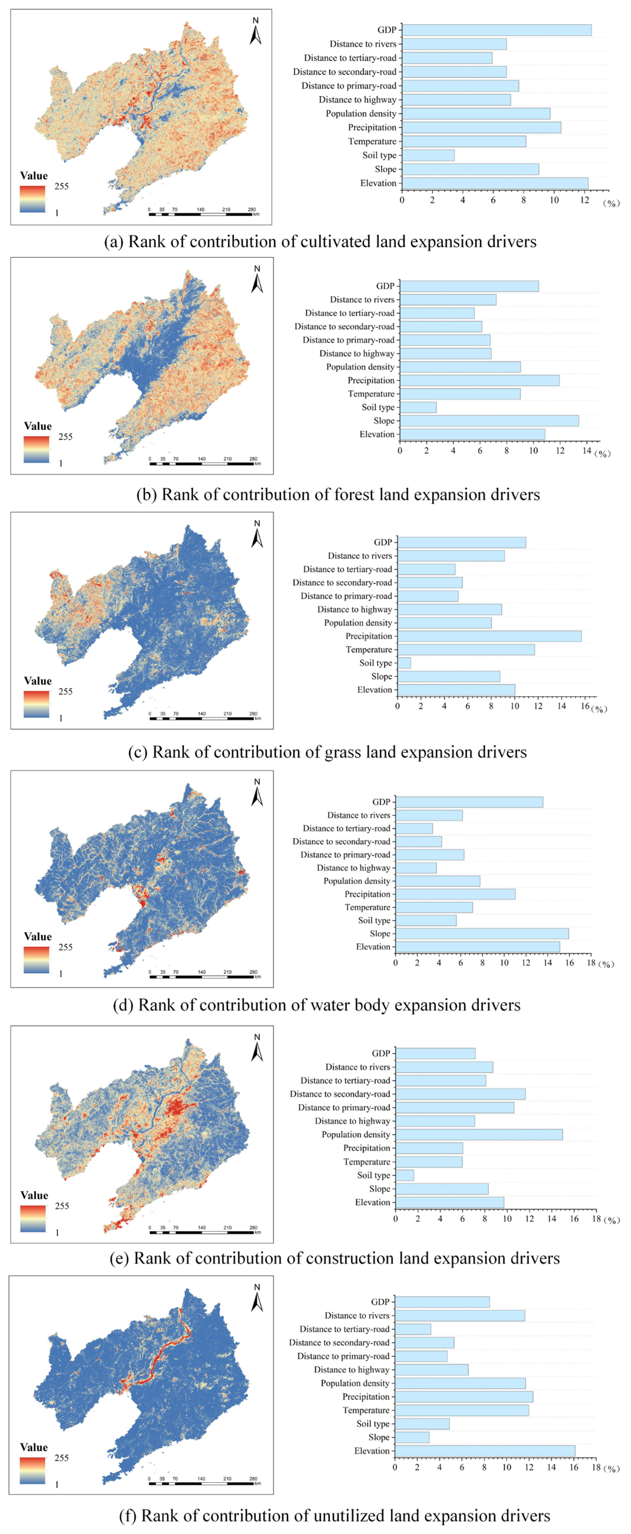
The root mean square errors for cultivated, forest, grassland, water bodies, construction, and unutilized land in Liaoning Province from 2010 to 2030 were 0.144405, 0.126396, 0.058661, 0.0658025, 0.10968, and 0.0364165, respectively, indicating that the data were more credible. The development probability atlas for each category is shown on the left side of Figure 4, and the contribution of each driver to each category is ranked on the right side of Figure 3. GDP and elevation had a greater impact on cultivated land expansion; slope had the greatest effect on forest land expansion; there was a stronger contribution from precipitation and temperature to grassland, a stronger contribution from slope and elevation to water bodies, and a stronger contribution from elevation, precipitation, and temperature to unutilized land, which indicated that the environment’s natural elements are crucial. Population density, distance to secondary roads, and elevation were the key factors affecting the increase in construction land area.

3.3. Land Use Simulation Accuracy Check

Based on the probabilistic land development atlas for 2010–2020, water bodies were used as the restricted conversion area, the neighborhood range was set to 3 by default, the number of parallel threads was set to 6, the decay coefficient of the lowering threshold was set to 0.8, the diffusion coefficient was set to 0.1, and the neighborhood weights, transfer matrix, and land use demand (

Table 7. Multi-scenario land use demand.

Year	Cultivated	Forest	Grass	Water	Construction	Unutilized	Total Number of Rasters
2010	68,795,888	67,964,857	5,232,467	5,318,754	13,051,868	1,771,430	162,135,264
2020	67,584,178	67,786,928	5,157,920	5,701,961	13,923,984	1,980,293	162,135,264
2030 ND	66,508,510	67,603,801	5,090,776	6,080,016	14,687,506	2,164,655	162,135,264
2030 EP	66,626,721	68,163,246	5,104,300	6,080,851	13,995,070	2,165,076	162,135,264
2030 ED	70,186,856	67,497,732	5,062,457	5,849,748	11,376,470	2,162,001	162,135,264

) were input to simulate the land map for 2020. When comparing the prediction results with the actual 2020 data (Figure 5), it was found that the overall accuracy of the PLUS model was 94.16%, the Kappa coefficient was 0.9089, and the simulation results were highly reliable.

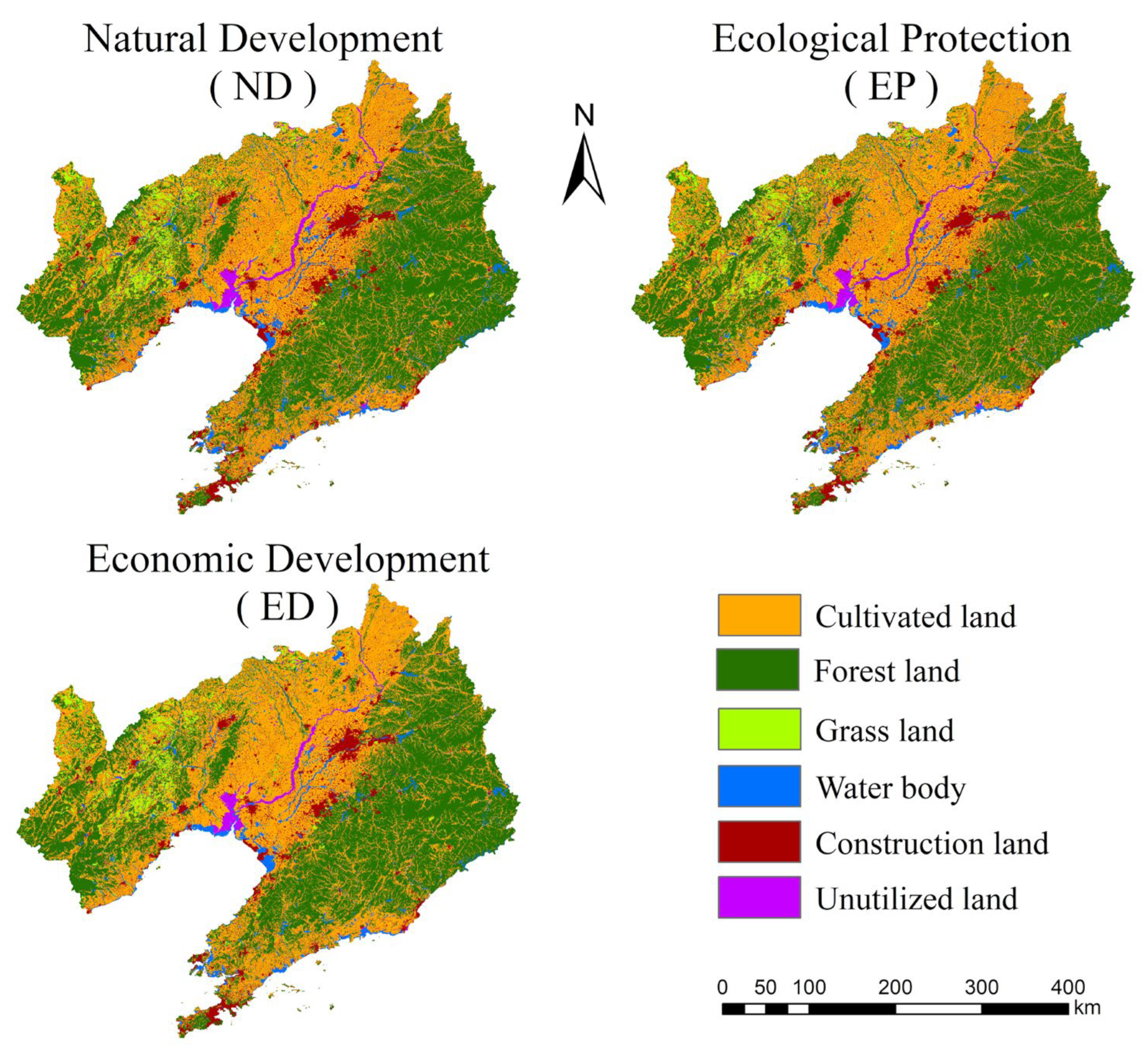
Similarly, based on the 2020 land data, the spatial pattern of land under the three scenarios of ND, EP, and ED in 2030 was further projected (Figure 6).

3.4. Carbon Storage Change

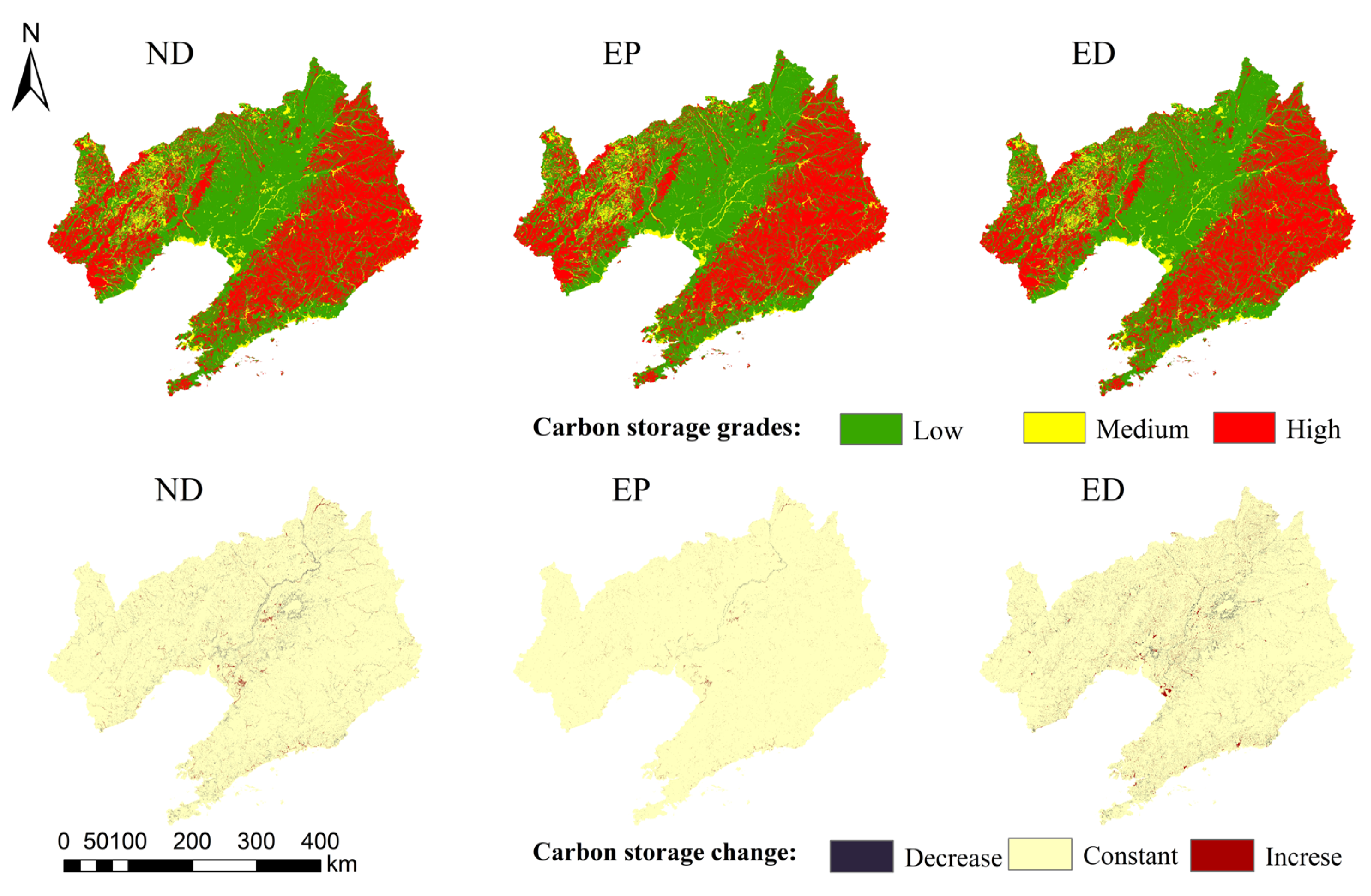
The carbon storage in 2010, 2020, and 2030 was estimated using the carbon storage module (Figure 7). Quantitatively, the total carbon storage values in 2010, 2020, and the ND, EP, and ED scenarios in 2030 were 16.0640 $\times$ 10⁸, 15.9964 $\times$ 10⁸, 15.9558 $\times$ 10⁸, 16.0747 $\times$ 10⁸, and 15.9920 $\times$ 10⁸ Mg/C, respectively. Based on the consideration of grading quality and comparability, this study selected the natural breakpoint method to reclass carbon storage into low- (0 $\le$ value $<$ 3.44), medium- (3.44 $\le$ value $<$ 10.71), and high-value zones (10.71 $\le$ value $<$ 18.47). Spatially, the carbon storage had a certain spatial heterogeneity (Figure 6), with an overall decreasing trend from the northwest and southeast to the middle. Under the ND scenario, the area close to the Liaoning River Basin showed the greatest decline in carbon storage. It was evident that carbon storage increased greatly in the EP scenario, and the ecological environment was improved when compared to the ND and ED scenarios. Under the ED scenario, ecological degradation intensified, and the regions with reduced carbon storage were generally located in the central and northwestern sections of the province; therefore, Liaoning Province should pay more attention to ecological protection while developing its economy in the future.

The carbon storage in Liaoning Province from 2010 to 2030 showed a pattern of co-existence of high, medium, and low values (

Table 8. Area and percentage of carbon storage grades in Liaoning Province from 2010 to 2030 (km²).

Carbon Storage Grades	2010		2020		2030
					ND		EP		ED
	Area	Percent	Area	Percent	Area	Percent	Area	Percent	Area	Percent
Low	75,317.90	51.54	75,140.37	51.49	75,026.40	51.41	74,355.74	50.96	75,556.08	51.78
Medium	9558.51	6.54	9774.76	6.70	10,053.71	6.89	10,220.87	7.00	9619.50	6.59
High	61,248.55	41.92	61,008.40	41.81	60,843.42	41.70	61,346.92	42.04	60,747.96	41.63

), with low- and high-value carbon storage dominating, encompassing more than 50% and 41% of the total area of the research region, respectively. Under the ND scenario, the medium-value region of carbon storage in Liaoning Province gradually expanded in 2030, with an area increase of approximately 278.95 km², while the low- and high-value areas gradually contracted, with area decreases of 113.97 km² and 164.98 km², respectively. In the EP scenario, the size of the low-value area decreased by 784.63 km², while the medium- and high-value areas increased by 446.11 km² and 338.52 km², respectively. Based on the ND scenario, the contraction of the low-value area further expanded, the medium-value area expanded more obviously, and the carbon storage in Liaoning Province was enhanced under the EP scenario. The spatial pattern evolution of the low- and middle-value areas of carbon storage in the ED scenario was completely opposite to that of the ND and EP scenarios, while the spatial pattern evolution of the high-value area was similar to that of the ND scenario, with the low-value area expanding by 415.71 km² and the middle- and high-value areas decreasing by 155.26 km² and 260.44 km², respectively.

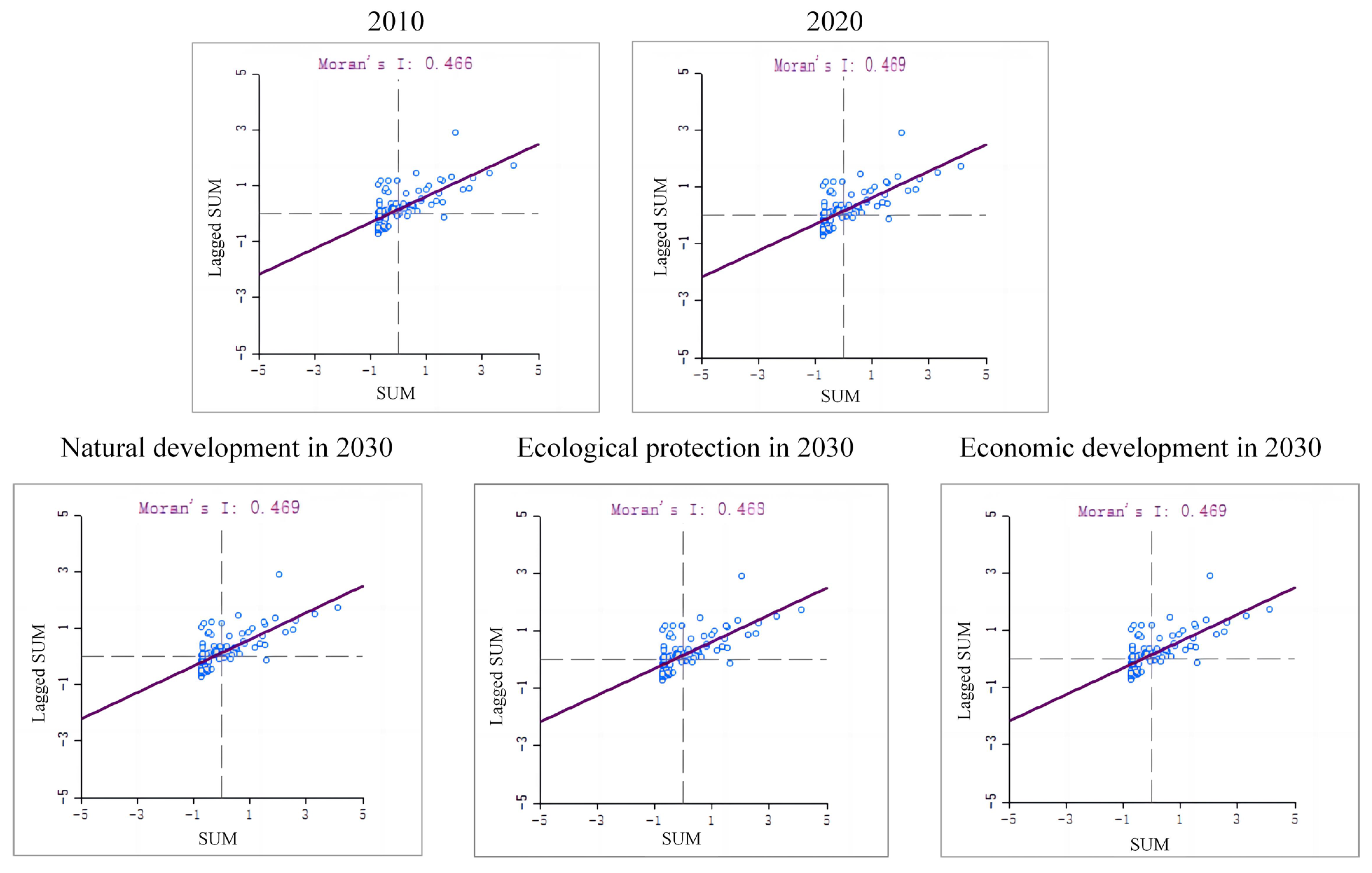
In this study, counties were selected as the research scale, and GeoDa software (v1.2) was used to determine the spatial autocorrelation connections in Liaoning province. The Moran’s I indices of carbon storage in 2010, 2020, and the ND, EP, and ED scenarios in 2030 were 0.466, 0.469, 0.469, 0.468, and 0.469, respectively, all of which were greater than 0, and all showed a positive spatial correlation, that is, the carbon storage within each county in Liaoning Province was not completely random, but rather showed spatial clustering among spatially similar values. Figure 8 shows the majority of the regions to be in the first (the hot-spot region, i.e., high-high clustering) and third quadrants (the cold-spot region, i.e., low-low clustering).

3.5. Habitat Quality Change

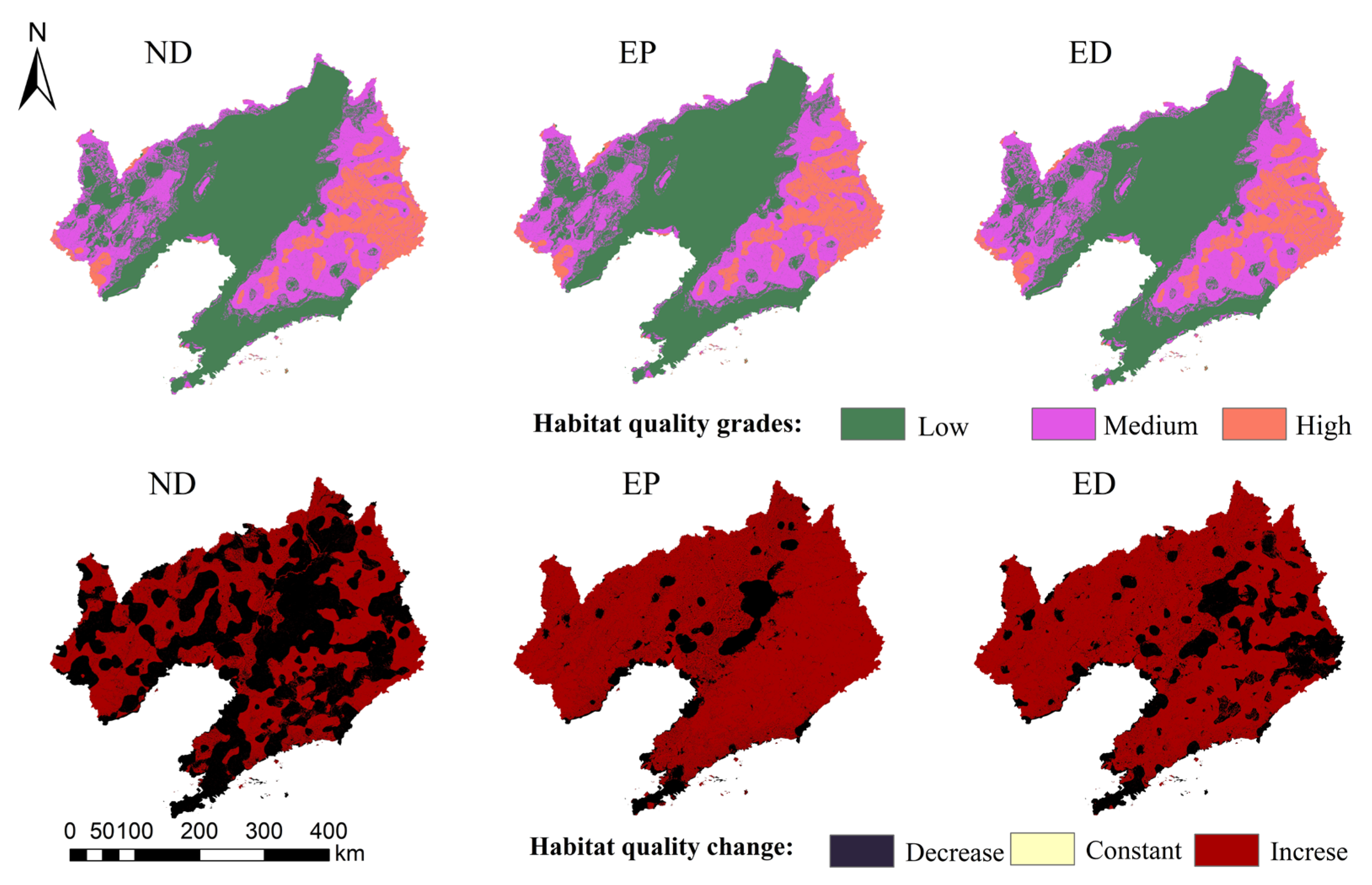
Habitat quality values for Liaoning Province in 2010, 2020, and 2030 were simulated using the habitat quality module. The higher the value, the weaker the intensity of land use development and the better the habitat benefits presented by the land. Based on the consideration of grading quality and comparability, this study used the natural breakpoint method to categorize habitat quality into low- (0 $\le$ value $<$ 0.227451), medium-(0.227451 $\le$ value $<$ 0.545097), and high-value zones (0.545097 $\le$ value $<$ 1). Spatially, the distribution patterns of habitat quality indices displayed some spatial heterogeneity (Figure 9), with an overall rising tendency from the central plain to the northwest and southeast. To better understand the alterations in habitat quality, the raster plots of habitat quality for each scenario in 2020 and 2030 were subtracted separately to obtain different images of habitat quality for each scenario in 2030. Overall, habitat quality changed in most areas, with sporadically unchanged areas. The region with reduced habitat quality grew significantly under the ND scenario, and effective measures to improve habitat quality are urgently needed. Compared with the ND scenario, habitat quality was generally dominated by an increase in the EP and ED scenarios, and habitat quality improved significantly.

Habitat quality indices from 2010 to 2030 showed a pattern of coexisting high, medium, and low values, with low-value habitat quality areas dominating, covering more than 54% of the total area of the study region (

Table 9. Area and percentage of habitat quality grades in Liaoning Province from 2010 to 2030 (km²).

Habitat Quality Grades	2010		2020		2030
					ND		EP		ED
	Area	Percent	Area	Percent	Area	Percent	Area	Percent	Area	Percent
Low	82,757.30	55.88	83,882.95	56.64	83,836.53	56.61	83,206.12	56.18	80,163.63	54.13
Medium	46,352.63	31.30	45,509.11	30.73	45,346.84	30.62	45,368.62	30.63	48,408.31	32.69
High	18,989.83	12.82	18,707.70	12.63	18,916.39	12.77	19,525.02	13.18	19,527.82	13.19

). Under the ND scenario, the region of high habitat quality gradually expanded in 2030, with an area increase of approximately 208.69 km², while the low- and medium-value areas gradually decreased in habitat quality, with area decreases of 46.42 km² and 162.27 km², respectively. Under the EP scenario, the habitat quality pattern showed an evolutionary trend similar to that of the ND scenario, with an increase of 817.32 km² and decreases of 676.83 km² and 140.49 km² in the low- and medium-value areas, respectively. Compared with the ND scenario, the EP scenario showed a more pronounced contraction of the low-value area and an expansion of the high-value area, with the most pronounced improvement in habitat quality. The evolution of low- and high-value areas under the ED scenario was largely in line with those in the ND and EP scenarios, while the spatial pattern evolution of the medium-value area was the opposite of that of the ND and EP scenarios, in which the low-value area decreased the most significantly, by 3719.32 km², and the medium- and high-value areas increased by 2899.20 km² and 820.12 km², respectively. In summary, it could be seen that the habitat quality index in Liaoning Province was sensitive to land [43], and the improvement in habitat quality was more obvious under the EP and ED scenarios in comparison to other scenarios.

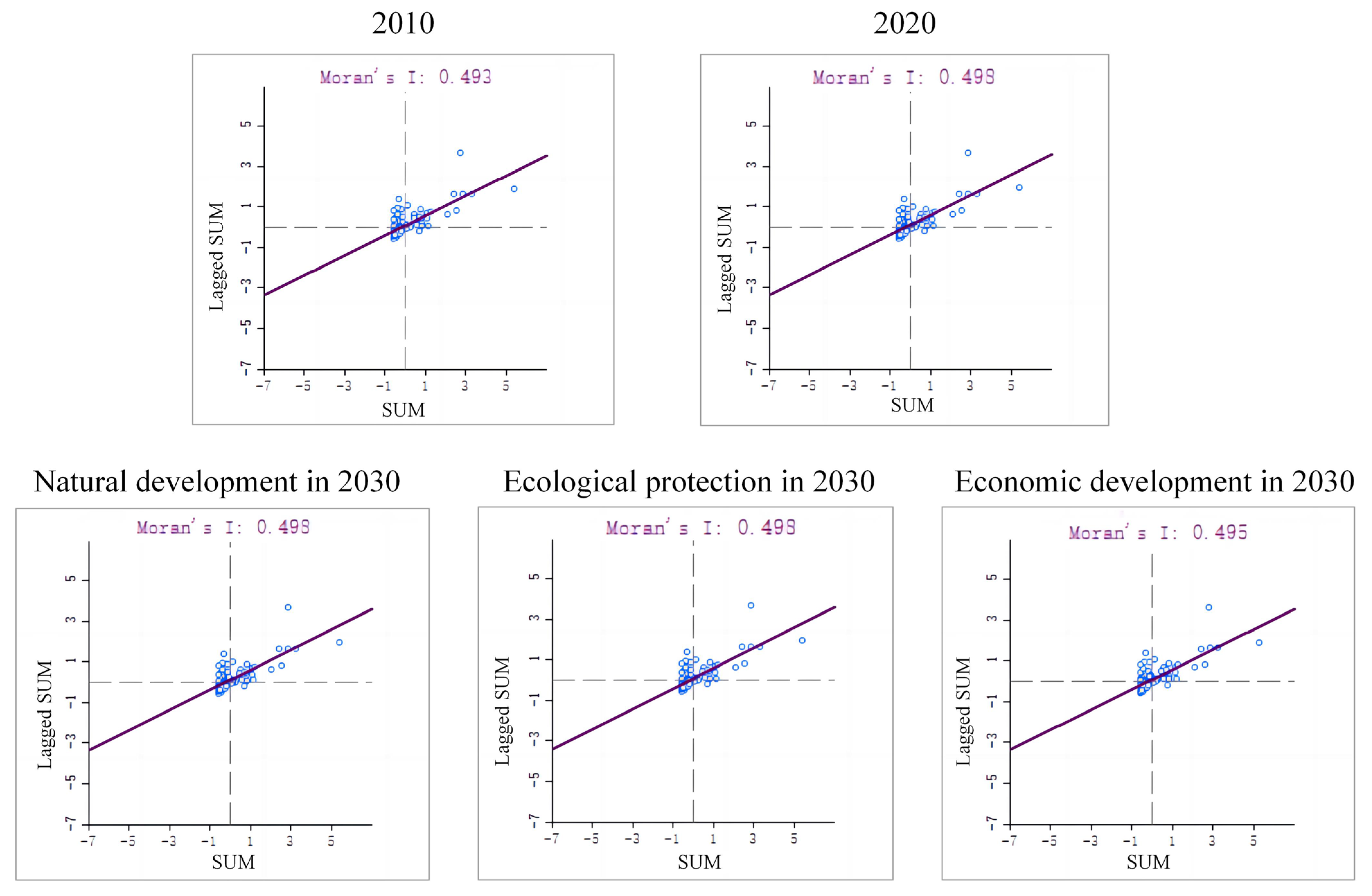
The Moran’s I values of habitat quality in Liaoning Province in 2010, 2020, and the ND, EP, and ED scenarios in 2030 were 0.493, 0.498, 0.498, 0.498, and 0.495, respectively. These values were all greater than 0, that is, habitat quality within each county in Liaoning Province exhibited spatial clustering between spatially similar values. The evolutionary trend of habitat quality correlation was generally similar to that of carbon storage. Habitat quality correlations were enhanced by 0.005 from 2010 to 2020, remained unchanged in 2030 under the ND and ED scenarios, and weakened slightly by 0.003 under the EP scenario. Figure 10 shows that the spatial correlation features of habitat quality and carbon storage in Liaoning Province were basically the same: areas with higher habitat quality tended to be adjacent to areas with higher habitat quality, and areas with lower habitat quality tended to be adjacent to areas with lower habitat quality.

3.6. Carbon Storage and Habitat Quality Trade-Offs and Synergies

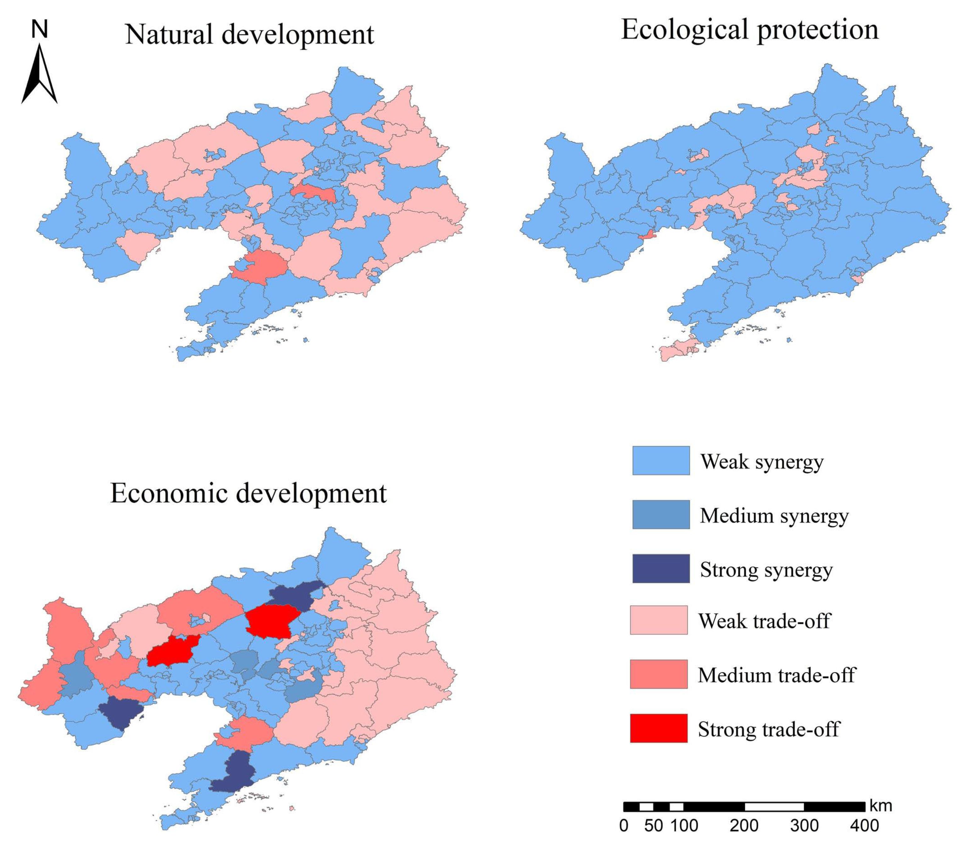
First, the county scale was selected and the effects of habitat quality on carbon storage in 2010, 2020, and 2030 under the ND, EP, and ED scenarios were correlated. To verify the significance of Moran’s I, the pseudo p-value obtained from 999 random permutations in GeoDa using the Monte Carlo simulation was less than 0.05; therefore, Moran’s I could be considered significant and valid. The results showed that habitat quality in Liaoning Province influenced carbon storage to a certain extent. Moran’s I values for habitat quality and carbon storage were 0.458, 0.461, 0.462, 0.461, and 0.463, which were all positive values, indicating that carbon storage and habitat quality were positively correlated in space. Second, the trade-offs and synergies under three development scenarios in 2030 were explored. From the spatial pattern (Figure 11), both trade-off and synergy relationships were widely distributed in the ND scenario, with weak trade-off and synergy dominating. The EP scenario showed weak synergy in most regions and exhibited a weak trade-off in some counties. Strong trade-offs and synergies emerged across counties in the ED scenario, with the central plains and southern coast dominated by synergy, and the northwest and southeast dominated by trade-offs, with more pronounced spatial heterogeneity.

4. Discussion

During 2010–2020, nearly 70% of the area transferred to construction land came from arable land, which may be related to the accelerated urbanization process and the massive encroachment of construction land into non-construction land around the city to meet the needs of urban development. By 2020, 37.42% of the lost arable land was converted into forest and grassland, closely related to the implementation of the local policy of returning farmland to forest. The northwestern and southeastern parts of the study area were clustered with forest and grassland, while the central part was dominated by arable land, along with a high concentration of construction land. The reason for this is that the northwestern and southeastern parts of the study area have higher topography and lower levels of human activity, while the central part is flat and relatively rich in water resources, making it more livable. In addition, this study used the PLUS model to simulate the land use distribution pattern under multiple scenarios in 2030 and used the random forest algorithm to mine the development probability and driving factors of each land use type. Therefore, the LUCC prediction results in this study were only based on maintaining the state of historical trends and applied to subsequent ecosystem service analysis. The simulation accuracy can be further improved if the natural and social drivers are expanded. Although different development scenarios, ND, EP, and ED, were set in this study, there was still a gap between the three types of development pattern sets and the real development scenarios, which cannot cover all future development patterns. Therefore, setting a more realistic amount of future land use demand in conjunction with local policies and narrowing the gap between development scenarios and real development scenarios will become a priority for future land forecast studies.

The northwestern and southeastern regions of Liaoning Province with a higher altitude and high forest density had stronger ecosystem service capacity and gathered areas with high values of carbon storage and habitat quality, and all of them exhibited spatial aggregation between similar values. There were few previous studies on ecosystem services in Liaoning Province, so the results of relevant studies in nearby regions were selected for comparative analysis. Xiang et al. [68] showed the spatial similarity of ecosystem service functions in Northeast China. Mao et al. [69] showed that significant changes in arable and construction land in Northeast China tend to exacerbate landscape fragmentation, which in turn causes a decline in carbon storage and habitat quality. In addition, Wang et al. [70] found that the high-value areas of ecosystem services in Northeast China were mainly distributed in the northwest and southeast from the perspective of ecosystem service valuation, which is consistent with the distribution characteristics of carbon storage and habitat quality in this study. However, the strict implementation of ecological protection will inevitably contradict the need for rapid economic development, and land use optimization is an essential tool for balancing this paradox. Zoning evaluation of the study area in combination with sensitivity can be considered in the future.

This study concluded that the reduction in habitat quality was particularly pronounced around cities and watersheds, that future urban expansion should be reasonably planned and controlled, and that watersheds should be protected to obtain greater ecological benefits. However, there is a lack of scientifically accurate and uniform parameter setting systems when measuring habitat quality; thus, future studies should focus on exploring effective ways to optimize parameter settings. In addition, we identified trade-off and synergy connections between carbon storage and habitat quality in various development scenarios in 2030, which may provide informative implications for decision-making to improve regional sustainability. In recent decades, ecological construction in the Tohoku region has been influenced by numerous national socioeconomic developments and ecological conservation policies, with a national food security program aimed at increasing food production [69] and several ecological conservation projects promoting carbon sequestration and soil conservation [71]. Therefore, future research on multiple ecosystem service functions should consider increasing important service categories, such as water yield, soil conservation, and crop production. Additionally, it is necessary to further explore the reasons for the shift in the synergistic relationship of ecosystem trade-offs, strengthen research on the underlying mechanisms and driving mechanisms, and propose more flexible land management strategies and ecological restoration measures to promote multiple wins among resources, population, economy, and ecology, optimizing ecosystem services, and coordinated regional development.

5. Conclusions

In Liaoning Province, both the pattern of carbon storage and habitat quality revealed a declining trend from the northwest and southeast to the center, and both showed positive spatial correlation. The total carbon storage in 2010, 2020, and the natural development (ND), ecological protection (EP), and economic development (ED) scenarios in 2030 were 16.0640 $\times$ 10⁸, 15.9964 $\times$ 10⁸, 15.9558 $\times$ 10⁸, 16.0747 $\times$ 10⁸, and 15.9920 $\times$ 10⁸ Mg/C, respectively, and were dominated by low- and high-value carbon storage, which encompassed more than 50% and 41% of the total area of the research region, respectively. In addition, habitat quality changed in most areas of Liaoning Province from 2010 to 2030 and was dominated by low-value habitat quality areas, which accounted for 54% of the total research area.

The area of reduced habitat quality area increased dramatically in the ND scenario. Compared to that of the ND scenario, habitat quality in the EP and ED scenarios was generally increasing, and habitat quality improved significantly. In summary, the EP scenario was the only development prospect with increasing total carbon storage, which could increase carbon sequestration by approximately 7.83 $\times$ 10⁶ Mg/C and was also a development prospect with optimal habitat quality. Therefore, the construction of ecological projects to expand the area of high carbon storage value and enhance the regional carbon sequestration capacity can effectively enable Liaoning Province to achieve the goal of “carbon neutrality and carbon peaking”.

Finally, it was found that habitat quality in Liaoning Province influenced carbon storage to some extent, with Moran’s I values of 0.462, 0.461, and 0.463. Weak trade-off and synergy dominated in the ND scenario; most regions showed weak synergy in the EP scenario; spatial heterogeneity became more pronounced in the ED scenario, with strong trade-off and synergy emerging in individual regions. The synergistic area-wide ecosystem services and urban public services have reached a high level and achieved a coordinated development, which is the ultimate goal of sustainable urban development. For trade-off areas, a strict ecological protection system should be implemented in the early stage of urban development, and this should be used as the urban center for urbanization.

References

1. Wang, C.; Li, T.; Guo, X.; Xia, L.; Lu, C.; Wang, C. Plus-InVEST Study of the Chengdu-Chongqing Urban Agglomeration’s Land-Use Change and Carbon Storage. Land 2022, 11, 1617. [Google Scholar] [CrossRef]
2. Yang, Y. Evolution of habitat quality and association with land-use changes in mountainous areas: A case study of the Taihang Mountains in Hebei Province, China. Ecol. Indic. 2021, 129, 107967. [Google Scholar] [CrossRef]
3. Chen, J.; Wang, Y.; Sun, J.; Liang, E.; Shen, M.; Yang, B.; Jia, X.; Zhang, J. Precipitation dominants synergies and trade-offs among ecosystem services across the Qinghai-Tibet Plateau. Glob. Ecol. Conserv. 2021, 32, e01886. [Google Scholar] [CrossRef]
4. Ma, X.; Wang, Z. Progress in the study on the impact of land-use change on regional carbon sources and sinks. Acta Ecol. Sin. 2015, 35, 5898–5907. [Google Scholar]
5. Houghton, R.A.; House, J.I.; Pongratz, J.; Van Der Werf, G.R.; Defries, R.S.; Hansen, M.C.; Le Quéré, C.; Ramankutty, N. Carbon emissions from land use and land-cover change. Biogeosciences 2012, 9, 5125–5142. [Google Scholar] [CrossRef] [Green Version]
6. Piao, S.; Yue, C.; Ding, J.; Guo, Z. Perspectives on the role of terrestrial ecosystems in the ‘carbon neutrality’strategy. Sci. China Earth Sci. 2022, 65, 1178–1186. [Google Scholar] [CrossRef]
7. Yu, Z.; Ciais, P.; Piao, S.; Houghton, R.A.; Lu, C.; Tian, H.; Agathokleous, E.; Kattel, G.R.; Sitch, S.; Goll, D. Forest expansion dominates China’s land carbon sink since 1980. Nat. Commun. 2022, 13, 5374. [Google Scholar] [CrossRef]
8. Foley, J.A.; DeFries, R.; Asner, G.P.; Barford, C.; Bonan, G.; Carpenter, S.R.; Chapin, F.S.; Coe, M.T.; Daily, G.C.; Gibbs, H.K. Global consequences of land use. Science 2005, 309, 570–574. [Google Scholar] [CrossRef] [Green Version]
9. Wang, L.; Zhu, R.; Yin, Z.; Chen, Z.; Fang, C.; Lu, R.; Zhou, J.; Feng, Y. Impacts of Land-Use Change on the Spatio-Temporal Patterns of Terrestrial Ecosystem Carbon Storage in the Gansu Province, Northwest China. Remote Sens. 2022, 14, 3164. [Google Scholar] [CrossRef]
10. Fellman, J.B.; Hood, E.; Dryer, W.; Pyare, S. Stream physical characteristics impact habitat quality for Pacific salmon in two temperate coastal watersheds. PloS ONE 2015, 10, e0132652. [Google Scholar] [CrossRef] [Green Version]
11. McKinney, M.L. Urbanization, Biodiversity, and ConservationThe impacts of urbanization on native species are poorly studied, but educating a highly urbanized human population about these impacts can greatly improve species conservation in all ecosystems. Bioscience 2002, 52, 883–890. [Google Scholar] [CrossRef]
12. Wu, J.; Luo, J.; Zhang, H.; Qin, S.; Yu, M. Projections of land use change and habitat quality assessment by coupling climate change and development patterns. Sci. Total Environ. 2022, 847, 157491. [Google Scholar] [CrossRef]
13. La Rosa, D.; Spyra, M.; Inostroza, L. Indicators of Cultural Ecosystem Services for urban planning: A review. Ecol. Indic. 2016, 61, 74–89. [Google Scholar] [CrossRef]
14. Wainger, L.A.; King, D.M.; Mack, R.N.; Price, E.W.; Maslin, T. Can the concept of ecosystem services be practically applied to improve natural resource management decisions? Ecol. Econ. 2010, 69, 978–987. [Google Scholar] [CrossRef]
15. Sun, X.; Crittenden, J.C.; Li, F.; Lu, Z.; Dou, X. Urban expansion simulation and the spatio-temporal changes of ecosystem services, a case study in Atlanta Metropolitan area, USA. Sci. Total Environ. 2018, 622, 974–987. [Google Scholar] [CrossRef]
16. Thom, D.; Seidl, R. Natural disturbance impacts on ecosystem services and biodiversity in temperate and boreal forests. Biol. Rev. 2016, 91, 760–781. [Google Scholar] [CrossRef]
17. Lyu, R.; Zhang, J.; Xu, M.; Li, J. Impacts of urbanization on ecosystem services and their temporal relations: A case study in Northern Ningxia, China. Land Use Policy 2018, 77, 163–173. [Google Scholar] [CrossRef]
18. He, J.; Huang, J.; Li, C. The evaluation for the impact of land use change on habitat quality: A joint contribution of cellular automata scenario simulation and habitat quality assessment model. Ecol. Model. 2017, 366, 58–67. [Google Scholar] [CrossRef]
19. Trevathan-Tackett, S.M.; Wessel, C.; Cebrián, J.; Ralph, P.J.; Masqué, P.; Macreadie, P.I. Effects of small-scale, shading-induced seagrass loss on blue carbon storage: Implications for management of degraded seagrass ecosystems. J. Appl. Ecol. 2018, 55, 1351–1359. [Google Scholar] [CrossRef]
20. Zhao, M.; He, Z.; Du, J.; Chen, L.; Lin, P.; Fang, S. Assessing the effects of ecological engineering on carbon storage by linking the CA-Markov and InVEST models. Ecol. Indic. 2019, 98, 29–38. [Google Scholar] [CrossRef]
21. Wang, Y.; Dai, E. Spatial-temporal changes in ecosystem services and the trade-off relationship in mountain regions: A case study of Hengduan Mountain region in Southwest China. J. Clean. Prod. 2020, 264, 121573. [Google Scholar] [CrossRef]
22. Bhagabati, N.K.; Ricketts, T.; Sulistyawan, T.B.S.; Conte, M.; Ennaanay, D.; Hadian, O.; McKenzie, E.; Olwero, N.; Rosenthal, A.; Tallis, H. Ecosystem services reinforce Sumatran tiger conservation in land use plans. Biol. Conserv. 2014, 169, 147–156. [Google Scholar] [CrossRef]
23. Bagstad, K.J.; Johnson, G.W.; Voigt, B.; Villa, F. Spatial dynamics of ecosystem service flows: A comprehensive approach to quantifying actual services. Ecosyst. Serv. 2013, 4, 117–125. [Google Scholar] [CrossRef]
24. Sherrouse, B.C.; Clement, J.M.; Semmens, D.J. A GIS application for assessing, mapping, and quantifying the social values of ecosystem services. Appl. Geogr. 2011, 31, 748–760. [Google Scholar] [CrossRef]
25. Wang, Z.; Zeng, J.; Chen, W. Impact of urban expansion on carbon storage under multi-scenario simulations in Wuhan, China. Environ. Sci. Pollut. Res. 2022, 29, 45507–45526. [Google Scholar] [CrossRef]
26. He, C.; Zhang, D.; Huang, Q.; Zhao, Y. Assessing the potential impacts of urban expansion on regional carbon storage by linking the LUSD-urban and InVEST models. Environ. Model. Softw. 2016, 75, 44–58. [Google Scholar] [CrossRef]
27. Yan, J.; Wang, L.; He, H.; Liang, D.; Song, W.; Han, W. Large-Area Land-Cover Changes Monitoring With Time-Series Remote Sensing Images Using Transferable Deep Models. IEEE Trans. Geosci. Remote Sens. 2022, 60, 1–17. [Google Scholar] [CrossRef]
28. Yang, R.; Chen, H.; Chen, S.; Ye, Y. Spatiotemporal evolution and prediction of land use/land cover changes and ecosystem service variation in the Yellow River Basin, China. Ecol. Indic. 2022, 145, 109579. [Google Scholar] [CrossRef]
29. Buya, S.; Tongkumchum, P.; Owusu, B.E. Modelling of land-use change in Thailand using binary logistic regression and multinomial logistic regression. Arab. J. Geosci. 2020, 13, 437. [Google Scholar] [CrossRef]
30. Zeng, B.; Duan, H.; Zhou, Y. A new multivariable grey prediction model with structure compatibility. Appl. Math. Model. 2019, 75, 385–397. [Google Scholar] [CrossRef]
31. Huang, Y.; Nian, P.; Zhang, W. The prediction of interregional land use differences in Beijing: A Markov model. Environ. Earth Sci. 2015, 73, 4077–4090. [Google Scholar] [CrossRef]
32. Saputra, M.H.; Lee, H.S. Prediction of land use and land cover changes for north sumatra, indonesia, using an artificial-neural-network-based cellular automaton. Sustainability 2019, 11, 3024. [Google Scholar] [CrossRef] [Green Version]
33. Wu, F.; Webster, C.J. Simulation of land development through the integration of cellular automata and multicriteria evaluation. Environ. Plan. B Plan. Des. 1998, 25, 103–126. [Google Scholar] [CrossRef]
34. Omrani, H.; Parmentier, B.; Helbich, M.; Pijanowski, B. The land transformation model-cluster framework: Applying k-means and the Spark computing environment for large scale land change analytics. Environ. Model. Softw. 2019, 111, 182–191. [Google Scholar] [CrossRef]
35. Chotchaiwong, P.; Wijitkosum, S. Predicting urban expansion and urban land use changes in Nakhon Ratchasima City using a CA-Markov model under two different scenarios. Land 2019, 8, 140. [Google Scholar] [CrossRef] [Green Version]
36. Wang, N.; Chen, X.; Zhang, Z.; Pang, J. Spatiotemporal dynamics and driving factors of county-level carbon storage in the Loess Plateau: A case study in Qingcheng County, China. Ecol. Indic. 2022, 144, 109460. [Google Scholar] [CrossRef]
37. Wang, R.; Bai, Y.; Alatalo, J.M.; Yang, Z.; Yang, Z.; Yang, W.; Guo, G. Impacts of rapid urbanization on ecosystem services under different scenarios–A case study in Dianchi Lake Basin, China. Ecol. Indic. 2021, 130, 108102. [Google Scholar] [CrossRef]
38. Sohl, T.L.; Claggett, P.R. Clarity versus complexity: Land-use modeling as a practical tool for decision-makers. J. Environ. Manag. 2013, 129, 235–243. [Google Scholar] [CrossRef]
39. Meentemeyer, R.K.; Tang, W.; Dorning, M.A.; Vogler, J.B.; Cunniffe, N.J.; Shoemaker, D.A. FUTURES: Multilevel simulations of emerging urban–rural landscape structure using a stochastic patch-growing algorithm. Ann. Assoc. Am. Geogr. 2013, 103, 785–807. [Google Scholar] [CrossRef] [Green Version]
40. Yang, J.; Gong, J.; Tang, W.; Liu, C. Patch-based cellular automata model of urban growth simulation: Integrating feedback between quantitative composition and spatial configuration. Comput. Environ. Urban Syst. 2020, 79, 101402. [Google Scholar] [CrossRef]
41. Liang, X.; Liu, X.; Chen, G.; Leng, J.; Wen, Y.; Chen, G. Coupling fuzzy clustering and cellular automata based on local maxima of development potential to model urban emergence and expansion in economic development zones. Int. J. Geogr. Inf. Sci. 2020, 34, 1930–1952. [Google Scholar] [CrossRef]
42. Liang, X.; Guan, Q.; Clarke, K.C.; Liu, S.; Wang, B.; Yao, Y. Understanding the drivers of sustainable land expansion using a patch-generating land use simulation (PLUS) model: A case study in Wuhan, China. Comput. Environ. Urban Syst. 2021, 85, 101569. [Google Scholar] [CrossRef]
43. Ren, D.; Cao, A. Analysis of the heterogeneity of landscape risk evolution and driving factors based on a combined GeoDa and Geodetector model. Ecol. Indic. 2022, 144, 109568. [Google Scholar] [CrossRef]
44. Wu, Z.; Zhang, F.; Di, D.; Wang, H. Study of spatial distribution characteristics of river eco-environmental values based on emergy-GeoDa method. Sci. Total Environ. 2022, 802, 149679. [Google Scholar] [CrossRef] [PubMed]
45. Nero, B.F.; Callo-Concha, D.; Anning, A.; Denich, M. Urban green spaces enhance climate change mitigation in cities of the global south: The case of Kumasi, Ghana. Procedia Eng. 2017, 198, 69–83. [Google Scholar] [CrossRef]
46. Wahyudi, A.A.J.; Afdal. Climate change mitigation: From carbon cycle to policy. In AIP Conference Proceedings; AIP Publishing: Melville, NY, USA, 2018; p. 040019. [Google Scholar]
47. The Ministry of Natural Resources Standard Map Service. Available online: http://bzdt.ch.mnr.gov.cn/ (accessed on 17 February 2023).
48. Resource and Environment Science and Data Center. Available online: https://www.resdc.cn/ (accessed on 1 December 2022).
49. Hu, W.; Li, G.; Gao, Z.; Jia, G.; Wang, Z.; Li, Y. Assessment of the impact of the Poplar Ecological Retreat Project on water conservation in the Dongting Lake wetland region using the InVEST model. Sci. Total Environ. 2020, 733, 139423. [Google Scholar] [CrossRef]
50. National Geomatics Center of China. Available online: http://www.ngcc.cn/ngcc/ (accessed on 4 December 2022).
51. OpenStreetMap. Available online: http://www.openstreetmap.org/ (accessed on 4 December 2022).
52. Li, X.; Liu, Z.; Li, S.; Li, Y. Multi-Scenario Simulation Analysis of Land Use Impacts on Habitat Quality in Tianjin Based on the PLUS Model Coupled with the InVEST Model. Sustainability 2022, 14, 6923. [Google Scholar] [CrossRef]
53. Wei, Q.; Abudureheman, M.; Halike, A.; Yao, K.; Yao, L.; Tang, H.; Tuheti, B. Temporal and spatial variation analysis of habitat quality on the PLUS-InVEST model for Ebinur Lake Basin, China. Ecol. Indic. 2022, 145, 109632. [Google Scholar] [CrossRef]
54. Li, X.; Fu, J.; Jiang, D.; Lin, G.; Cao, C. Land use optimization in Ningbo City with a coupled GA and PLUS model. J. Clean. Prod. 2022, 375, 134004. [Google Scholar] [CrossRef]
55. Zhu, L.; Ke, H.U.; Shuang, S.; Yuhan, L.; Jiaxin, L. Research on the Spatiotemporal Variation of Carbon Storage in the Costal Zone of Liaoning Province Based on InVEST Model. Geoscience 2021, 36, 96. (In Chinese) [Google Scholar] [CrossRef]
56. Li, H.; Pei, J.; Wang, J.; Li, S.; Gao, G. Organic carbon density and storage of the major black soil regions in Northeast China. J. Soil Sci. Plant Nutr. 2013, 13, 883–893. [Google Scholar] [CrossRef]
57. Li, X.; Huang, C.; Jin, H.; Han, Y.; Kang, S.; Liu, J.; Cai, H.; Hu, T.; Yang, G.; Yu, H. Spatio-Temporal Patterns of Carbon Storage Derived Using the InVEST Model in Heilongjiang Province, Northeast China. Ecol. Impacts Degrad. Permafr. 2022, 10, 846456. [Google Scholar] [CrossRef]
58. Li, Y.; Liu, Z.; Li, S.; Li, X. Multi-Scenario Simulation Analysis of Land Use and Carbon Storage Changes in Changchun City Based on FLUS and InVEST Model. Land 2022, 11, 647. [Google Scholar] [CrossRef]
59. Xiang, H.; Jia, M.; Wang, Z.; Li, L.; Mao, D.; Zhang, D.; Cui, G.; Zhu, W. Impacts of land cover changes on ecosystem carbon stocks over the transboundary Tumen River Basin in Northeast Asia. Chin. Geogr. Sci. 2018, 28, 973–985. [Google Scholar] [CrossRef] [Green Version]
60. Wang, B.; Cheng, W. Effects of Land Use/Cover on Regional Habitat Quality under Different Geomorphic Types Based on InVEST Model. Remote Sens. 2022, 14, 1279. [Google Scholar] [CrossRef]
61. Bai, L.; Xiu, C.; Feng, X.; Liu, D. Influence of urbanization on regional habitat quality: A case study of Changchun City. Habitat Int. 2019, 93, 102042. [Google Scholar] [CrossRef]
62. Dai, L.; Li, S.; Lewis, B.J.; Wu, J.; Yu, D.; Zhou, W.; Zhou, L.; Wu, S. The influence of land use change on the spatial–temporal variability of habitat quality between 1990 and 2010 in Northeast China. J. For. Res. 2019, 30, 2227–2236. [Google Scholar] [CrossRef]
63. Yu, W.; Ji, R.; Han, X.; Chen, L.; Feng, R.; Wu, J.; Zhang, Y. Evaluation of the biodiversity conservation function in Liaohe Delta wetland, northeastern China. J. Meteorol. Res. 2020, 34, 798–805. [Google Scholar] [CrossRef]
64. Chiang, L.-C.; Lin, Y.-P.; Huang, T.; Schmeller, D.S.; Verburg, P.H.; Liu, Y.-L.; Ding, T.-S. Simulation of ecosystem service responses to multiple disturbances from an earthquake and several typhoons. Landsc. Urban Plan. 2014, 122, 41–55. [Google Scholar] [CrossRef]
65. Anselin, L. From SpaceStat to CyberGIS: Twenty years of spatial data analysis software. Int. Reg. Sci. Rev. 2012, 35, 131–157. [Google Scholar] [CrossRef]
66. Zhang, X.; Xie, H.; Shi, J.; Lv, T.; Zhou, C.; Liu, W. Assessing changes in ecosystem service values in response to land cover dynamics in Jiangxi Province, China. Int. J. Environ. Res. Public Health 2020, 17, 3018. [Google Scholar] [CrossRef] [PubMed]
67. Gong, J.; Liu, D.; Zhang, J.; Xie, Y.; Cao, E.; Li, H. Tradeoffs/synergies of multiple ecosystem services based on land use simulation in a mountain-basin area, western China. Ecol. Indic. 2019, 99, 283–293. [Google Scholar] [CrossRef]
68. Xiang, H.; Zhang, J.; Mao, D.; Wang, Z.; Qiu, Z.; Yan, H. Identifying spatial similarities and mismatches between supply and demand of ecosystem services for sustainable Northeast China. Ecol. Indic. 2022, 134, 108501. [Google Scholar] [CrossRef]
69. Mao, D.; He, X.; Wang, Z.; Tian, Y.; Xiang, H.; Yu, H.; Man, W.; Jia, M.; Ren, C.; Zheng, H. Diverse policies leading to contrasting impacts on land cover and ecosystem services in Northeast China. J. Clean. Prod. 2019, 240, 117961. [Google Scholar] [CrossRef]
70. Wang, X.; Pan, T.; Pan, R.; Chi, W.; Ma, C.; Ning, L.; Wang, X.; Zhang, J. Impact of land transition on landscape and ecosystem service value in Northeast Region of China from 2000–2020. Land 2022, 11, 696. [Google Scholar] [CrossRef]
71. Ouyang, Z.; Zheng, H.; Xiao, Y.; Polasky, S.; Liu, J.; Xu, W.; Wang, Q.; Zhang, L.; Xiao, Y.; Rao, E. Improvements in ecosystem services from investments in natural capital. Science 2016, 352, 1455–1459. [Google Scholar] [CrossRef]
Figure 1. Flowchart of our study.
Sustainability 15 04500 g001
Figure 2. Topography of Liaoning Province.
Sustainability 15 04500 g002
Figure 3. Spatial pattern of driving factors affecting land use.
Sustainability 15 04500 g003
Figure 4. Ranking of the driving forces affecting land expansion.
Sustainability 15 04500 g004
Figure 5. A check of the simulation accuracy of spatial distribution patterns in 2020.
Sustainability 15 04500 g005
Figure 6. Predicted results in Liaoning Province under three scenarios in 2030.
Sustainability 15 04500 g006
Figure 7. Prediction and changes in carbon storage under three scenarios.
Sustainability 15 04500 g007
Figure 8. Moran scatter plot of carbon storage.
Sustainability 15 04500 g008
Figure 9. Prediction and changes in habitat quality under three scenarios.
Sustainability 15 04500 g009
Figure 10. Moran scatter plot of habitat quality.
Sustainability 15 04500 g010
Figure 11. Trade-offs and synergies of carbon storage and habitat quality under three scenarios from 2020 to 2030.
Sustainability 15 04500 g011