Road-Section-Based Analysis of Vehicle Emissions and Energy Consumption

Sunhee Jang; Ki-Han Song; Daejin Kim; Joonho Ko; Seongkwan Mark Lee; Sabeur Elkosantini; Wonho Suh

doi:10.3390/su15054421

,

and

¹

Department of Smart City Engineering, Hanyang University ERICA Campus, Ansan 15588, Republic of Korea

²

Department of Civil Engineering, Seoul National University of Science and Technology, Seoul 01811, Republic of Korea

³

Asia Pacific School of Logistics, Graduate School of Logistics, Inha University, 100 Inha-ro, Michuhol-gu, Incheon 22212, Republic of Korea

⁴

Graduate School of Urban Studies, Hanyang University, Seoul 04763, Republic of Korea

Sustainability2023, 15(5), 4421;https://doi.org/10.3390/su15054421

This article belongs to the Special Issue Selected Papers on Sustainability from IMETI 2022

Version Notes

Order Reprints

Abstract

To monitor air pollution on roads in urban areas, it is necessary to accurately estimate emissions from vehicles. For this purpose, vehicle emission estimation models have been developed. Vehicle emission estimation models are categorized into macroscopic models and microscopic models. While the calculation is simple, macroscopic models utilize the average speed of vehicles without accounting for the acceleration and deceleration of individual vehicles. Therefore, limitations exist in estimating accurate emissions when there are frequent changes in driving behavior. Microscopic emission estimation models overcome these limitations by utilizing the trajectory data of each vehicle. In this method, the total emissions in a road segment are calculated by adding together the emissions from individual vehicles. However, most research studies consider the total vehicle emissions in a road section without considering the difference in vehicle emissions at different locations of a selected road section. In this study, a road segment between two intersections was divided into sub-sections, and energy consumption and emission generation were analyzed. Since there are unique driving behaviors depending on the section of the road segment, energy consumption and emission generation patterns were identified. The findings of this study are expected to provide more detailed and quantitative data for better modeling of energy consumption and emissions in urban areas.

Keywords:

MOVES; emission; energy; signalized intersection; sub-section; microscopic analysis

1. Introduction

At signalized intersections in urban areas, large amounts of emissions are generated due to frequent vehicle stops and delays, so air pollution management is required [1,2]. In air pollution mitigation plans, it is necessary to estimate accurate vehicle emissions generated at signalized intersections. Recent studies have been conducted to calculate and monitor emissions at signalized intersections using vehicle emission estimation models [3,4,5]. Vehicle emission estimation models are categorized into macroscopic models and microscopic models. While the calculation is simple, macroscopic models utilize the average speed of vehicles without accounting for the acceleration and deceleration of individual vehicles. Therefore, limitations exist in estimating accurate emissions when there are frequent changes in driving behavior [6,7,8]. Microscopic emission estimation models overcome these limitations by utilizing the trajectory data of each vehicle. In this method, the total emission amount in a road segment is calculated by adding together the emissions from individual vehicles.

However, most research studies consider the total vehicle emissions in a road section without considering the difference in vehicle emissions at different locations of a selected road section. At signalized intersections, vehicles often change their driving behavior due to traffic signals [9,10]. For example, driving behavior before a signal is different from driving behavior after a signal, resulting in different emission and energy consumption patterns [11]. In addition, emissions increase during acceleration, deceleration, and stopping compared with constant-speed driving. Additionally, driving behavior depends on traffic conditions [12]. In this study, a road segment between two intersections was divided into sub-sections, and energy consumption and emission generation were analyzed. Since there are unique driving behaviors depending on the section of a road segment, energy consumption and emission generation patterns were identified. In this paper, vehicle emissions and energy consumption in each sub-section were compared. Correlations between traffic flow characteristics and emissions were analyzed. A cluster analysis of emissions by sub-section was also conducted. Xu et al. (2016) integrated VISSIM simulations with MOVES to analyze the sensitivity of emissions to simulation parameters. They found that emissions are sensitive to the vehicle type distribution in the fleet. It was also found that the range of the look-ahead distance in the car-following model and the range of the accepted deceleration rate can impact emissions [13]. Hatem Abou-Senna (2013) integrated a micro-traffic simulation model with the latest US Environmental Protection Agency mobile source emissions. He estimated CO₂ emissions based on vehicle operation data expressed in seconds [14,15]. Haobing Liu (2019) analyzed traffic simulations, the MOVES emission inventory, and the AERMOD dispersion model. He explored the impacts of three alternative truck shifting strategies on PM_2.5 emissions and concentrations [16]. Lim et al. (2005) analyzed factors affecting vehicle emissions and suggested that different methodologies provide different outputs depending on the level of traffic volume [17]. Kim et al. (2012) suggested that different models should be applied according to the type of road facilities. In addition, they suggested that different emission parameters should be applied according to traffic conditions [18]. Heo et al. (2020) proposed a link-based method for estimating microscopic emissions and suggested that microscopic emissions and macroscopic emissions show a large difference [6,7]. Yunlong et al. (2022) analyzed emissions and energy consumption according to different driving behaviors and suggested the existence of an emission reduction effect due to eco-driving [19]. Christos et al. (2019) analyzed the emissions and energy consumption of aggressive driving at signalized intersections and suggested that higher emissions are due to higher acceleration/deceleration [20]. Shaheen et al. (2015) utilized a microscopic estimation model to analyze the effect of reducing the emissions and energy consumption of autonomous vehicles. They suggested that emissions can be reduced thanks to the platooning of autonomous vehicles [21]. Fangfang et al. (2017) analyzed emissions and energy consumption at a signalized intersection. They found that driving with lower acceleration/deceleration deviation results in lower emissions and energy consumption [22].

Relevant studies in the literature have mainly analyzed vehicle emissions according to driving behavior. However, not many studies have focused on the difference in vehicle emissions at different locations of a selected road section. In this study, a road segment between two intersections was divided into sub-sections, and energy consumption and emission generation were analyzed.

2. Methodology

In this study, an arterial road network was established using VISSIM. Second-by-second trajectory data of individual vehicles were extracted using VISSIM COM [23,24]. Vehicle emissions in each sub-section were calculated using the MOVES OP mode.

OpMode is a method for estimating micro-emissions by classifying vehicle trajectory data values expressed in seconds into 23 operating modes based on velocity, acceleration, and VSP (vehicle-specific power). Using MOVES Tool to analyze emissions from multiple vehicles necessitates a long calculation time, so the MOVES-Matrix method can be used as an alternative. MOVES-Matrix is a model developed by the Georgia Institute of Technology research team. It presents the same results as MOVES, and calculations are performed 200 times faster than when using the MOVES model. MOVES-Matrix is a method to minimize excessive calculation time by calculating emission factors per unit length and unit time according to road environment, vehicle type, and vehicle model year using MOVES. In this study, emissions were calculated by multiplying the calculated emission factor, traffic volume, and section length. Figure 1 shows the analysis process of this study.

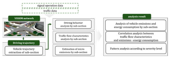
Figure 1. Analysis process.

In previous studies, microscopic emission analysis has mainly been conducted by estimating the total emission amount by calculating the ratio of driving behavior in all sections. With the total micro-emission estimation method, the total amount of micro-emissions can be obtained by calculating the operating mode ratio using the acceleration and deceleration data of vehicles passing through the entire section [25,26,27,28]. However, when estimating the total emissions, the emissions in the entire section are counted as one, so there is a limit to deriving the emissions and energy consumption generated in a specific part of the road.

In addition, there is a limit to not considering the change in the driving behavior of vehicles within the intersection and the difference in emissions in detailed sections. In general, emissions increase in sections where acceleration/deceleration and stopping are frequent compared with constant-speed driving, and this pattern changes according to traffic conditions [29,30,31,32,33,34]. Therefore, existing methods have limitations in deriving air pollution hotspots within intersections. The objectives of this study were as follows: The first was to derive emissions and energy consumption by sub-section and to derive the deviation of each sub-section. In addition, by deriving the traffic flow characteristics of each sub-section, the factors of the deviation of each sub-section were analyzed by performing a correlation analysis of emissions. Next, a cluster analysis of emissions by sub-section was employed to derive air pollution severity levels and analyze occurrence patterns. Through this, air pollution hotspots within intersections could be derived.

2.1. Simulation Network

In this study, a network of arterial roads in Ansan, Korea, was established using VISSIM. The network includes 15 intersections, and for the analysis, 6 segments between intersections were selected (Table 1). This is an area requiring emission management due to nearby residential areas. In this study, the section with a speed limit of 50 km/h was set as the analysis range in order not to consider the difference in emissions according to the speed limit.

Table 1. Scope of analysis.

The input values for the simulation were as follows:

Desired speed range: speed limit of 50 km/h, 47 km/h~53 km/h.
Vehicle type ratio: passenger cars, 100%.
Average standstill distance: 2 m.
Minimum headway (front/rear): 0.5 m.
Lane change distance: 100 m.
Look-ahead distance: 0 m (minimum) to 250 m (maximum).
Look-back distance: 0 m (minimum) to 150 m (maximum).
Simulation time: peak hours, 6 pm~7 pm; off-peak hours, 3 pm~4 pm.

The default values of VISSIM Link behavior were used, and the simulation network was calibrated by comparing differences between actual traffic volume and traffic volume derived from the simulation. In this study, seven traffic flow characteristics were selected for further analysis, as shown in Table 2.

Table 2. Traffic flow characteristics.

2.2. Emission Calculation

In this study, energy consumption and emissions were analyzed by utilizing VISSIM traffic flow simulations and the MOVES emission estimation model. Vehicle energy consumption and emissions by sub-section were estimated using acceleration and deceleration data derived from the trajectory data of individual vehicles (Figure 2).

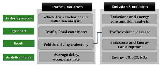
Figure 2. Emission calculation.

The MOVES OpMode method was utilized for microscopic analysis. OpMode is a method for estimating microscopic emissions by classifying second-by-second vehicle trajectory data into 23 operating modes based on velocity, acceleration, and VSP (vehicle-specific power). Since the computational load is extreme when using MOVES Tool to analyze emissions from multiple vehicles, the MOVES-Matrix method can be used as an alternative.

MOVES-Matrix is a model developed by the Georgia Institute of Technology research team. It presents the same results as MOVES but 200 times faster than the MOVES model. For emission calculation, VSP (vehicle-specific power) can be calculated using following formula:

VSP (STP) = (\frac{A}{M}) v + (\frac{B}{M}) \cdot v^{2 +} (\frac{C}{M}) \cdot v^{3} + (\frac{m}{M}) \cdot (a + g \cdot \sin θ) \cdot v

(1)

where A = rolling resistance coefficient (kW∙/m); B = rotational resistance coefficient (kW∙/m²); C = aerodynamic drag coefficient (kW∙3/m³); m = mass of individual test vehicle (metric ton); M = fixed mass factor (metric ton); v = instantaneous vehicle velocity at time t (m/s); a = instantaneous vehicle acceleration (m/s²); g = gravitational acceleration (9.8 m/s²); and u = fractional road grade in percent grade angle (in this study, u = 0).

Year, temperature, humidity, fuel, etc., are required to calculate emissions. For temperature and humidity, 80 F and 70%, i.e., the average values in June in Ansan, were used. The default fuel ratio value of MOVES was used. In summary, the following settings were chosen:

Calendar year, 2021; month, June.
Temperature: 80 F (average temperature in Ansan).
Humidity: 70% (average humidity in Ansan).
Fuel: default for MOVES.

2.3. Calculation of Emissions by Road Sub-Section

The trajectory data extracted from the simulation were processed. In this study, a road segment between two intersections was divided into 25 m sub-sections, and energy consumption and emissions were analyzed. The sub-section length was selected based on the average queue length of 22 m at intersections during off-peak hours. The microscopic emissions in each sub-section were calculated using the MOVES OP mode (Figure 3).

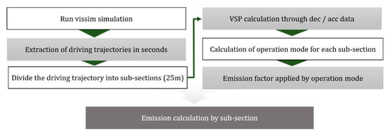
Figure 3. Emissions estimation process.

3. Results

3.1. Analysis of Energy Consumption and Emissions by Sub-Section

In this study, a section of 300 m between intersections was divided into 12 sub-sections of 25 m, and vehicle emissions and energy consumption in each sub-section were calculated (Figure 4). ANOVA was performed to verify the statistical significance of the differences in vehicle emissions and energy consumption by sub-section. Based on the analysis, it was confirmed that energy consumption and emissions were different in the various sub-sections.

Figure 4. Sub-sections (each sub-section is numbered from upstream to downstream).

3.2. Energy Consumption and CO₂

The average and variance of energy consumption and emissions in each sub-section were analyzed. The results are shown in Table 3. It was demonstrated that energy consumption and emission increased significantly in sub-sections that were located immediately before the signal, as shown in Figure 5.

Table 3. Energy and CO₂ by sub-section.

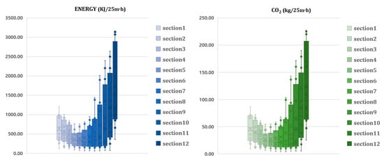
Figure 5. Boxplots of energy and CO₂ by sub-section.

3.3. NOx and CO

The average and variance of NOx and CO emissions in each sub-section are shown in Table 4.

Table 4. NOx and CO by sub-section.

Unlike CO₂, NOx and CO showed the largest emissions in sub-sections where vehicles accelerated. After acceleration, emissions gradually decreased, as shown in Figure 6.

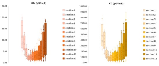
Figure 6. Boxplots of NOx and CO by sub-section.

3.4. Analysis of Variance Results

Analysis of variance was performed to statistically verify that energy consumption and emissions were different in the various sub-sections. Levene’s equal variance test was performed, and the null hypothesis was rejected at a significance level of less than 0.05 (significance probability of 0.00), indicating that equal variance was not assumed (Table 5).

Table 5. Equal variance test results.

Next, robustness testing was performed. The significance probability was less than 0.05, meaning that energy consumption and emissions were statistically different in the various sub-sections, as shown in Table 6.

Table 6. Robustness test results.

3.5. Correlation Analysis of Traffic Flow Characteristics and Emissions by Sub-Section

In this study, the differences in energy consumption and emissions according to the location were derived, and it was confirmed that emissions increased rapidly in specific sections, such as right before and after the signal. Therefore, in order to derive the cause of the variation in emissions by sub-section, the traffic flow characteristics of each sub-section according to the signal were derived, and the correlation between energy consumption and emissions was analyzed. In this study, seven traffic flow characteristics were selected as traffic flow characteristic analysis indicators: average speed (km/h), average acceleration (m/s²), average deceleration (m/s²), occupancy rate (%), average delay (s), speed deviation (km/h), and acceleration deviation (m/s²). In this study, correlations were identified using Pearson’s correlation coefficient and two-tailed test results.

In this study, the correlation between energy consumption and each emission type was analyzed, and the analysis results are shown in Table 7. As a result of the correlation analysis, it was confirmed that the correlation coefficient between energy consumption and CO₂ had a high positive correlation of 1, and the correlation coefficient between NOx and CO had a high positive correlation of 0.91.

Table 7. Results of correlation analysis of energy consumption and emissions.

As a result of the correlation analysis, average speed and average deceleration showed negative correlations with energy consumption and CO₂ emissions, while average acceleration, occupancy rate, average delay, speed deviation, and acceleration noise showed positive correlations.

Three traffic flow characteristics that were highly correlated with energy consumption and CO₂ were average speed (km/h), average delay (s), and occupancy rate (%). Among them, the correlation coefficient of average delay (s) was 0.76, as shown in Table 8, which was the highest positive correlation. It was found that energy consumption and CO₂ generation increased in the sections where the average speed was low, and that delay occurred with a high occupancy rate, as shown in Figure 7.

Table 8. Results of correlation analysis of energy, CO₂, and traffic flow characteristics.

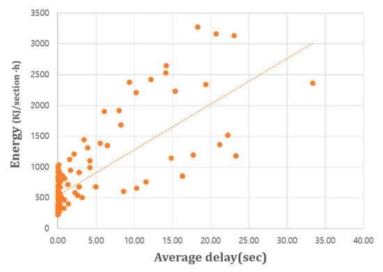
Figure 7. Correlation between energy and average delay.

Two traffic flow characteristics correlated with NOx and CO emissions were average acceleration (m/s²) and average delay (s). Average acceleration (m/s²) showed the highest positive correlation, as shown in Table 9. It was found that the amount of NOx and CO generation increased in the sections where the acceleration of vehicles was high, as shown in Figure 8.

Table 9. Results of correlation analysis of NOx, CO, and traffic flow characteristics.

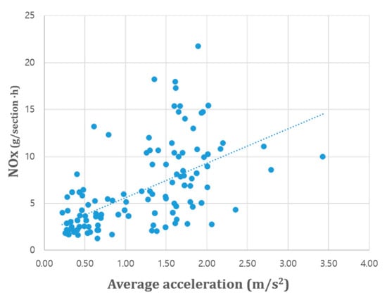
Figure 8. Correlation between NOx and average acceleration.

3.6. Emissions and Energy Consumption Levels by Sub-Section

Cluster analysis was performed to investigate emissions and energy consumption levels by sub-section. The K-means technique was used for cluster analysis. Silhouette analysis was conducted to select the optimal number of clusters, and six clusters were selected; energy consumption and air pollution levels by sub-section were classified into six levels, as shown in Table 10.

Table 10. Cluster analysis results.

Analysis of variance (ANOVA) was performed to verify the statistical significance of cluster analysis. It was found that there were significant differences in both energy consumption and emissions by cluster, as shown in Table 11.

Table 11. Cluster analysis ANOVA results.

The severity of emissions and energy consumption was investigated. Energy consumption and CO₂ showed similar outputs, as they gradually increased in sections closer to the signal. In addition, it was demonstrated that they increased during peak hours, as shown in Table 12 and Table 13. The color of the tables represents the severity of emissions and energy consumption. It can be seen that emissions and energy consumption is higher in downstream locations and peak hours, compared to upstream locations and off-peak hours.

Table 12. Energy consumption.

Table 13. CO₂ generation.

NOx and CO demonstrated similar outputs. They gradually increased in sections closer to the signal, similar to energy consumption and CO₂, as shown in Table 14 and Table 15. However, NOx and CO demonstrated increases in the section immediately after the signal, where vehicles accelerated, unlike energy consumption and CO₂. As expected, NOx and CO were more abundantly generated during peak hours.

Table 14. NOx generation.

Table 15. CO generation.

4. Conclusions and Discussion

In this study, a road segment between two intersections was divided into sub-sections, and energy consumption and emission generation were analyzed. Since there are unique driving behaviors depending on the section of a road segment, energy consumption and emission generation patterns were identified. It was found that there were differences in energy consumption and emission generation in the various sub-sections according to traffic flow characteristics such as speed, delay, and acceleration. In addition, emissions and energy consumption were analyzed using cluster analysis. The findings in this study are expected to provide more detailed and quantitative data for better modeling energy consumption and emissions in urban areas. With the increase in the attention paid to public health, air quality is considered one of the criteria for selecting locations for facilities dedicated to vulnerable users, such as elementary schools and elderly care centers. This paper offers traffic-related air pollution information. However, this study has the following limitations: This analysis only considered passenger vehicles and did not include any truck traffic. However, it is known that emissions from diesel trucks account for a large proportion of road transport pollutants. Therefore, additional analyses, including other vehicle types, would present more accurate outputs. In addition, a section with a speed limit of 50 km/h was set as the analysis range in order to not consider changes in emissions due to changes in the speed limit. However, roads around children’s facilities, which are vulnerable to air pollution, tend to have lower speed limits. Therefore, in future studies, it is necessary to implement various road conditions and analyze the emission patterns that affect respiratory diseases. In addition, in this study, the unit of the sub-section was assumed, considering the average queue length at the intersection to reflect the change in vehicle delay and traffic flow characteristics. However, for more accurate pattern analysis, it is necessary to study the reasonable sub-section criteria that can derive the change in driving behavior at signalized intersections through additional research.

Author Contributions

Methodology, D.K.; Validation, J.K.; Formal analysis, S.J.; Investigation, K.-H.S., S.M.L. and S.E.; Writing – original draft, W.S. All authors have read and agreed to the published version of the manuscript.

Funding

This work was partially supported by NRF-2020R1A2C1011060 and NRF-2022K1A3A1A09078712 Data4Transport – Harnessing Big data to improve intersection traffic operation in urban cities (Korean government).

Institutional Review Board Statement

Not applicable.

Informed Consent Statement

Not applicable.

Data Availability Statement

Data available on request.

Conflicts of Interest

The authors declare no conflict of interest.

References

Joo, S. Development of Integrated Evaluation Methodology for Traffic Management Strategies Considering Public Health and Traffic Safety. Ph.D. Thesis, Hanyang University, Seoul, Republic of Korea, 2017. [Google Scholar]
Park, J.; Jeong, S.; Lim, G. A study on how to reduce exhaust gas emissions using intersection signaling strategies. J. Korean Soc. Transp. Sci. 2005, 48, 357–364. [Google Scholar]
Zhang, Y.; Lv, J.; Wang, W. Evaluation of vehicle acceleration models for emission estimation at an intersection. Transp. Res. Part D Transp. Environ. 2013, 18, 46–50. [Google Scholar] [CrossRef]
Lv, J.; Zhang, Y. Effect of signal coordination on traffic emission. Transp. Res. Part D Transp. Environ. 2012, 17, 149–153. [Google Scholar] [CrossRef]
Lv, J.; Zhang, Y.; Zietsman, J. Investigating emission reduction benefit from intersection signal optimization. J. Intell. Transp. Syst. 2013, 17, 200–209. [Google Scholar] [CrossRef]
Samaras, C.; Tsokolis, D.; Toffolo, S.; Magra, G.; Ntziachristos, L.; Samaras, Z. Enhancing average speed emission models to account for congestion impacts in traffic network link-based simulations. Transp. Res. Part D: Transp. Environ. 2019, 75, 197–210. [Google Scholar] [CrossRef]
Heo, H.; Shin, H.; Kim, J.; Lee, K. A study on microscopic emission factor estimation using GPS vehicle driving trajectory data and MOVES database. J. Korean Road Soc. 2022, 24, 45–54. [Google Scholar]
Boubaker, S.; Rehimi, F.; Kalboussi, A. Impact of intersection type and a vehicular fleet’s hybridization level on energy consumption and emissions. J. Traffic Transp. Eng. (Engl. Ed.) 2016, 3, 253–261. [Google Scholar] [CrossRef]
Han, D.; Lee, Y.; Jang, H. Establishment of a vehicle emission calculation model considering vehicle driving conditions. J. Korean Soc. Transp. 2011, 29, 107–120. [Google Scholar]
Han, D. Development of CO₂ Emission Estimating Methodology of Electronic Toll Collection System Based on Instantaneous Speed and Acceleration. J. Transp. Res. 2012, 19, 63–76. [Google Scholar]
Shancita, I.; Masjuki, H.; Kalam, M.; Fattah, I.; Rashed, M.; Rashedul, H. A review on idling reduction strategies to improve fuel economy and reduce exhaust emissions of transport vehicles. Energy Convers. Manag. 2014, 88, 794–807. [Google Scholar] [CrossRef]
Al-Arkawazi, S. Measuring the influences and impacts of signalized intersection delay reduction on the fuel consumption, operation cost and exhaust emissions. Civ. Eng. J. 2018, 4, 552–571. [Google Scholar] [CrossRef]
Xiaodan, X.; Liu, H.; Anderson, J.; Xu, Y.; Hunter, M.; Rodgers, M.; Guensler, R. Estimating Project-Level Vehicle Emissions with Vissim and MOVES-Matrix. Transp. Res. Rec. J. Transp. Res. Board 2016, 2570, 107–117. [Google Scholar]
Abou-Senna, H. Microscopic Assessment of Transportation Emissions on Limited Access Highways. Ph.D. Thesis, University of Central Florida, Orlando, FL, USA, 2012. [Google Scholar]
Abou-Senna, H.; Radwan, E. VISSIM/MOVES integration to investigate the effect of major key parameters on CO₂ emissions. Transp. Res. Part D Transp. Environ. 2013, 21, 39–46. [Google Scholar] [CrossRef]
Liu, H.; Kim, D. Simulating the uncertain environmental impact of freight truck shifting programs. Atmos. Environ. 2019, 214, 116847. [Google Scholar] [CrossRef]
Meneguzzer, C.; Gastaldi, M.; Rossi, R.; Gecchele, G.; Prati, M. Comparison of exhaust emissions at intersections under traffic signal versus roundabout control using an instrumented vehicle. Transp. Res. Procedia 2017, 25, 1597–1609. [Google Scholar] [CrossRef]
Kim, Y.; Hong, S.; Lee, T.; Park, J. Complementary direction of a model for calculating greenhouse gas emissions in the transportation sector using average vehicle speed. J. Korean Soc. Transp. 2012, 30, 117–126. [Google Scholar] [CrossRef]
Ehsani, M.; Ahmadi, A.; Fadai, D. Modeling of vehicle fuel consumption and carbon dioxide emission in road transport. Renew. Sustain. Energy Rev. 2016, 53, 1638–1648. [Google Scholar] [CrossRef]
Stogios, C.; Kasraian, D.; Roorda, M.; Hatzopoulou, M. Simulating impacts of automated driving behavior and traffic conditions on vehicle emissions. Transp. Res. Part D Transp. Environ. 2019, 76, 176–192. [Google Scholar] [CrossRef]
Shaheen, S.; Bouzaghrane, M. Mobility and energy impacts of shared automated vehicles: A review of recent literature. Curr. Sustain./Renew. Energy Rep. 2019, 6, 193–200. [Google Scholar] [CrossRef]
Zheng, F.; Li, J.; Van Zuylen, H.; Lu, C. Influence of driver characteristics on emissions and fuel consumption. Transp. Res. Procedia 2017, 27, 624–631. [Google Scholar] [CrossRef]
Jang, S.; Wu, S.; Kim, D.; Song, K.-H.; Lee, S.M.; Suh, W. Impact of Lowering Speed Limit on Urban Transportation Network. Appl. Sci. 2022, 12, 5296. [Google Scholar] [CrossRef]
Kim, D.; Ko, J.; Xu, X.; Liu, H.; Rodgers, M.; Guensler, R. Evaluating the Environmental Benefits of Median Bus Lanes: Microscopic Simulation Approach. Transp. Res. Rec. 2019, 2673, 663–673. [Google Scholar] [CrossRef]
Yuan, W.; Frey, H.; Wei, T. Fuel use and emission rates reduction potential for light-duty gasoline vehicle eco-driving. Transp. Res. Part D Transp. Environ. 2022, 109, 103394. [Google Scholar] [CrossRef]
Tang, T.; Yi, Z.; Lin, Q. Effects of signal light on the fuel consumption and emissions under car-following model. Phys. A Stat. Mech. Its Appl. 2017, 469, 200–205. [Google Scholar] [CrossRef]
Pathak, S.; Sood, V.; Singh, Y.; Channiwala, S. Real world vehicle emissions: Their correlation with driving parameters. Transp. Res. Part D Transp. Environ. 2016, 44, 157–176. [Google Scholar] [CrossRef]
Ozguven, E.; Ozbay, K.; Iyer, S. A simplified emissions estimation methodology based on MOVES to estimate vehicle emissions from transportation assignment and simulation models. In Proceedings of the 92nd Annual Meeting of the Transportation Research Board, Washington, DC, USA, 13–17 January 2013. [Google Scholar]
Matsumoto, Y.; Oshima, T.; Iwamoto, R. Effect of information provision around signalized intersection on reduction of CO₂ emission from vehicles. Procedia-Soc. Behav. Sci. 2014, 111, 1015–1024. [Google Scholar] [CrossRef]
Lin, C.; Zhou, X.; Wu, D.; Gong, B. Estimation of emissions at signalized intersections using an improved MOVES model with GPS data. Int. J. Environ. Res. Public Health 2019, 16, 3647. [Google Scholar] [CrossRef] [PubMed]
Deschle, N.; van Ark, E.; van Gijlswijk, R.; Janssen, R. Impact of Signalized Intersections on CO₂ and NOx Emissions of Heavy Duty Vehicles. Energies 2022, 15, 1242. [Google Scholar] [CrossRef]
Kutlimuratov, K.; Khakimov, S.; Mukhitdinov, A.; Samatov, R. Modelling traffic flow emissions at signalized intersection with PTV vissim. In E3S Web of Conferences; EDP Sciences: Paris, France, 2021; Volume 264, p. 02051. [Google Scholar]
Rittger, L.; Schmidt, G.; Maag, C.; Kiesel, A. Driving behaviour at traffic light intersections. Cogn. Technol. Work. 2015, 17, 593–605. [Google Scholar] [CrossRef]
Karabag, H. The Impact of Vehicle Modal Activity and Green Light Optimized Speed Advisory (GLOSA) on Exhaust Emissions through the Integration of VISSIM and MOVES. Ph.D. Thesis, The Florida State University, Tallahassee, FL, USA, 2019. [Google Scholar]

Figure 1. Analysis process.

Figure 2. Emission calculation.

Figure 3. Emissions estimation process.

Figure 4. Sub-sections (each sub-section is numbered from upstream to downstream).

Figure 5. Boxplots of energy and CO₂ by sub-section.

Figure 6. Boxplots of NOx and CO by sub-section.

Figure 7. Correlation between energy and average delay.

Figure 8. Correlation between NOx and average acceleration.

Table 1. Scope of analysis.

Scope of Analysis	Direction
Section	Clothing Town Intersection `→` Ansan Jeil Church Intersection	Ansan Jeil Church Intersection `→` Clothing Town Intersection
	Songho High School Intersection `→` KEPCO Intersection	KEPCO Intersection `→` Songho High School Intersection
	KEPCO Intersection `→` Ansan 5th Bridge Intersection	Ansan 5th Bridge Intersection `→` KEPCO Intersection

Table 2. Traffic flow characteristics.

Variable	Unit	Definition
Average speed	km/h	Average speed of vehicles within sub-section
Average acceleration	m/s²	Average acceleration of vehicles within sub-section
Average deceleration	m/s²	Average deceleration of vehicles within sub-section
Occupancy rate	%	Length of time vehicles stayed in the sub-section
Average delay	S	Average vehicle time delay to pass sub-section
Speed deviation	km/h	Difference in speed between vehicles in the sub-section
Acceleration deviation	m/s²	Acceleration difference between vehicles in the sub-section

Table 3. Energy and CO₂ by sub-section.

Sub-Section		Energy (KJ/Section·h)		CO₂ (Kg/Section·h)
Sub-Section		Average	Variance	Average	Variance
Upstream	Sub-section 1	637	11,590	46	599
`↓`	Sub-section 2	546	8954	39	463
	Sub-section 3	458	62,172	33	321
	Sub-section 4	363	39,856	26	206
	Sub-section 5	366	46,642	26	241
	Sub-section 6	386	61,106	28	315
	Sub-section 7	425	88,734	31	459
	Sub-section 8	545	228,459	39	1180
	Sub-section 9	751	584,323	54	3019
	Sub-section 10	927	793,587	67	4101
	Sub-section 11	1166	775,257	84	4006
Downstream	Sub-section 12	1739	1,097,776	125	5673

Table 4. NOx and CO by sub-section.

Sub-Section		NOx (g/Section·h)		CO (g/Section·h)
Sub-Section		Average	Variance	Average	Variance
Upstream	Sub-section 1	10.5	30.1	466.3	54,804.8
`↓`	Sub-section 2	8.6	13.5	371.8	24,769.6
	Sub-section 3	4.5	4.1	148.2	5076.5
	Sub-section 4	2.5	1.9	79.5	2888.0
	Sub-section 5	2.6	2.6	86.4	3974.7
	Sub-section 6	2.9	3.2	96.9	5713.4
	Sub-section 7	3.0	5.0	106.8	7640.1
	Sub-section 8	3.2	5.9	114.7	7798.9
	Sub-section 9	4.3	12.8	151.8	16,082.8
	Sub-section 10	5.6	26.4	203.6	36,770.7
	Sub-section 11	7.2	41.4	272.3	71,489.6
Downstream	Sub-section 12	10.1	55.1	379.7	92,994.1

Table 5. Equal variance test results.

Homogeneity of Variance Results
	F	df1	df2	P
Energy	11.31	11	132	0.000
CO₂	11.49	11	132	0.000
NOx	8.81	11	132	0.000
CO	6.18	11	51.657	0.000

Table 6. Robustness test results.

Robustness Test Results
	F	df1	df2	P
Energy	3.37	11	51.72	0.001
CO₂	3.35	11	51.72	0.002
NOx	6.18	11	51.65	0.000
CO	7.04	11	51.66	0.000

Table 7. Results of correlation analysis of energy consumption and emissions.

Correlation Analysis Results
	ENERGY	CO₂	NOx	CO
Energy	-	-	-	-
CO₂	1	-	-	-
NOx	0.79	0.79	-	-
CO	0.72	0.72	0.91	-

Table 8. Results of correlation analysis of energy, CO₂, and traffic flow characteristics.

	Average Speed	Average Acc	Average Dec	Occupancy Rate	Average Delay	Speed Deviation	Acc Deviation
Energy CO₂	−0.69	0.58	−0.57	0.61	0.76	0.36	0.36

Table 9. Results of correlation analysis of NOx, CO, and traffic flow characteristics.

	Average Speed	Average Acc	Average Dec	Occupancy Rate	Average Delay	Speed Deviation	Acc Deviation
NOx	−0.41	0.55	−0.22	0.36	0.46	0.22	0.24
CO	−0.36	0.61	−0.14	0.29	0.45	0.08	0.23

Table 10. Cluster analysis results.

	Cluster	N	Average	Variance	Minimum	Maximum
Energy (KL/25 m·h)	1	27	71.9	10,122.1	32.8	99.4
	2	43	171.3	14,621.8	125.1	224.4
	3	29	320.2	41,962.8	242.2	397.2
	4	19	488.4	47,179.7	418.8	573.0
	5	15	770.5	391,088.1	610.1	1066.0
	6	11	1448.2	441,535.6	1224.9	1817.2
CO₂ (Kg/25 m·h)	1	27	5.2	516.3	2.3	7.1
	2	43	12.3	755.6	8.9	16.2
	3	29	23.2	2119.8	17.4	28.6
	4	19	35.1	2437.9	30.1	41.2
	5	15	55.3	20,208.8	43.8	76.6
	6	11	104.1	44,793.2	88.0	130.6
NOx (g/25 m·h)	1	25	0.5	0.03	0.3	0.9
	2	19	1.5	0.15	1.1	2.5
	3	29	2.9	0.17	2.6	3.9
	4	35	5.5	0.93	4.2	7.2
	5	23	9.8	1.6	7.8	11.4
	6	13	15.8	3.5	12.7	18.8
CO (g/25 m·h)	1	35	2.9	2.3	6.6	52.1
	2	33	7.6	3.1	54.2	106.8
	3	30	15.9	10.1	113.3	218.2
	4	20	29.8	10.3	231.8	345.1
	5	9	42.2	21.3	376.1	481.3
	6	17	67.1	145.2	482.6	885.0

Table 11. Cluster analysis ANOVA results.

ANOVA
	Cluster		Error		F	Sig.
	Mean Square	Df	Mean Square	df	F	Sig.
Energy	12,702,064	5	3,063,407.3	138	571.857	0.000
CO₂	65,594,661	5	15,826.116	138	571.953	0.000
NOx	647.05244	5	180.99542	138	493.345	0.000
CO	114,956.91	5	33.565867	138	472.621	0.000

Table 12. Energy consumption.

		Upstream				→				Downstream				Stdev
Time		1	2	3	4	5	6	7	8	9	10	11	12	Stdev
Peak hours	(1)													797
	(2)													535
	(3)													824
	(4)													900
	(5)													263
	(6)													237
Off-peak hours	(1)													265
	(2)													185
	(3)													386
	(4)													579
	(5)													151
	(6)													83

Table 13. CO₂ generation.

		Upstream				→				Downstream				Stdev
Time		1	2	3	4	5	6	7	8	9	10	11	12	Stdev
Peak hours	(1)													54
	(2)													38
	(3)													59
	(4)													65
	(5)													19
	(6)													17
Off-peak hours	(1)													19
	(2)													13
	(3)													27
	(4)													42
	(5)													11
	(6)													6

Table 14. NOx generation.

		Upstream				→				Downstream				Stdev
Time		1	2	3	4	5	6	7	8	9	10	11	12	Stdev
Peak hours	(1)													5.9
	(2)													4.4
	(3)													6.0
	(4)													5.4
	(5)													2.5
	(6)													1.7
Off-peak hours	(1)													2.5
	(2)													2.3
	(3)													3.1
	(4)													3.5
	(5)													1.4
	(6)													0.8

Table 15. CO generation.

		Upstream								Downstream				Stdev
Time		1	2	3	4	5	6	7	8	9	10	11	12	Stdev
Peak hours	(1)													247.1
	(2)													189.3
	(3)													263.1
	(4)													245.2
	(5)													97.9
	(6)													98.9
Off-peak hours	(1)													113.9
	(2)													107.2
	(3)													119.5
	(4)													139.9
	(5)													66.9
	(6)													51.2

Disclaimer/Publisher’s Note: The statements, opinions and data contained in all publications are solely those of the individual author(s) and contributor(s) and not of MDPI and/or the editor(s). MDPI and/or the editor(s) disclaim responsibility for any injury to people or property resulting from any ideas, methods, instructions or products referred to in the content.

© 2023 by the authors. Licensee MDPI, Basel, Switzerland. This article is an open access article distributed under the terms and conditions of the Creative Commons Attribution (CC BY) license (https://creativecommons.org/licenses/by/4.0/).

Road-Section-Based Analysis of Vehicle Emissions and Energy Consumption

Abstract

1. Introduction