Numerical Investigation of Recommended Operating Parameters Considering Movement of Polymetallic Nodule Particles during Hydraulic Lifting of Deep-Sea Mining Pipeline

Abstract

Previously conducted studies have established that pipeline hydraulic transport systems are currently the most promising deep-sea mining systems, and the pipeline transport performance of polymetallic nodules is one of the technical priorities. In this paper, a coupled CFD–DEM approach is adopted to numerically calculate the solid–liquid two-phase flow of seawater with polymetallic nodules. Small-scale experiments were conducted to validate the coupled model. Particle dynamics analysis was carried out under different inlet flow rates, feed concentrations and nodule fragmentation levels. The simulation results show that different operating parameters have significant effects on the pipeline transportation process. With low inlet flow rate, high feed concentration, and high percentage of large particles, the particle distribution and motion characteristics show a trend that is not conducive to safe transport. A set of recommended operating parameters for hydraulic transport of polymetallic nodule pipelines was summarized.

1. Introduction

One key technology of deep ocean mining is transporting the collected minerals from a depth of several thousand meters [1]. Vertical pipeline hydraulic lifting is the most practical and potential deep-sea ore transportation method widely recognized internationally [2]. The pipe flow based on the hydraulic lifting method is a two-phase flow [3]. Due to the heterogeneity and discontinuity of the ore in the transportation process, if the appropriate transportation conditions cannot be selected, the local concentration of the ore in the pipeline increases to form a slug flow or even blockage [4]. Therefore, to improve safety and efficiency, it is of great significance to study the dynamic characteristics of the solid–liquid two-phase flow and the movement characteristics of ore particles in the vertical pipeline.

Early research on hydraulic transportation mainly focused on the suspended flow of small particle size solid materials in water. Based on physical experiments, empirical formulas for calculating various transportation parameters were obtained [5,6]. Many studies on the use of physical model test methods for hydraulic transportation have been carried out. The scale test method was employed to investigate the effect of particle shape and size on pressure loss [7]. A comparative experimental study of natural and artificial manganese nodules in hoses was carried out to explore their effects on flow rate, particle size, hose shape, and other parameters [8,9]. It was also found that the pressure loss due to friction of solid–liquid two-phase flow in the hydraulic conveying process is positively correlated with the pipe inclination, and the increase of flow rate can mitigate the effect of pipe inclination on pressure loss [10]. For the transportability of rigid mixtures, there have been studies analyzing the effect of activation treatments on individual components or on the whole mixture [11]. High-speed cameras and radioisotope tracking methods are widely used in measuring the motion state and slip speed of particles in hydraulic lifting pipelines [12].

In an actual engineering system, the deep-sea mining pipeline system is a vast and complex integrated system [13], laboratory physics experiments do not adequately represent the actual situation. In contrast to physical experiments, the studies of particle motion characteristics in pipeline using theoretical analysis and numerical simulation methods were gradually developed. A theoretical model of solid–liquid two-phase flow in a vertical pipeline was presented based on the conservation of momentum equation, D’Alembert’s principle, and the continuity equation [14]. Analytical mathematical modeling was used to investigate how to reduce the energy cost of solid–liquid mixtures during transport [15]. By using physical modeling on a simulation model, the transport performance of the created composite material was studied while maintaining the specified strength properties. Based on this model, it was also concluded that the water–solid ratio has a significant effect on the transport length and the change of properties during transportation [16]. A mathematical model for the prediction of pressure loss of flexible slant pipeline was established and verified by hydraulic transportation test [17]. Based on the concepts of internal friction angle and friction coefficient between different materials, a theoretical model for calculating the friction force between particles and pipe wall was established [18]. Using a combination of theoretical analysis and experimental verification, a semi-theoretical and semi-empirical formula for calculating the shear stress of the pipe wall under blockage conditions was established [19,20]. A numerical solver was developed for marine ore transportation based on the Lagrange method for the flow assurance problem of deep-sea mining [21]. Based on the finite element analysis method, a deep-sea transportation pipeline model was established, and the force and motion laws under the combined effects of the outflow of the ocean, the internal two-phase flow, and the drag of the mining vessel were explored [22]. FLUENT software is used to simulate and calculate the operation process of lift pumps and flexible hoses [23]. The CFD method was adopted to simulate the pipeline movement in the marine operating environment and analyzed the impact of the dynamic marine environment on the two-phase flow field [24].

However, the ore particles are large, dense, and have poor followability in seawater [25]. The conventional computational fluid dynamics method is not suitable for studying the uneven solid–liquid two-phase flow. The particle discrete element method (DEM) [26] treats particles as discrete entities, considering the particle structure and collisions, and can fully obtain the dynamic information of the particles. The coupling of DEM and CFD methods can solve the solid–liquid two-phase flow problem more accurately and efficiently. CFD–DEM has already exerted its unique advantages in researching two-phase flow in many other machinery and equipment [27,28]. In the field of deep-sea mining transportation systems, Huang et al. [29] used the CFD–DEM method to analyze the transient state of the solid–liquid two-phase flow in the centrifugal pump. Chen et al. [30] used the CFD–DEM method to analyze the slurry flow in hydraulic pipelines with different particle shapes and explored the clogging conditions. The CFD–DEM method was also applied to the numerical simulation of horizontal pipeline hydraulic conveying process to study the variation law of pipeline dynamic parameters under different particles and pipeline parameters [31].

The transport performance of polymetallic nodule particles in a pipeline hydraulic system is one of the important technical issues in deep-sea mining systems. Analyzing the above, it can be noted that the application of the coupled CFD–DEM numerical simulation method is a popular and effective way to perform two-phase flow analysis. Therefore, the purpose of this study is to analyze the effect of different operating parameters on the polymetallic nodule pipeline transport process using the CFD–DEM method. To achieve this goal, the following tasks need to be solved: (1) analysis of kinetic principles of solid–liquid two-phase flow, formation of coupled CFD–DEM method and establishment of simulation model; (2) performing hydraulic transport simulation calculations and analysis of particle motion and distribution; (3) analysis of influencing factors and proposal of optimized operating parameters.

2. Principles and Methods

The two-phase flow in a deep-sea hydraulic pipeline is very complicated under ore particles’ interaction, seawater, and pipe wall. The related theories of fluid mechanics and solid–liquid two-phase flow are introduced, and physical simulation models are established based on actual engineering parameters to explore the hydraulic pipeline system’s flow phenomenon comprehensively.

2.1. Governing Equation

Seawater is regarded as a continuous field and particles are considered to be discrete items. Navier–Stokes (N–S) equations are the basic equations describing fluid motion, including mass, momentum, and energy conservation equations. In the momentum equation, a disturbance term is introduced to the fluid due to the existence of particles. The fluid control equation is as follows:

$$\frac{\partial \left(\epsilon \rho \right)}{\partial t}+\nabla ·\left(\epsilon \rho u_f\right)=0$$

(1)

$$\frac{\partial \left(\epsilon \rho u_f\right)}{\partial t}+\nabla ·\left(\epsilon \rho u_f{u}_f\right)=-\nabla p+\nabla ·\left(v\epsilon \nabla u_f\right)-\epsilon \rho g+f_{sf}$$

(2)

where $\epsilon$ is the fluid volume fraction; $\rho$ is the fluid density; $t$ is the time; $u_f$ is the fluid velocity; $p$ is the pressure; $v$ is the kinematic viscosity; $g$ is the gravity; $f_{sf}$ represents the momentum exchange between the particle and the fluid [32].

The governing equations of the particle are the momentum conservation equation and the angular momentum conservation equation of the particle.

$$m_s\frac{d{V}_s}{dt}=m_{s}g+F_d+F_p+F_l+F_{am}+F_B+F_c$$

(3)

$$I_s\frac{d{\omega }_s}{dt}=M_{fs}+M_c$$

(4)

where $m_s$ is the particle mass; $V_s$ is the particle velocity; $F_d$ is the fluid resistance; $F_p$ is the pressure gradient force; $F_l$ is the lift force including Magnus force and Saffman force; $F_{am}$ is the additional mass force; $F_B$ is the Basset force; $F_c$ is the contact force between other particles; $I_s$ is the particle moment of inertia; ${\omega }_s$ is the particle angular velocity; $M_{fs}$ is the drag torque of the fluid on the particle; $M_c$ is the contact torque of other particles [33,34].

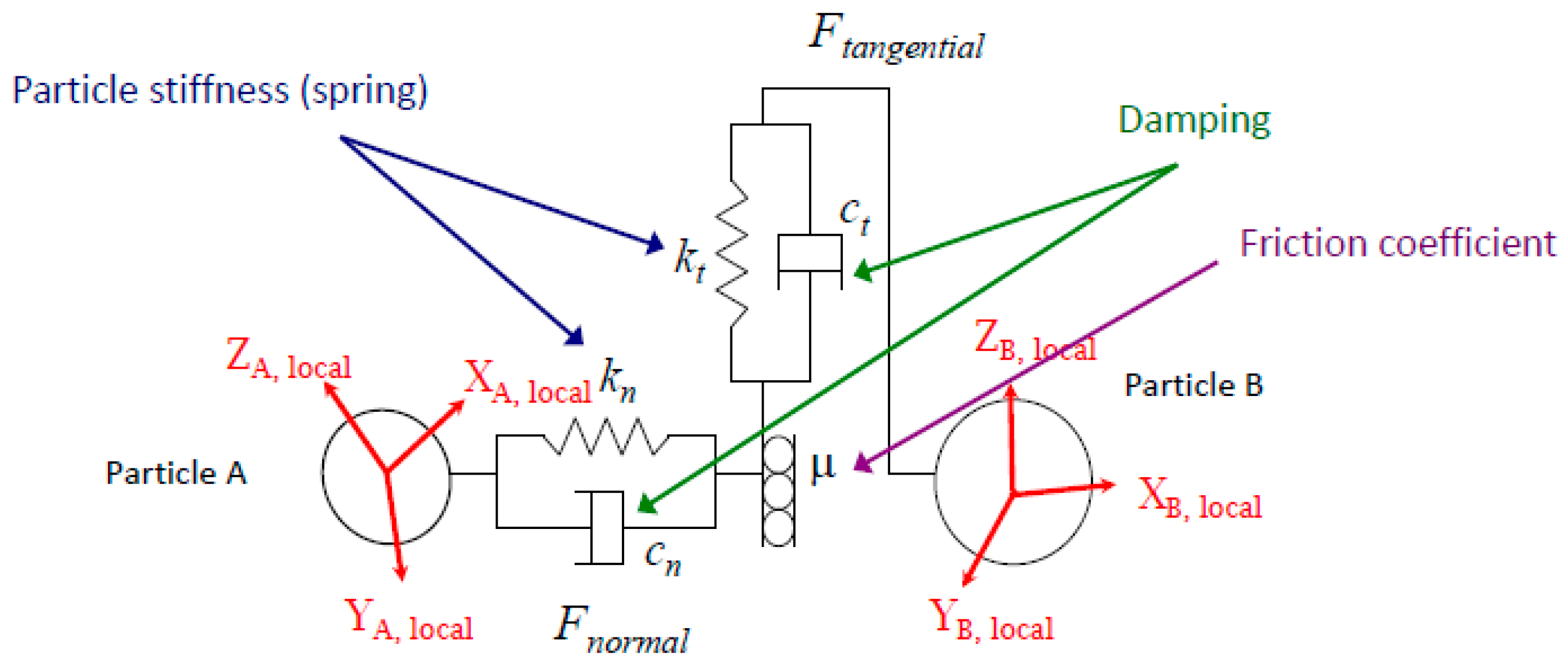
2.2. Particle Contact Model

During the transportation of nodule particles, due to the turbulence effect of the fluid and the changes in the shape of the pipeline, collisions will inevitably occur, and there must be an interaction between particles. In the study of seawater–ore two-phase flow, the Hertz–Mindlin model is widely used to express the contact force and damping force between particles [26,35,36]. The manganese nodules studied in this paper are relatively difficult to degrade, so the Hertz–Mindlin model is adopted. The schematic diagram of the model is shown in Figure 1.

The formulas for calculating the contact between particles A and B are as follows.

$$F_n=-\frac{4}{3}{E}_{eq}{R}_{eq}^{\frac{1}{2}}{\delta }_n{}^{\frac{3}{2}}$$

(5)

$$F_t=-8G_{eq}{\delta }_t\sqrt{R_{eq}{\delta }_n}$$

(6)

$$\frac{1}{E_{eq}}=\frac{1-{\nu }_A^2}{E_A}+\frac{1-{\nu }_B^2}{E_B}$$

(7)

$$\frac{1}{R_{eq}}=\frac{1}{R_A}+\frac{1}{R_B}$$

(8)

where $F_n$ and $F_t$ are the normal contact force and tangential contact force; $E_{eq}$ is the equivalent Young’s modulus, $E_A$ and $E_B$ are the Young’s modulus of particles A and B; $R_{eq}$ is the equivalent contact radius, $R_A$ and $R_B$ are the contact radius of particles A and B; ${\delta }_n$ and ${\delta }_t$ are the normal overlap and tangential overlap; ${\nu }_A$ and ${\nu }_B$ are the Poisson’s ratio of particles A and B; $G_{eq}$ is the equivalent shear modulus.

The formulas for calculating the damping force between particles A and B are as follows.

$$F_{d,n}=-2\sqrt{\frac{5}{3}}\frac{lne}{\sqrt{{ln}^{2}e+{\pi }^2}}\sqrt{E_{eq}{m}_{eq}{(R_{eq}{\delta }_n)}^{\frac{1}{2}}}{v}_n^{rel}$$

(9)

$$F_{d,t}=-2\sqrt{\frac{5}{6}}\frac{lne}{\sqrt{{ln}^{2}e+{\pi }^2}}\sqrt{8G_{eq}{m}_{eq}{(R_{eq}{\delta }_n)}^{\frac{1}{2}}}{v}_t^{rel}$$

(10)

$$\frac{1}{m_{eq}}=\frac{1}{m_A}+\frac{1}{m_B}$$

(11)

where $F_{d,n}$ and $F_{d,t}$ are the normal damping force and tangential damping force; $v_n^{\mathrm{rel}}$ and $v_t^{\mathrm{rel}}$ are the normal component and tangential component of the relative velocity; $m_{eq}$ is the equivalent mass.

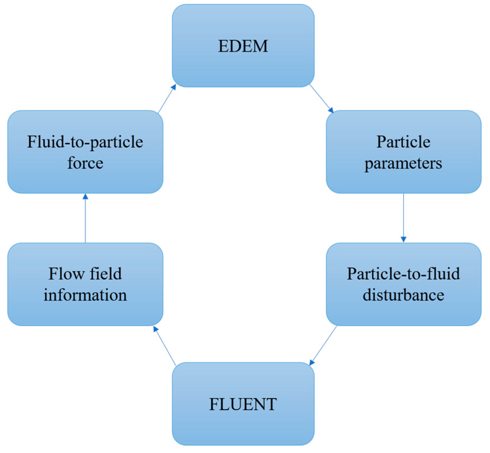
2.3. CFD–DEM Coupling Method

In the CFD–DEM coupling process, the flow and particles are processed using FLUENT and EDEM, respectively. The EDEM–FLUENT coupling process is a transient two-way data transfer process. In the coupling process, the continuous phase flow mode is affected by the discrete phase (and vice versa), and the two software alternately calculate the continuous phase and discrete phase equations until a convergent coupling solution is achieved. First, obtain the flow field information calculated in the previous step and obtain the particles’ force and motion parameters using the calculation models, contact force models, and solving the particle motion differential equations. According to the fluid force received by the particle, the reaction force of the particle on the fluid is obtained, which is used as the source term in the fluid governing equation; by solving the control equations, the flow field information such as pressure and velocity are obtained; the obtained flow field information is used as the input parameter in the next iteration step, and the above process is repeated; through several iterations, the convergence of the flow field and particle motion results is finally achieved, and the calculation of the time step is completed. The dynamic characteristics of the two-phase flow are obtained by repeatedly completing the analysis of multiple time steps. Figure 2 shows the CFD–DEM coupling principle.

To ensure the accuracy of the simulation, the time step is required to meet the accuracy requirements of the simulation results. For EDEM, there is a strong correlation between time step and simulation accuracy. In the case of a small time step, the calculation has excellent accuracy but requires a lot of time. If the time step is too large, particles can behave erratically. This seriously affects the stability of the simulation calculation, and an ‘explosion’ of incorrectly moving elements may occur. The important parameter used to evaluate the time step in EDEM is the Rayleigh time step. The particle time step generally falls in the range of 10⁻⁷ to 10⁻⁴ s [38]. For the FLUENT model, it is necessary to balance the calculation stability and efficiency according to the fluid model and choose a reasonable time step. In practice, the fluid time step falls in the range of 10⁻⁵ to 10⁻² s based on this condition. To ensure the stability of the solution and prevent lagged integration of equations of motion of phases, the time step in FLUENT is an integer multiple of the time step in EDEM [38].

The coupling method calculates the flow field information for a time step in FLUENT and then iterates the same time length in EDEM. The calculation formula of the Rayleigh time step is as follows.

$$T_R=\frac{\pi R}{0.163v+0.877}\sqrt{\frac{\rho }{G}}$$

(12)

where $G$ is the shear modulus of the particle, $v$ is the Poisson’s ratio, $R$ and $\rho$ is the radius and density of the particle.

3. Materials and Models

3.1. Physical Model

Based on laboratory artificial nodules, the density of the simulated polymetallic nodules was set to 2000 kg/m³. The Poisson’s ratio was set to 0.13. The modulus of elasticity as set to 11.5 Gpa. The actual shape of manganese nodules tends to be spherical, and the degradation of the fluid smooths out the edges and corners. Therefore, one single-sphere model was used. The deep-sea polymetallic nodules collected by the mining system are generally large and need to be crushed before entering the pipeline transportation system. Crushing nodules too finely increases the energy cost of the crushing operation and may cause wear and tear on the equipment. However, oversized nodules increase the risk of pipe blockage. To ensure sufficient economic benefits and the safety of the conveying system, the degree of crushing should be moderate, and the particle size should be controlled within 5–30 mm. Three typical particle sizes were adopted for simulation, which were 8 mm, 16 mm, and 24 mm.

The transport pipeline model needs to be long enough to ensure that the two-phase flow can reach a steady state in the pipeline. To ensure both simulation accuracy and less computation time, the length of the pipeline model was set to 3.5 m, and the diameter was set to 195 mm. The pipe material density was 7800 kg/m³, and the shear modulus was set to 41 Gpa. ICEM was used to mesh the transmission pipeline model. Since the pipe was a cylinder with a regular structure, a structured grid was used to improve calculation efficiency [39]. Inflation options were carried out near the pipe wall to better capture the flow near the wall. There were 278,113 nodes and 147,102 elements in the divided grid. To simulate seawater, the density of the fluid in the pipeline was set to 1025 kg/m³.

3.2. Software Settings

In EDEM, the interaction parameters of the Hertz–Mindlin no-slip model are shown in

Table 1. Material interaction parameters.

Materials	Coefficient of Restitution	Coefficient of Static Friction	Coefficient of Rolling Friction
Particle–Particle	0.45	0.28	0.01
Particle–Pipeline	0.48	0.10	0.01

. The time integration method was the Euler method. The Rayleigh time step was automatically calculated as 1.0203 × 10⁻⁵ s according to the parameters such as the radius and density of the particles. To ensure the accuracy and stability of the calculation, the fixed time step was set to 2 × 10⁻⁶ s. In the EDEM settings interface, the estimate cell size option provides guidance on the optimal cell size for a specific simulation time step. The optimal cell size was calculated to be 3.5 times the minimum particle radius, which was 0.014 m.

In FLUENT, the transient calculation and pressure-based solver were selected based on the simulation conditions of the solid–liquid two-phase flow. The Eulerian model was chosen for the multiphase flow model. Regarding the solution of turbulence, the Reynolds Average Navier–Stokes Model (RANS) is widely used. The standard k-epsilon model was adopted. Due to the effect of the particles, the local velocity and pressure of the solid–liquid two-phase flow changed rapidly. In this case, the commonly used standard wall function was not applicable. Therefore, the nonequilibrium wall function was adopted. The inlet was set as a velocity inlet, and the outlet was set as a pressure outlet. The inlet was set at the position of z = 0, and the liquid flow direction was the positive direction of the z-axis. The turbulent intensity and hydraulic diameter were set to 5% and 0.195 m, respectively. According to the time step in EDEM, the length of the time step was set to 1 × 10⁻⁴ s. The total simulation time was set to 6 s to ensure that the particle movement reached a stable state. The direction of gravity was downward along the z-axis.

3.3. Target Variables and Calculation Conditions

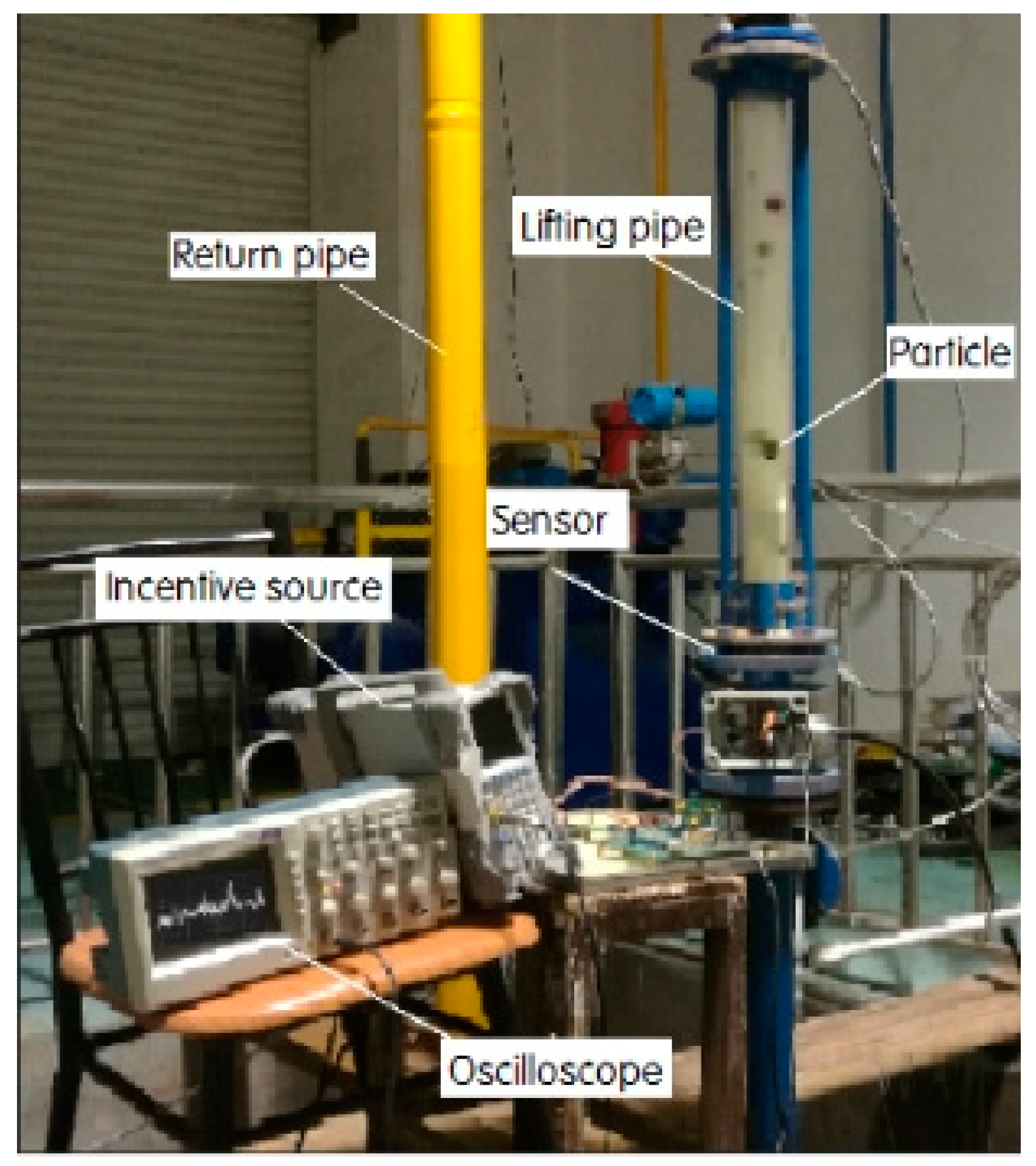
After the large-size polymetallic nodules were collected by the collector head, they were crushed inside the mining robot and the particle size was uniformly reduced to facilitate the subsequent transport process. In a real deep-sea mining system, the degree of polymetallic nodule fragmentation inside the collector cannot be precisely controlled, and the particle size distribution fluctuates. To investigate the effect of different levels of nodule fragmentation on the flow in the vertical pipe and the transport of nodules, four different particle size distributions were set in the numerical simulation. Since it is not possible to treat all nodules to the same particle size at any degree of fragmentation, the specific settings are shown in

Table 2. Particle size distribution settings in the simulation.

Types of Distribution	Percentage of 8 mm Particles	Percentage of 16 mm Particles	Percentage of 24 mm Particles
Even	33.33%	33.33%	33.33%
Small	80%	10%	10%
Medium	10%	80%	10%
Large	10%	10%	80%

.

The conveying fluid speed and the initial feed concentration have a direct influence on the particle conveying efficiency, which are the basic operating parameters of the pipeline hydraulic lifting system. In this simulation, the inlet flow velocity was set to 2 m/s, 3 m/s, 4 m/s, and 5 m/s, and the initial particle volume concentration was set to 6%, 9%, and 12% under the even distribution condition of particles of different sizes. The transportation process simulations under different particle size distributions were carried out, which were performed with an inlet fluid of 3 m/s and an initial particle volume concentration of 9%.

3.4. Validation

This paper is based on a self-developed hydraulic lifting test device to simulate the hydraulic lifting process of ore particles in a vertical pipeline. The hydraulic lifting pipeline experiment system was driven by an impurity pump and speed-regulating motor. A high-speed acquisition camera was used to acquire high-speed images of particle movement in the pipeline. A riser with a pipe diameter of 50 mm and a pipe length of 11 m was used. There was a section of a transparent glass tube in the middle of the riser to observe and collect data. A reflux pipe was set to ensure the reflux circulation of the system. Figure 3 shows the actual photo of the experimental pipeline system. In the published papers, the accuracy of the numerical model regarding the particle distribution was verified using this test system [34]. The relevant comparative validation was carried out for the particle motion trajectory, which is of additional interest in this paper.

The processing method of particle trajectory tracking is to select a target particle in a certain frame of the image, and then, pressing the play button, the selected target point moves with the movement of the particle. After repeating this process, the particle trajectory is recorded, and the particle velocity is calculated. The tracking situation is shown in Figure 4. In the process of particle tracking, the tracking point is jittered, and the trajectory curve is smoothed in postprocessing.

Based on this method, the trajectories of particles at different lifting speeds were obtained. The initial flow velocity was set to 1.14 m/s and 1.25 m/s, respectively. Simulation of the multiphase flow coupled hydraulic transport process was carried out based on the numerical model of this paper with the same parameter settings. The simulated particle motion trajectories were obtained and compared with those in the experiment in Figure 5. The particle trajectories of the experiment and simulation are shown on the left and right sides, respectively. As shown in Figure 5, when the flow rate is low, the collected particle trajectories have greater jitter and overall lateral movement. The particle trajectories in the experiment have the same characteristics as those in the numerical simulation, which illustrates the accuracy of the numerical model.

4. Analysis of Particle Distribution

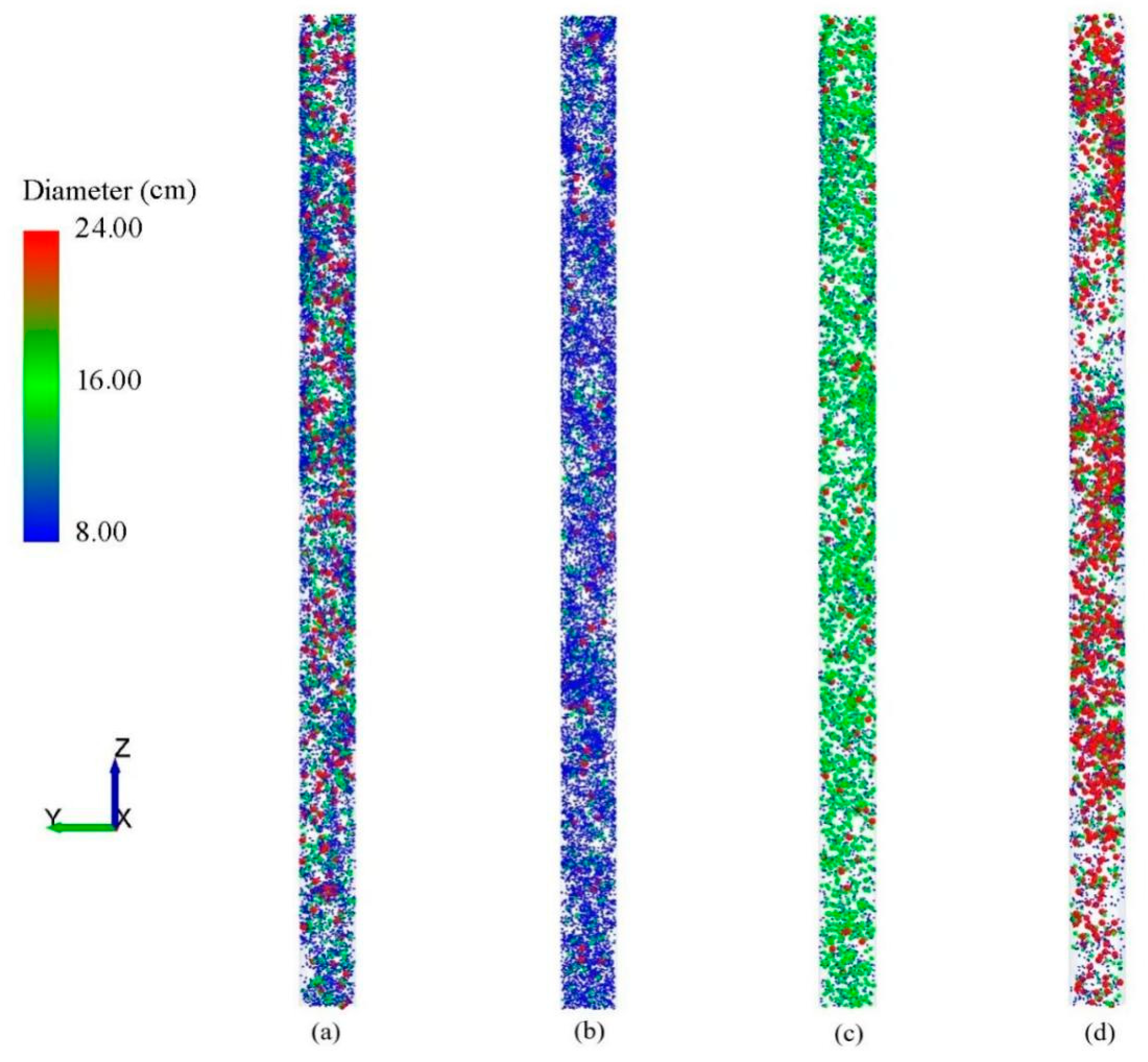
4.1. Overall Distribution

When the inlet flow rate is low, the particles are not uniformly distributed in the pipe. The local concentration of particles near the outlet is large, and there is a slight particle aggregation phenomenon. This aggregation phenomenon occurs mainly because the density of the ore particles is greater than the density of seawater and discontinuous in the two-phase flow, the fluid action of the particles lifting movement relative to the fluid itself movement has a certain hysteresis phenomenon, indicating the existence of relative velocity of particles and fluid. This phenomenon is an unfavorable factor in the process of hydraulic lifting pipeline conveying. As the inlet concentration increases, the risk of further particle accumulation into clumps increases.

As the inlet flow rate increases, the distribution of particles in the pipeline becomes more uniform, and there is almost no local concentration bias and particle aggregation, and the hydraulic lifting process of polymetallic nodules is more stable currently. This is because more frequent momentum and energy exchange occurs between the fluid and the particles at higher flow velocities, which has a more obvious effect on the lifting motion of the particles, and the relative velocity between the particles and the fluid decreases, which eventually makes the hysteresis phenomenon of the particles disappear gradually, thus eliminating particle aggregation. At the same time, the local concentration of particles and the reduction of the frequency of uneven particle motion reduces the kinetic energy lost due to collisions, further improving the following performance of particles and fluid for lifting motion.

After the particle motion in the pipe reaches the steady state, the instantaneous overall particle concentration in the pipe is obtained for different inlet flow rates and feed concentrations at a certain time point, as shown in Figure 6. When the inlet flow rate is 2 m/s, the overall particle concentration in the pipe is significantly larger than the set initial feed concentration. This phenomenon is consistent with the hysteresis effect described above. Particles lift a certain slip velocity relative to the fluid, and the number of particles leaving the calculation domain from the outlet to complete the conveying process is less than the number of particles entering the flow field, resulting in an increase in the overall particle concentration. The degree of particle buildup is greater at high inlet concentrations. As the inlet flow velocity increases, the effect on the lifting motion is more obvious and the overall concentration of particles gradually decreases. Under high inlet flow rate conditions, the instantaneous overall particle concentration in the pipeline even appears to be slightly lower than the feed concentration.

Figure 7 shows the particle distribution in the pipeline under different particle size distribution conditions when the initial flow rate is 3 m/s, and the particle feed concentration is 9%. When there are more particles with a particle size of 8 mm and 16 mm, the particle distribution in the pipeline is more uniform. However, when there are more particles with a particle size of 24 mm, the particle distribution has obvious aggregation and stratification, and the risk of pipeline blockage is higher. The flow with a smaller overall particle size is more stable. The reason for this phenomenon may be that when the weight is not large, the particles are more likely to be driven by the rising fluid during the hydraulic lifting process, and the motion of the particles is more consistent with the fluid motion. Larger particles cause greater disturbance to the fluid. Some large particles that are close together cannot fully receive the lifting force of the fluid, which intensifies the aggregation of particles.

4.2. Local Concentration

The local concentration is an important indicator of whether the polymetallic nodules are in a homogeneous distribution during the lifting process in the pipeline. The local concentration data was acquired at the position of the pipeline with a height of 2 m. Figure 8 shows the local volume concentration of particles when the simulation time is between 2–4 s under different working conditions. When the initial flow velocity is 2 m/s, the local concentration of particles in the pipeline changes quickly and with a relatively large amplitude. This situation is more obvious when the particle concentration is high. The local concentration is an important indicator of whether the polymetallic nodules are in a homogeneous distribution during the lifting process in the pipeline. When the initial concentrations are 6% and 12%, the difference between the upper and lower peak local concentrations exceeds 6.2% and 7.8%, and the highest values are close to 10.3% and 17%, respectively. The reason for this phenomenon is the hysteresis effect of particles under the action of lower-density seawater. When such a staged local concentration is too high, the collision between particles and particles and between particles and pipe walls is significantly enhanced. If the subsequent treatment is not appropriate, it is extremely unfavorable for saving energy consumption for transportation and maintaining the safety of the pipeline system. When the initial flow velocity rises to 4 m/s, the pulsation and increase in the local concentration of particles are alleviated. At higher flow rates, the sliding velocity of particles relative to the fluid is smaller, so the retention effect is no longer noticeable. The reduction of local concentration reduces the risk of blockage in the pipeline to a certain extent.

Figure 9 shows the local concentration variation at the height of 2 m of the pipeline with different particle size distributions within 2–4 s of simulation time. Different particle size distributions have local concentration fluctuations. With the increase in large-size particles, the pulsation of local concentration becomes more severe. In Figure 9d, the upper and lower peaks of the local concentration of particles are close to 3% versus 16%, which corresponds to the stratification phenomenon of particle aggregation in Figure 7d. The solid–liquid two-phase flow in the pipe is not uniform. Smaller particles follow the fluid better than larger particles, and the stagnation phenomenon is not obvious. The risk of clogging increases steeply if the local concentration reaches the highest values shown in the figure. Therefore, polymetallic nodules should be crushed to a particle size no larger than 16 mm before entering the transport pipeline.

4.3. Radial Distribution

Figure 10 shows the radial distribution of concentration in the pipeline under different working conditions. The particles are not uniformly distributed along the radial direction in the pipe. The concentration gradually increases from the center of the pipeline. The particle concentration is highest near r/R = 0.7–0.8, and there is a phenomenon of particle aggregation. The particle concentration near the tube wall is the lowest. This trend is usually the same, and the radial distribution of particles is more uniform under conditions of low flow velocity and low concentration. Since the center fluid velocity is higher, the particles tend to approach and stay on the pipe wall. The fluid in the pipeline has a large flow velocity gradient in the near-wall area, and the particles are subjected to the shear stress of the fluid near the pipe wall to generate a shear moment and rotate. Due to the rotation of the particles, the obvious Magnus force causes the particles to move away from the wall of the tube, reducing the particle concentration in the area near the wall.

Figure 11 shows the radial concentration distribution of different particle size distributions under the conditions of V₀ = 3 m/s and C_v = 9%. The overall radial concentration pattern of various particle size distribution cases is consistent with that of uniform particle size distribution. When there are more large particles, the fluctuation of radial concentration distribution is more dramatic. The possible reason is that the particle aggregation phenomenon is more obvious when there are more large particles, and there are more frequent collisions between particles and more clusters of particles, which affects the distribution of particles along the radial direction.

5. Analysis of Particle Motion

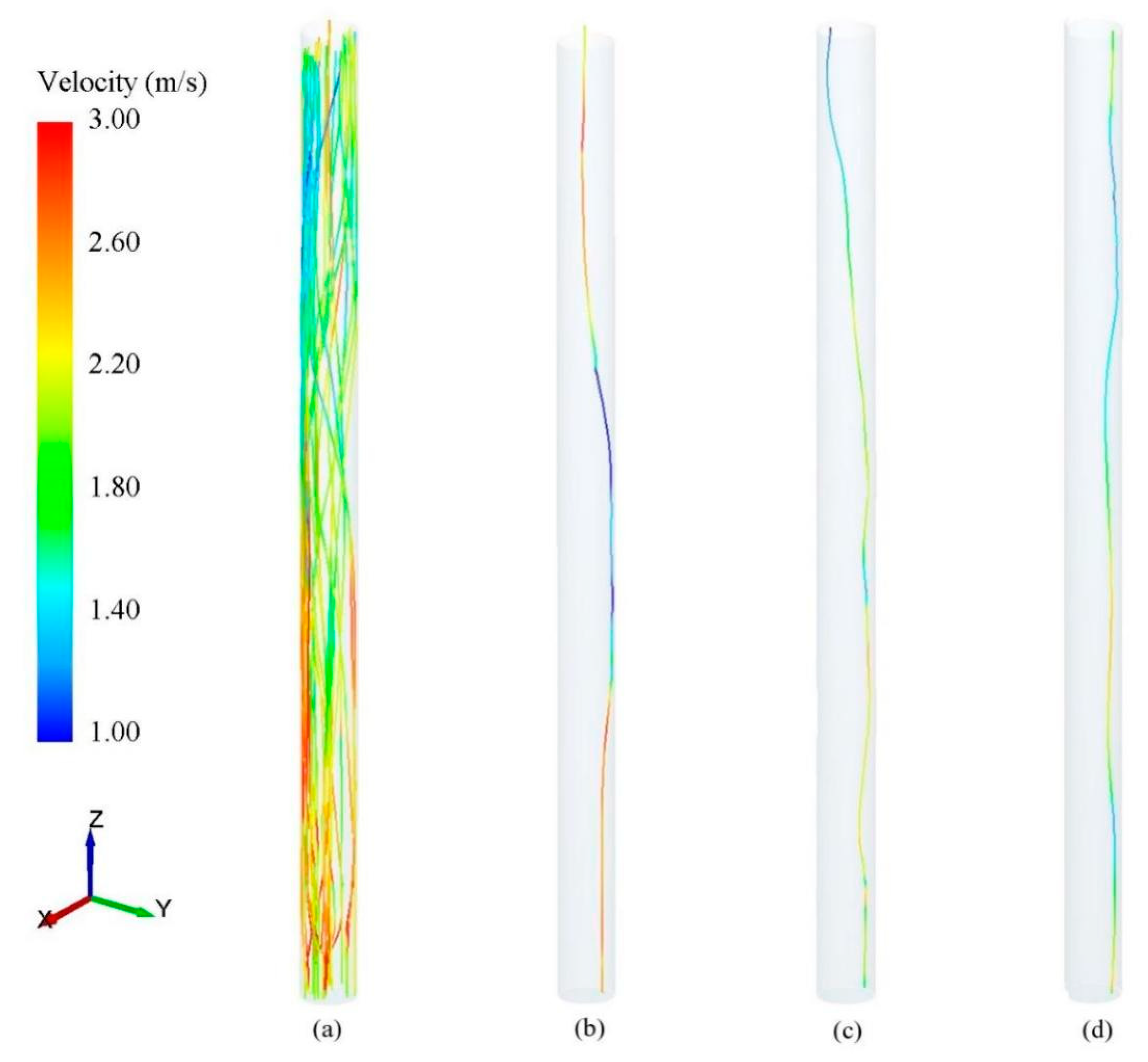
5.1. Movement Trajectory

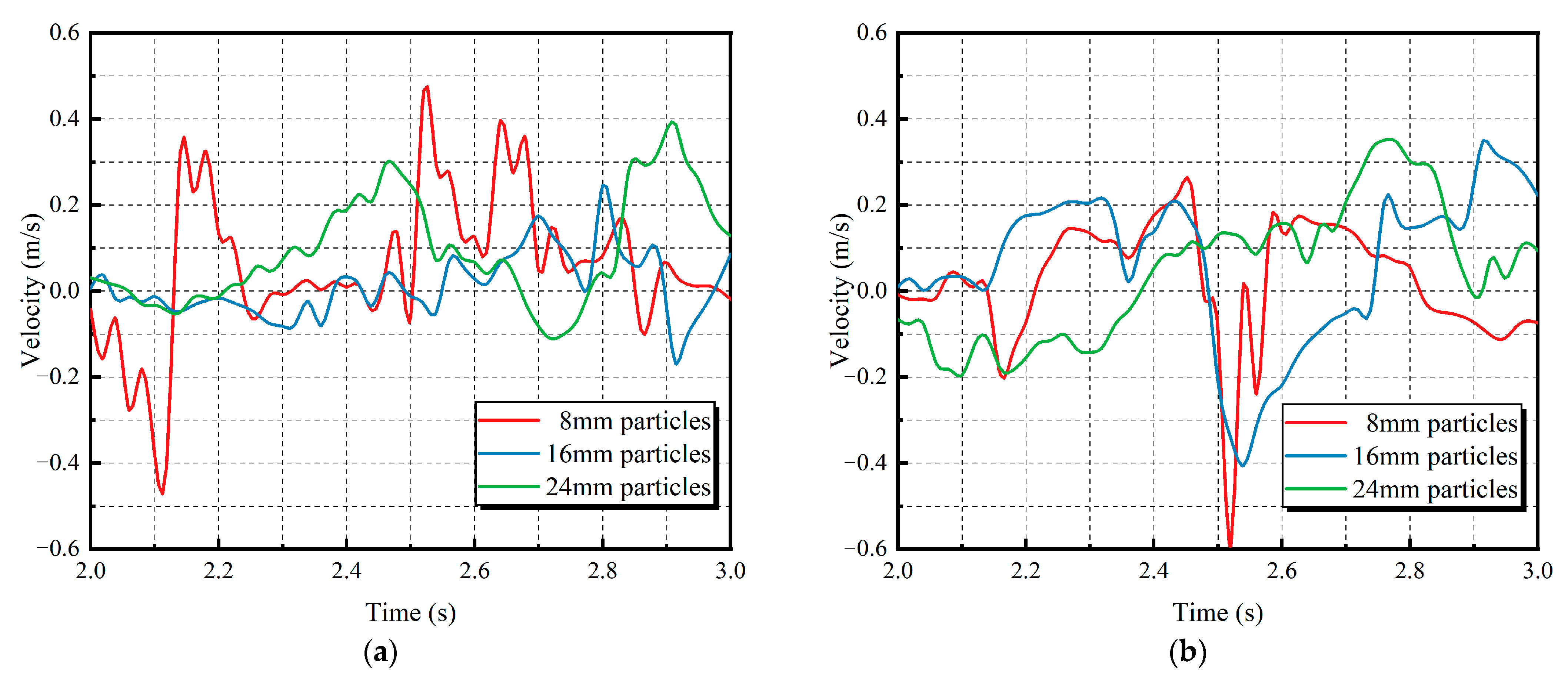
Figure 12 shows the trajectory and speed of partial particles and individual particles of different sizes when the initial flow velocity is 2 m/s, and the particle volume concentration is 6%. Figure 12a is a trajectory image of a part of the particles in the pipeline. Figure 12b–d are trajectory images of a single particle with diameters of 8 mm, 16 mm, and 24 mm, respectively. The lifting process of the particles in the pipe is not a linear movement, there is apparent lateral movement, and the particles may collide with the pipe wall. During the lifting process, the flow in the pipe is turbulent, and the particles are subjected to irregular fluid forces. At the same time, they are subjected to the contact force between the particles, resulting in an irregular motion. The movement speed of the particles also changes with the conveying process. Overall, the velocity of the particles tends to decrease along the axial direction. This is because the particles’ density is greater than that of seawater, and collisions between particles and particles cause a loss of kinetic energy. It can be seen from the image of a single particle that the speed of the particle decreases when it moves to the vicinity of the tube wall. The flow rate is reduced near the wall, and there is greater fluid resistance to the particles. Particles contacting the tube wall are affected by the contact force of the tube wall, which has a more significant impact on the velocity. When the particle size is small, the influence of multiple factors on its movement is more obvious.

After the particle flow in the pipeline is in a stable state, three adjacent particles of different sizes are selected near the entrance of the pipeline, and their respective lateral movement speeds are obtained. Figure 13 shows the change curve of the lateral velocity of each particle size particle with time when the initial flow velocity is 2 m/s and the particle concentration is 6%. Figure 13a shows the velocity in the x-axis direction, and Figure 13b shows the velocity in the y-axis direction. The figure shows that the lateral velocity of particles with a smaller particle size changes faster, and there is a sudden change in velocity. The lateral velocity changes of large particles are relatively stable. This corresponds to the particle velocity shown in Figure 12b–d. From the perspective of the entire lifting process, the lateral movement speed of small particles is greater than that of large particles, which conforms to the particle movement trajectory shown in Figure 12b–d. Particles with small particle sizes have less weight and are more likely to be affected and move laterally.

Figure 14 shows the trajectories and speeds of partial particles and individual particles of different sizes when the initial flow rate is 4 m/s, and the particle volume concentration is 6%.

Figure 14a is a trajectory image of a part of the particles in the pipeline. Figure 14b–d are trajectory images of a single particle with diameters of 8 mm, 16 mm, and 24 mm, respectively. With the increase of the flow rate, the amplitude of the lateral movement of the particles is obviously reduced, and the change of the movement speed is relatively small. When the flow rate is faster, the momentum exchange and energy exchange between the turbulence and the particles in the pipeline are more frequent, making the speed of the particles closer to the rate of the fluid, that is, reducing the sliding speed of the particles relative to the fluid. Simultaneously, the local concentration of particles is lower, and there are fewer collisions between particles and between particles and the pipe wall. The movement of particles at high flow rates is more stable than that at low flow rates. Figure 15 shows the change curve of the lateral velocity of each particle size particle with time when the initial flow velocity is 4 m/s and the particle concentration is 6%. Figure 15a shows the velocity in the x-axis direction, and Figure 15b shows the velocity in the y-axis direction. Compared with the case where the initial flow velocity is 2 m/s, the lateral velocity of particles of all diameters under this working condition has been significantly reduced, which corresponds to the reduced lateral displacement in Figure 14. Smaller particles also have a sudden change in speed at high flow rates, but the fluctuation range and change speed are relatively flat.

Figure 16 shows the trajectories and speeds of partial particles and individual particles of different sizes when the initial flow rate is 2 m/s, and the particle volume concentration is 12%. In the case of a large particle volume concentration, the particle’s motion trajectory has apparent rapid lateral displacement due to collision, and the movement speed also has sudden changes and repeated changes. When there are more particles, the contact force between the particles occurs more frequently. Particles are affected by complex forces in multiple directions, and the movement of the particles is more irregular. It can be seen from the single-particle images of various working conditions that the smaller the particle size, the more obvious the impact on the motion state after the contact force. Figure 17 shows the change curve of the lateral velocity of each particle size particle with time when the initial flow velocity is 2 m/s and the particle concentration is 12%. Due to more frequent collisions between particles, the lateral velocity changes of the particles become significantly more intense. The transverse velocity of the 8 mm particle has an obvious large fluctuation. Even the 24 mm diameter particle has larger lateral velocity values that did not appear in the previous two working conditions.

5.2. Slip Velocity

The difference between the particles moving rate in the axial direction and the conveying water flow rate is called the slip velocity, which is an important indicator of the stagnation effect in the hydraulic conveying process. The aggregation phenomenon caused by the hysteresis effect increases the local concentration. Therefore, the area where the particle velocity decreases is usually accompanied by particle aggregation, which is unfavorable for safe conveying.

Figure 18 shows the average slip velocity of particles in the pipeline under different working conditions. There is a slight overall increase in the slip velocity as the feed concentration increases. The effect of flow velocity on slip velocity is more significant. When V₀ ≤ 3 m/s, the slip velocity is not affected much by the increase of the inlet flow rate. And V₀ ≥ 3 m/s, the slip velocity decreases rapidly with the increase of inlet flow velocity. At V₀ = 5 m/s, the slip velocity is less than 0. All the above phenomena are consistent with the overall particle concentration distribution characteristics in Figure 6. At high flow velocity, the momentum exchange as well as energy exchange between turbulent flow and particles in the pipe is more frequent, and the average velocity difference between particles and fluid decreases. At the same time, the local concentration of particles is lower, so the collision between particles is reduced, and the kinetic energy loss of particles is reduced, so the slip velocity is reduced.

Since the high inlet flow rate inevitably increases the power demand on the pump, it is only necessary to control the slip velocity within a reasonable range. Therefore, about 4 m/s is the suitable inlet flow rate selection range.

6. Conclusions

In this paper, the effect of different operating parameters on the polymetallic nodule transport process is studied based on the CFD–DEM numerical simulation method. As a result of the study;

(1) Force analysis of solid–liquid two-phase flow based on the principle of fluid mechanics was conducted. A coupled CFD–DEM method based on Fluent and EDEM was established. A simulation model was established based on the actual deep-sea mining system and the physical properties of polymetallic nodules. It was verified, using small laboratory tests, that the model can reasonably simulate the process of hydrodynamic lifting of particles in the pipe.

(2) It was found that the hysteresis of particles in the pipeline is more pronounced at small inlet flow rates, large feed concentrations and coarse particle fragmentation levels, which increases the risk of particle aggregation and pipeline blockage. It is specifically reflected in the simulation results as: large overall concentration, large fluctuation of local concentration and radial concentration, unstable particle motion trajectory, and large slip velocity.

(3) The operating parameters of commercial deep-sea mining are set to meet the premise of safe and stable operation of the system to maximize the collection efficiency. Based on the simulation results, it is recommended that the inlet flow velocity of the transport pipeline be set at about 4 m/s, the initial concentration of particles be controlled at about 9%, and the particle size of the crushed polymetallic nodules be ensured to be within 16 mm. However, there are certain limitations in this study. The effect of particle degradation has not been fully considered. The particles will not be regularly spherical after the crushing process. There is a gap between the particle model in the simulation and the actual situation, which leads to insufficient accuracy in the analysis of particle contact effects. In future research, these aspects will be supplemented and expanded.

References

1. Valsangkar, A.B. Deep-sea polymetallic nodule mining: Challenges ahead for technologists and environmentalists. Mar. Georesour. Geotechnol. 2003, 21, 81–91. [Google Scholar] [CrossRef]
2. Cho, S.-G.; Park, S.; Oh, J.; Min, C.; Kim, H.; Hong, S.; Jang, J.; Lee, T.H. Design optimization of deep-seabed pilot miner system with coupled relations between constraints. J. Terramech. 2019, 83, 25–34. [Google Scholar] [CrossRef]
3. Yang, H.; Liu, S. Measuring Method of Solid-Liquid Two-Phase Flow in Slurry Pipeline for Deep-Sea Mining. Thalassas 2018, 34, 459–469. [Google Scholar] [CrossRef]
4. Dai, Y.; Li, X.; Yin, W.; Huang, Z.; Xie, Y. Dynamics analysis of deep-sea mining pipeline system considering both internal and external flow. Mar. Georesour. Geotechnol. 2021, 39, 408–418. [Google Scholar] [CrossRef]
5. Durand, R. Basic relationships of the transportation of solids in pipes-experimental research. Proc. Int. Assoc. Hydraul. Res. 1953, 83–103. [Google Scholar]
6. Wasp, E.J.; Kenny, J.P.; Gandhi, R.L. Solid-liquid flow: Slurry pipeline transportation. Ser. Bulk Mater. Handl. 1977, 1, 56–58. [Google Scholar]
7. Chung, J.S.; Lee, K.; Tischler, A.; Int Soc, O.; Polar, E. Two-phase vertically upward transport of silica sands in dilute polymer solution: Drag reduction and effects of sand size and concentration. In Proceedings of the Seventh ISOPE Ocean Mining Symposium, Lisbon, Portugal, 1–6 July 2007; pp. 188–196. [Google Scholar]
8. Yoon, C.H.; Lee, D.K.; Kwon, K.S.; Kwon, S.K.; Kim, I.K.; Park, Y.C.; Kwon, O.K. Experimental and numerical analysis on the flow characteristics of solid-liquid two-phase mixtures in a curvature pipe. In Proceedings of the Twelfth International Offshore and and Polar Engineering, Kitakyushu, Japan, 26–31 May 2002; pp. 475–479. [Google Scholar]
9. Yoon, C.-H.; Park, Y.-C.; Park, J.; Kim, Y.-J.; Kang, J.-S.; Kwon, S.-K. Solid-Liquid Flow Experiment with Real and Artificial Manganese Nodules in Flexible Hoses. Int. J. Offshore Polar Eng. 2009, 19, 77–79. [Google Scholar]
10. Vlasak, P.; Chara, Z.; Konfrst, J.; Krupicka, J. Concentration Distribution of Coarse-Grained Particle-Water Mixture in Horizontal Pipe. In Proceedings of the Engineering Mechanics 2014, Svratka, Czech Republic, 12–15 May 2014; pp. 684–687. [Google Scholar]
11. Kongar-Syuryun, C.B.; Faradzhov, V.; Tyulyaeva, Y.S.; Khayrutdinov, A. Effect of activating treatment of halite flotation waste in backfill mixture preparation. Min. Inf. Anal. Bull. 2021, 1, 43–57. [Google Scholar] [CrossRef]
12. Sobota, J.; Vlasak, P.; Petryka, L.; Zych, M. Slip velocities in mixture vertical pipe flow. In Proceedings of the Tenth ISOPE Ocean Mining and Gas Hydrates Symposium, Szczecin, Poland, 22–26 September 2013; pp. 221–224. [Google Scholar]
13. Boetius, A.; Haeckel, M. Mind the seafloor. Science 2018, 359, 34–36. [Google Scholar] [CrossRef] [PubMed]
14. Sobota, J.; Palarski, J.D.; Plewa, F.; Strozik, G. Analysis of Two-phase Mixture Flow In Vertical Pipeline. In Proceedings of the Seventh ISOPE Ocean Mining Symposium, Lisbon, Portugal, 1–6 July 2007. [Google Scholar]
15. Adigamov, A.; Zotov, V.; Kovalev, R.; Kopylov, A. Calculation of transportation of the stowing composite based on the waste of water-soluble ores. Transp. Res. Procedia 2021, 57, 17–23. [Google Scholar] [CrossRef]
16. Kongar-Syuryun, C.; Aleksakhin, A.; Khayrutdinov, A.; Tyulyaeva, Y. Research of rheological characteristics of the mixture as a way to create a new backfill material with specified characteristics. Mater. Today Proc. 2021, 38, 2052–2054. [Google Scholar] [CrossRef]
17. Masanobu, S.; Takano, S.; Fujiwara, T.; Kanada, S.; Ono, M.; Sasagawa, H. Study on Hydraulic Transport of Large Solid Particles in Inclined Pipes for Subsea Mining. J. Offshore Mech. Arct. Eng.-Trans. ASME 2017, 139. [Google Scholar] [CrossRef] [Green Version]
18. Van Wijk, J.M.; van Rhee, C.; Talmon, A.M. Wall friction of coarse grained sediment plugs transported in a water flow through a vertical pipe. Ocean Eng. 2014, 79, 50–57. [Google Scholar] [CrossRef]
19. Van Wijk, J.M.; van Grunsven, F.; Talmon, A.M.; van Rhee, C. Simulation and experimental proof of plug formation and riser blockage during vertical hydraulic transport. Ocean Eng. 2015, 101, 58–66. [Google Scholar] [CrossRef]
20. Van Wijk, J.M.; Talmon, A.M.; van Rhee, C. Stability of vertical hydraulic transport processes for deep ocean mining: An experimental study. Ocean Eng. 2016, 125, 203–213. [Google Scholar] [CrossRef]
21. Beauchesne, C.; Parenteau, T.; Septseault, C.; Béal, P.-A. Development & Large scale validation of a transient flow assurance model for the design & Monitoring of large particles transportation in two phase (Liquid-Solid) riser systems. Flow Assurance 2015, 4, 2790–2810. [Google Scholar]
22. Wang, L.; Liu, Z.Y.; Abdelkefi, A.; Wang, Y.K.; Dai, H.L. Nonlinear dynamics of cantilevered pipes conveying fluid: Towards a further understanding of the effect of loose constraints. Int. J. Non-Linear Mech. 2017, 95, 19–29. [Google Scholar] [CrossRef]
23. Yoon, C.-H.; Kang, J.-S.; Park, J.-M.; Park, Y.-C.; Kim, Y.-J.; Kwon, S.-K. Flow analysis by CFD model of lifting system for shallow sea test. In Proceedings of the Eighth ISOPE Ocean Mining Symposium, Chennai, India, 20–24 September 2009. [Google Scholar]
24. Xu, H.; Chen, W.; Hu, W. Hydraulic transport flow law of natural gas hydrate pipeline under marine dynamic environment. Eng. Appl. Comput. Fluid Mech. 2020, 14, 507–521. [Google Scholar] [CrossRef]
25. Liu, L.; Yang, J.; Lu, H.; Tian, X.; Lu, W. Numerical simulations on the motion of a heavy sphere in upward Poiseuille flow. Ocean Eng. 2019, 172, 245–256. [Google Scholar] [CrossRef]
26. Cundall, P.A.; Strack, O. A Discrete Numerical Model For Granular Assemblies. Geotechnique 1979, 29, 47–65. [Google Scholar] [CrossRef]
27. Akhshik, S.; Behzad, M.; Rajabi, M. CFD-DEM simulation of the hole cleaning process in a deviated well drilling: The effects of particle shape. Particuology 2016, 25, 72–82. [Google Scholar] [CrossRef]
28. Yuan, J.; Li, H.; Qi, X.; Hu, T.; Bai, M.; Wang, Y. Optimization of airflow cylinder sieve for threshed rice separation using CFD-DEM. Eng. Appl. Comput. Fluid Mech. 2020, 14, 871–881. [Google Scholar] [CrossRef]
29. Huang, S.; Su, X.; Qiu, G. Transient numerical simulation for solid-liquid flow in a centrifugal pump by DEM-CFD coupling. Eng. Appl. Comput. Fluid Mech. 2015, 9, 411–418. [Google Scholar] [CrossRef] [Green Version]
30. Chen, Q.; Xiong, T.; Zhang, X.; Jiang, P. Study of the hydraulic transport of non-spherical particles in a pipeline based on the CFD-DEM. Eng. Appl. Comput. Fluid Mech. 2020, 14, 53–69. [Google Scholar] [CrossRef]
31. Uzi, A.; Levy, A. Flow characteristics of coarse particles in horizontal hydraulic conveying. Powder Technol. 2018, 326, 302–321. [Google Scholar] [CrossRef]
32. Kloss, C.; Goniva, C.; Hager, A.; Amberger, S.; Pirker, S. Models, algorithms and validation for opensource DEM and CFD-DEM. Prog. Comput. Fluid Dyn. 2012, 12, 140–152. [Google Scholar] [CrossRef]
33. Hussainov, M.; Kartushinsky, A.; Mulgi, A.; Rudi, Ü. Gas-solid flow with the slip velocity of particles in a horizontal channel. J. Aerosol Sci. 1996, 27, 41–59. [Google Scholar] [CrossRef]
34. Karimi, H.; Dehkordi, A.M. Prediction of equilibrium mixing state in binary particle spouted beds: Effects of solids density and diameter differences, gas velocity, and bed aspect ratio. Adv. Powder Technol. 2015, 26, 1371–1382. [Google Scholar] [CrossRef]
35. Sakaguchi, H.; Ozaki, E.; Igarashi, T. Plugging of the Flow of Granular Materials during the Discharge from a Silo. Int. J. Mod. Phys. B 1993, 7, 1949–1963. [Google Scholar] [CrossRef]
36. Emeriault, F.; Cambou, B. Micromechanical modelling of anisotropic non-linear elasticity of granular media. Int. J. Solids Struct. 1996, 33, 2591–2607. [Google Scholar] [CrossRef]
37. Dai, Y.; Zhang, Y.; Li, X. Numerical and experimental investigations on pipeline internal solid-liquid mixed fluid for deep ocean mining. Ocean Eng. 2021, 220, 108411. [Google Scholar] [CrossRef]
38. Norouzi, H.R.; Zarghami, R.; Sotudeh-Gharebagh, R.; Mostoufi, N. Coupled CFD-DEM Modeling: Formulation, Implementation and Application to Multiphase Flows; John Wiley & Sons, Ltd.: Tehran, Iran, 2016. [Google Scholar]
39. Akbarian, E.; Najafi, B.; Jafari, M.; Ardabili, S.F.; Shamshirband, S.; Chau, K.-W. Experimental and computational fluid dynamics-based numerical simulation of using natural gas in a dual-fueled diesel engine. Eng. Appl. Comput. Fluid Mech. 2018, 12, 517–534. [Google Scholar] [CrossRef] [Green Version]
Figure 1. Contact force model between particles [37].
Sustainability 15 04248 g001
Figure 2. CFD–DEM coupling principle.
Sustainability 15 04248 g002
Figure 3. Layout of the experimental system [37].
Sustainability 15 04248 g003
Figure 4. Schematic diagram of particle trajectory tracking.
Sustainability 15 04248 g004
Figure 5. Comparison of particle trajectories under different initial flow rates: (a) V0 = 1.14 m/s; (b) V0 = 1.25 m/s.
Sustainability 15 04248 g005
Figure 6. Instantaneous overall particle concentration in the pipeline.
Sustainability 15 04248 g006
Figure 7. Particle distribution under V0 = 3 m/s and Cv = 9%: (a) even distribution; (b) small distribution; (c) medium distribution; (d) large distribution.
Sustainability 15 04248 g007
Figure 8. Local volume concentration over time: (a) V0 = 2 m/s; (b) V0 = 4 m/s.
Sustainability 15 04248 g008
Figure 9. Local volume concentration over time under V0 = 3 m/s and Cv = 9%: (a) even distribution; (b) small distribution; (c) medium distribution; (d) large distribution.
Sustainability 15 04248 g009aSustainability 15 04248 g009b
Figure 10. Radial distribution of particle volume concentration.
Sustainability 15 04248 g010
Figure 11. Radial concentration distribution of different particle sizes.
Sustainability 15 04248 g011
Figure 12. Particle trajectory and velocity under V0 = 2 m/s and Cv = 6%: (a) partial particles; (b) 8 mm particle; (c) 16 mm particle; (d) 24 mm particle.
Sustainability 15 04248 g012
Figure 13. Time-varying curve of particle lateral velocity under V0 = 2 m/s and Cv = 6%: (a) x-axis direction; (b) y-axis direction.
Sustainability 15 04248 g013
Figure 14. Particle trajectory and velocity under V0 = 4 m/s and Cv = 6%: (a) partial particles; (b) 8 mm particle; (c) 16 mm particle; (d) 24 mm particle.
Sustainability 15 04248 g014
Figure 15. Time-varying curve of particle lateral velocity under V0 = 4 m/s and Cv = 6%: (a) x-axis direction; (b) y-axis direction.
Sustainability 15 04248 g015
Figure 16. Particle trajectory and velocity under V0 = 2 m/s and Cv = 12%: (a) partial particles; (b) 8 mm particle; (c) 16 mm particle; (d) 24 mm particle.
Sustainability 15 04248 g016
Figure 17. Time-varying curve of particle lateral velocity under V0 = 2 m/s and Cv = 12%: (a) x-axis direction; (b) y-axis direction.
Sustainability 15 04248 g017
Figure 18. Average slip velocity of particles in the pipeline.
Sustainability 15 04248 g018