Application of Induced Polarization Method in Mineral Resource Exploration

Abstract

The search for hidden minerals with a large, buried depth depends on the guidance of geological and metallogenic theory, but it is difficult to master the geological characteristics of deep deposits. In this paper, taking a survey area as an example, the stimulated polarization geophysical method is used to obtain the information of deep minerals indirectly. Through the analysis and study of IP (induced polarization) anomaly and its characteristics in a tin polymetallic mining area, we delineate the IP anomaly distribution zone of metal ore, identify the distribution of polarized abnormal bodies by IP sounding, and determine the distribution of metallogenic fracture zones in the working area. Through the least square inversion of resistivity and polarizability, the spatial correspondence between the abnormal area of resistivity and polarizability and the location of ore bodies are obtained. The strategy of deep-mineral-induced polarization analysis adopted by us can provide a reliable geophysical basis for rapid deep geological prospecting.

1. Introduction

The time domain IP method is a geophysical method commonly used in geological exploration. The induced polarization method is a geophysical exploration method that uses the differences in conductivity and induced polarization characteristics of rock and ore to observe and study the change law of artificially formed induced polarization fields to carry out prospecting and solve other geological problems. The induced polarization method measures the secondary field, and the excitation power can be either DC power or AC power. For different target geological bodies, the physical property information reflected by IP parameters needs to be specifically analyzed. Due to the different electrode effects of different rocks and ores, the speed of secondary field attenuation is different. Therefore, the apparent polarizability, half decay time, and other parameters measured by charging and discharging effects can be combined with hydrogeological conditions and various other pieces of prior information for geological interpretation to detect the deep polymetallic mineralization of fluorite mineralization fault zones [1,2].

2. Geological Background

From 1977–1979, the Second Regional Survey Team of the Hebei Provincial Bureau of Geology carried out 1/200,000 regional geological survey works and made a detailed discussion on regional geology and minerals. In 1982, the 111 Geological Team of the Inner Mongolia Geological Bureau found that some altered rocks in this area have tin mineralization. From 1985–1986, the first geophysical and geochemical exploration team of the Inner Mongolia Geological Bureau carried out a comprehensive geophysical and geochemical survey in the region. At the beginning of 2009, the Inner Mongolia Geological Exploration Institute carried out systematic geological logging of surface engineering and inclined shafts in the mining area, and conducted deep control of tin mineralization bodies in the area. In the same year, Central South University carried out a systematic study on the metallogenic regularity of tin, copper, lead, zinc, and bismuth ore bodies in the mining area.

The above geological work has focused on the Qianjingou mining area from different angles, providing a basis for carrying out geological prospecting, mineral evaluation, and finding out the structural distribution characteristics in the mining area. According to the metallogenic geological characteristics and physical characteristics of the mineralized body, it is confirmed that the tungsten tin polymetallic ore body in this area is generally characterized by low resistance and high polarization.

2.1. Stratum

The stratum in the working area is exposed singly, mainly including the Mesozoic Upper Jurassic Zhangjiakou Formation (J₃z) and the Quaternary system (Q). The stratum of the Mesozoic Upper Jurassic Zhangjiakou Formation (J₃z) is widely exposed. The lithology is quartz trachyte and trachyte. The porphyritic structure with few and many spots is dominant, and the local structure is a non-porphyritic cryptocrystalline structure and massive structure. The Quaternary system is mainly distributed in the mountain depression and gully in the northwest of the work area and is accumulated by alluvial and slope sandy clay, fine sand, etc. The upper part is covered with aeolian sands, and the maximum thickness is approximately 10 m.

2.2. Magmatic Rock

Magmatic rock mainly includes granite porphyry (λ_π52⁽³⁾), which is a small branch of porphyritic granite. It is mainly exposed in the southeast region of the exploration area and the west of the exploration area and intrudes into the trachyte and quartz trachyte of the second member of Zhangjiakou Formation (J₃). Its overall shape is a long strip with a porphyritic texture. Its phenocryst content is generally 15–20%, mainly composed of quartz and feldspar.

2.3. Ore Type and Structural Characteristics

Tin ore is distributed in the dense jointed zone and fractured zone in the form of fine veins, net veins and, disseminated. The ore type is mainly cassiterite quartz vein type. The ore minerals are mainly cassiterite with a small amount of wolframite and bismuthinite. The gangue minerals are quartz, sericite, and a small amount of feldspar, fluorite, calcite, etc.

Tungsten ore is mainly fine vein, disseminated, and then massive, distributed in strongly altered rocks in internal and external contact zones, and the ore type is quartz wolframite. Bismuth ores are distributed in the fractures and fracture zones of the outer contact zone in the form of veinlet and disseminated. The ore type belongs to the quartz vein type. The ore minerals are mainly bismuthinite and wolframite. The gangue minerals are mainly quartz, fluorite, and calcite.

Brass ore is distributed in the carbonated fracture zone and the fracture zone of the internal and external contact zones in the form of a veinlet shape, vein, and disseminated. The ore type belongs to a vein copper deposit, which is distributed in strongly silicified and carbonated quartz trachyte in the outer contact zone. Lead zinc ores are in vein and veinlet shapes, mainly distributed in the outer contact zone, carbonated fracture zone, and fracture zone. The ore type is a vein lead–zinc ore and the ore minerals are mainly galena, sphalerite, and a small amount of chalcopyrite. Gangue minerals are mainly carbonate and quartz.

2.4. Wall Rock Alteration

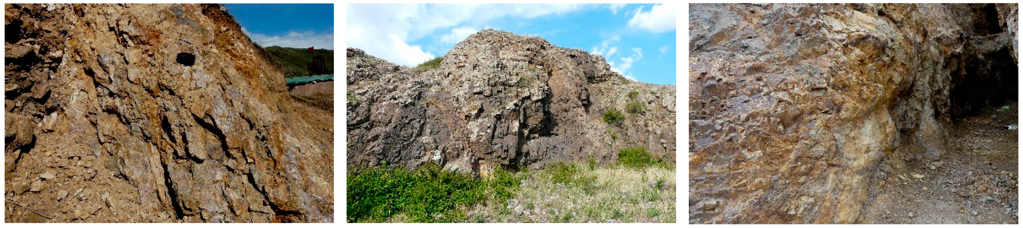
On the internal and external contact zone of porphyritic granite, rock alteration is widespread. The alteration types are mainly silicification and sericitization, followed by chloritization, carbonation, potassium, sodium, fluorization, and electrification. Potassium and sodium are mainly distributed in the inner contact zone. Silicification, sericitization, carbonation, and chloritization are mainly distributed in the outer contact zone. Tin ore bodies, tungsten ore bodies, and bismuth pyroxene ore bodies are mainly distributed in the strongly silicified alteration zone. Chalcopyrite, galena, and zinc-blended ore bodies are mainly distributed in moderately silicified, carbonated, and fluoritized alteration zones.

Intensive silication, sericitization, and pyritization are important indicators for prospecting in this area. Figure 1 shows some petrographical pictures.

3. Electrical Characteristics of Rock and Ore

The physical property of rocks is an important basis for anomaly interpretation, and the collection of physical property samples is an important link in geophysical exploration. In order to understand the polarization characteristics of various rocks in the work area, exposed rock samples were collected in the work area for physical property measurement. A total of 57 physical samples were collected, including 19 fluorite ores, 14 trachyte mines, 15 silicified altered trachyte mines, 6 polymetallic ores, and 3 tungsten mineralized quartzite mines. The polarizability of these samples was measured.

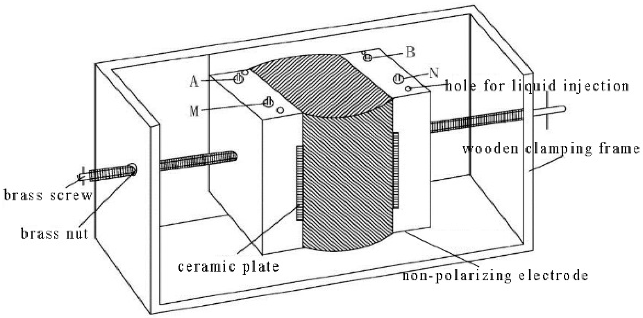
Before the determination, the above physical property samples were soaked in water for 24 h and the determination was completed within 6 h after the samples were taken out and dried. The polarizability of physical samples is measured by the specimen rack method, and the measured parameters are similar to those of field measurements. The specimen rack is composed of two parts. One is the clamping frame, which is used to hold and clamp the specimen to be tested, the other contains two non-polarizing electrodes, each with power supply and measuring electrodes. See Figure 2 for specimen rack. See

Table 1. Physical properties of rock and ore.

Name of Rock and Ore	Block Number	Polarity (%)
		Mean	Min	Max
Fluorite ores	19	2	0.9	3.3
Trachyte mines	14	2.1	1.3	3
Silicified altered trachyte mines	15	2.7	1.9	3.8
Polymetallic ores	6	4.9	4.5	5.4
Tungsten mineralized quartzite mines	3	3.1	2.7	3.3

Note: The IP simulator was used as a small power transmitter to coordinate with the receiver for measurement. The polarizability of rock samples was measured using the working parameters consistent with those in the field.

for the measurement results.

Polymetallic ores had the highest polarizability with an average of 4.9%. Tungsten mineralized quartzite mines took the second place with an average of 3.1%. Furthermore, the polarizability of trachyte mines, which was the main part of bedrock in the area, was only 2.1%. However, when it underwent silicified alteration due to the ore-forming geological process, its polarizability increased, with an average of 2.7%. The fluorite ores in the area had the lowest polarizability among all kinds of rocks and ores but had a large range of variation, with polarizability values ranging from 0.9% to 3.3%. Theoretically, the induced polarization effect of fluorite should be very weak, so its polarizability should be low. The high polarizability of fluorite ore in this area might be due to the fluorite associated with other metal sulfides in local sections. Although the polarizability of the Quaternary sandy soil layer widely distributed in the area had not been measured, both theory and practice show that the polarizability of the sandy soil layer is low.

To sum up, the metal ores in the area had high polarizability. When they have a certain scale, they will cause a high-intensity apparent polarizability anomaly. The polarizability value of fluorite ore varies widely. In the fluorite mineralized area, either high value anomaly or low value anomaly might occur. Trachyte mines had low polarizability, which will show as the background field of apparent polarizability. However, the value of apparent polarizability will increase after its alteration and the apparent polarizability anomaly with weak strength may appear. Therefore, it was feasible to use the induced polarization method to search for deep polymetallic mineralization in this work area.

In addition, although the resistivity of rock ore was related to its material composition and structure, it was also closely related to its water content. Generally, the fracture structure will present a relatively low value of apparent resistivity. According to the aforementioned geological and mineral characteristics, the tin polymetallic mineralized bodies in this area showed moderate resistivity characteristics. On the one hand, they are controlled by the fault structure and filled in the fault fracture zone and the metal minerals as electronic conductors will enhance their conductivity. On the other hand, it was strongly silicified which increased its resistivity [3].

4. Line Layout

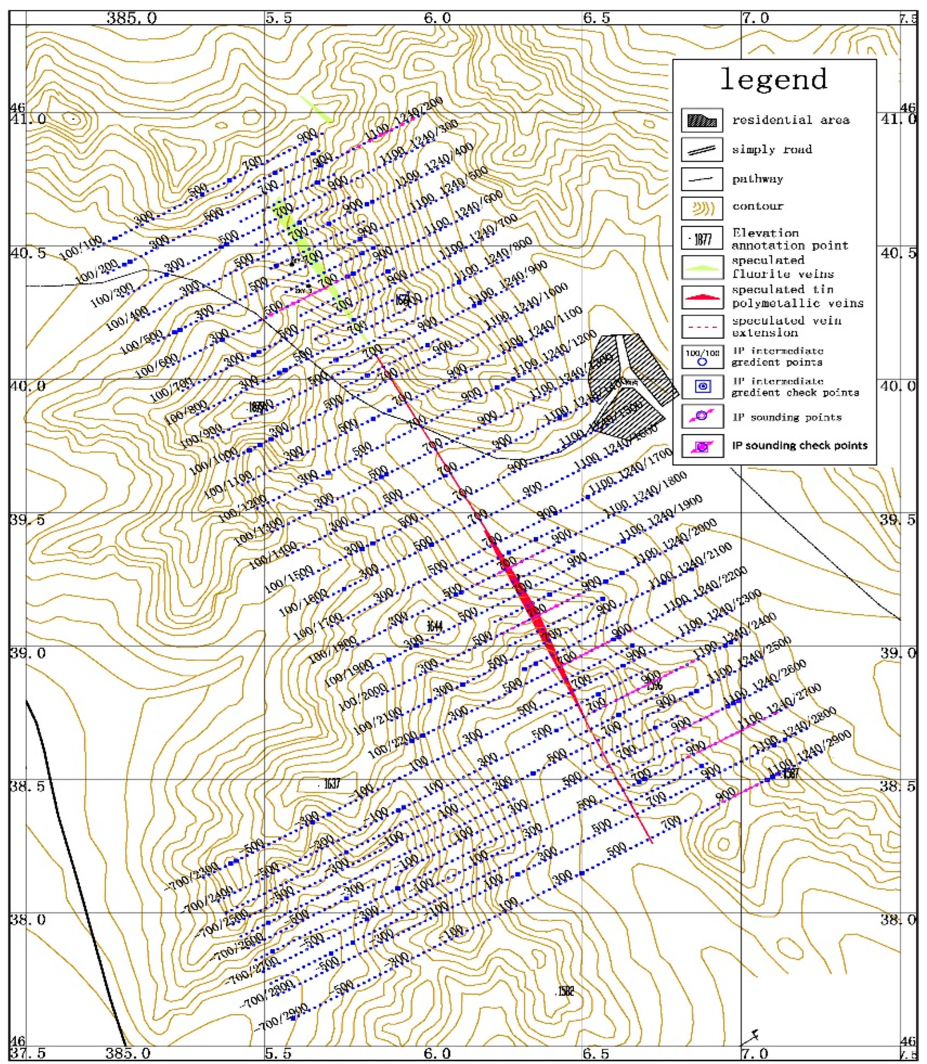
According to the geological condition of this area and the requirements of geological tasks, the IP intermediate gradient survey line in the NNE orientation was arranged vertically to the ore vein. The survey lines were distributed in parallel with a line distance of 100 m and a point distance of 20 m. The distance between lines and points in the survey area was 50 m and 20 m, respectively. The design section of IP intermediate gradient was 39.56 km long, with 1638 measuring points. See Figure 3 for details.

In order to correctly delineate the anomalies in the design work area, the survey area was expanded to a certain extent on the basis of the original design scope in the actual exploration work, and a total of 49.16 km IP intermediate gradient profiles, 2122 survey points, and 120 inspection points were completed. In this work, the IP sounding method was selected as an auxiliary method to check the anomalies of aerial work in the survey area. A total of 103 IP sounding survey points and six inspection points were completed. In addition, 57 physical samples of rocks exposed in the work area were collected and their polarizability was measured to understand the polarizability characteristics of various rocks in the work area [4].

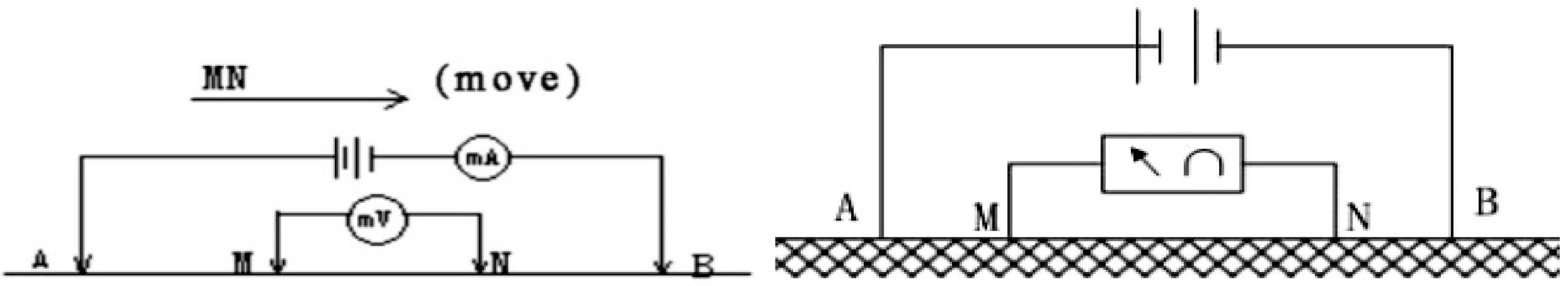
The power supply pole distance of the IP intermediate gradient was 1800 m and the power supply current was not less than 3A. The A and B pole power supply electrodes were arranged in a circular manner, with a total number of 50–60 electrodes. The adjacent power supply pole distance was equivalent to the buried depth of the electrodes. The measuring electrode distance was 40 m and the receiving electrode adopted solid non-polarizing electrodes. A two-way short pulse system supplied power with a duty cycle of 1:1. The power supply pulse width was ±4 s. The period was 16 s, the acquisition delay was 100 ms, the integration area was 50 ms, and the synchronization mode was self-synchronization [5]. See Figure 4 for the deployment diagram of IP intermediate gradient and IP sounding.

AB distance and MN distance shall be based on the principle of obtaining a complete electrical sounding curve and meeting the needs of interpretation. The standard of AB distance is based on the principle of making asymptotes appear at both ends of the electric sounding curve. The ratio of MN distance and AB distance is between 3/1 and 1/10. On the premise of meeting the point power supply, the power supply current shall be increased to ensure the acquisition of observation signals with a high signal-to-noise ratio.

IP sounding used a symmetrical quadrupole device. The setting of power supply and receiving parameters was the same as that of the IP intermediate gradient. However, the power supply current was adjusted with the power supply pole distance and the measurement pole distance. The pole distance variation of power supply polar distance is AB/2 and the receiving pole distance is MN/2. See

Table 2. Pole distance of IP sounding (unit: m).

AB/2	3	6	9	15	22	32	45	60	85	120	180	250	350	500	750
MN/2	1	1	1	1	1
				5	5	5	5	5	5
								20	20	20	20	20
											50	50	50	50	50

for pole distance of IP sounding.

Based on the analysis of the gradient surface results of IP, the IP anomaly areas with metallogenic significance were selected [6]. As an auxiliary method, IP sounding was mainly arranged in the above IP anomaly area to understand the buried depth, shape, and occurrence state of hidden anomaly bodies.

5. Data Processing

5.1. Measurement

According to the requirements of geophysical and geochemical engineering survey specifications, CASS, AutoCAD, and other software were used to organize and edit the survey data obtained and the actual material map of electrical prospecting was drawn, which included IP ladder points, IP sounding points, and check points. Refer to Figure 3 mentioned above.

5.2. IP Intermediate Gradient

We calculated the device coefficient K and apparent resistivity according to the AB distance, MN distance, and the distance between the side section and the main section and calculate the apparent resistivity of each measuring point. AM, BM, AN, and BN are the distances from the power supply points A and B to points M and N, respectively. The calculation formula of K on the main section is Formula (1) and the calculation formula of apparent resistivity is Formula (2) [7,8].

$$K=\frac{2\pi }{\frac{1}{AM}-\frac{1}{AN}-\frac{1}{BM}+\frac{1}{BN}}$$

(1)

$${\rho }_s=K\frac{\Delta U}{I}$$

(2)

In Formulas (1) and (2), K is the device coefficient; AM, BM, AN, and BN are the distances from the power supply points A and B to points M and N, respectively; ρ_s is apparent resistivity; and I is the current value emitted through the AB electrode.

We drew the profile plan of apparent resistivity and apparent polarizability. Without data processing, the profile plan can truly reflect the characteristics of the geoelectric field in the exploration area and can more clearly identify and analyze weak anomalies. The contour plan was one of the important maps in the interpretation of achievements. Through the contour map plane, we can clearly grasp the scope, amplitude, transformation gradient, and abnormal shape of each anomaly in the exploration area. When drawing an isoline plan or undertaking other post-processing, the data are required to be distributed on a regular grid. However, due to point location errors in the field measurement process, or because some points cannot be measured due to external reasons, the data obtained cannot be distributed on a regular grid. Therefore, the data shall be gridded before drawing, and the actual measured values on the irregular grid shall be converted to the values on the regular grid nodes. The Kriging grid method is used for this and the grid node spacing is 20 m.

5.3. IP Sounding

The symmetrical quadrupole sounding method was adopted for this IP sounding. With the increase in power supply electrode distance, it is necessary to increase the measuring electrode distance appropriately. However, when the measuring pole distance is changed, the apparent polarizability and apparent resistivity values observed at the same supply pole distance will be different. Therefore, when changing the measuring pole distance, it is necessary to observe the measured values before and after changing the measuring pole distance of at least two power supply poles, to ensure that the observation value changes with a certain rule before and after changing the measuring pole distance. During data processing, only one observation value is allowed for each power supply pole distance, and symmetric quadrupole sounding is based on the assumption that the measuring electrode distance is infinitesimal. Therefore, before processing the sounding data, all data must be converted into the observation value with the smallest measuring pole distance according to the change characteristics of the observation data at the junction point. There are many methods of joint point conversion [9].

In this case, it was assumed that the observation values of two power supply poles were remeasured before measuring the pole distance of MN for a certain change, which were a₁ and b₁, respectively. After transforming MN, the observation values of two power supply poles were a₂ and b₂. We used these four measured values to calculate a coefficient c, and then multiplied all the data after transforming MN by this coefficient to achieve the conversion purpose. The calculation method of c value is shown in Formula (3).

$$c=\frac{a_1+b_1}{a_2+b_2}$$

(3)

The deep geological body in this working area has a complex production and diverse structure. When studying the geoelectrical characteristics of the exploration line section, we should not only consider the longitudinal electrical change, but also the transverse electrical change. For this purpose, the inversion of the excited electrical data should be based on a two-dimensional basis.

5.3.1. Least Square Method for Two-Dimensional Resistivity Inversion

In the resistivity solution domain of the two-dimensional geoelectric section, each grid unit corresponded to a resistivity model parameter and the measured apparent resistivity pseudo section map corresponded to several sampling values of apparent resistivity. On this premise, the essence of two-dimensional resistivity inversion is to approach the measured pseudo section by constantly modifying the resistivity value in the grid unit of the geoelectric model under certain mathematical rules. In the process of approximation, the error between the theoretical value of apparent resistivity and the measured value was kept as small as possible by constantly modifying the model parameters, which was used as the standard to evaluate the degree of fitting.

The objective function solved is:

$$F={\displaystyle \sum }_{i=1}^N{\left[ln{\rho }_i^{measured}-ln{\rho }_i^{theoretical}\right]}^2=min$$

(4)

In the above formula, the apparent resistivity ${\rho }_i^{theoretical}$ is the result obtained through forward calculation of the initial value of the resistivity model, and it is a function related to the resistivity model parameters and the electrode distance of the device.

$${\rho }_i^{measured}={\rho }_i^{theoretical}\left(\rho ,d_i\right)$$

(5)

The problem of least squares in Formula (4) is nonlinear and it is difficult to obtain the model parameters directly by using the nonlinear function F. Therefore, it is necessary to linearize the nonlinear problem. The initial values are given according to the physical property data of the mining area and the program automatically calculates this. The initial value of model parameters given by the two-dimensional resistivity section is assumed to be ${\rho }^0=\left({\rho }_1^0,{\rho }_2^0,\cdots \cdots ,{\rho }_M^0\right)$. Expanding $ln{\rho }^{theoretical}\left(\rho ,d_i\right)$ in the form of Taylor series at ${\rho }^0$, and ignoring the partial derivative term greater than or equal to the second order:

$$ln{\rho }^{theoretical}\left(\rho ,d_i\right)\approx ln{\rho }^{theoretical}\left({\rho }^0,d_i\right)+{{\displaystyle \sum }}_{j=1}^M[\frac{\partial ln{\rho }^{theoretical}\left(\rho ,d_i\right)}{\partial {\rho }_j}{|}_{{\rho }^0}({\rho }_j-{\rho }_j^0)]$$

(6)

In Formulas (4) and (5), M and N are changed model parameters and d_i is electrode distance.

Make Formula (6) $\left\{\begin{array}{c}{a}_{ij}=\frac{\partial ln{\rho }^{theoretical}\left(\rho ,d_i\right)}{\partial {\rho }_j}\left|{ }_{{\rho }^0}\right. \left(i=1,2,\cdots \cdots N;j=1,2,\cdots \cdots ,M\right)\\ \Delta {\rho }_j={\rho }_j-{\rho }_j^0 \left(j=1,2,\cdots \cdots ,M\right) \end{array}\right.$.

Then, Formula (6) can be expressed as:

$$ln{\rho }^{theoretical}\left(\rho ,d_i\right)\approx ln{\rho }^{theoretical}\left({\rho }^0,d_i\right)+{\displaystyle \sum }_{j=1}^M{a}_{ij}\Delta {\rho }_j$$

(7)

Then, the linear approximate expression $F^{*}$ of the nonlinear objective function F can be obtained:

$$F^{*}={\displaystyle \sum }_{i=1}^N[ln{\rho }_i^{measured}-ln{\rho }_i^{theoretical}\left({\rho }^0,d_i\right)-{\displaystyle \sum }_{j=1}^M{a}_{ij}\Delta {\rho }_j{]}^2=min$$

(8)

The necessary condition for the existence of the minimum of $F^{*}$ is:

$$\frac{\partial F^{*}}{\partial \Delta {\rho }_k}=2{\displaystyle \sum }_{i=1}^N[ln{\rho }_i^{measured}-ln{\rho }_i^{theoretical}\left({\rho }^0,d_i\right)-{\displaystyle \sum }_{j=1}^M{a}_{ij}\Delta {\rho }_j]\left(-a_{ij}\right)=0 \left(k=1,2,\cdots \cdots ,M\right)$$

(9)

The above formula is expressed as:

$${\displaystyle \sum }_{i=1}^N{\displaystyle \sum }_{j=1}^M{a}_{ij}{a}_{ik}\Delta {\rho }_j={\displaystyle \sum }_{i=1}^N[ln{\rho }_i^{measured}-ln{\rho }_i^{theoretical}\left({\rho }^0,d_i\right)]a_{ik} \left(k=1,2,\cdots \cdots ,M\right)$$

(10)

The above formula can be changed into matrix form, namely:

$$A^{T}A\Delta \rho =A^{T}A\Delta G$$

(11)

In Formula (11), $\Delta G$ is the column vector with element $\Delta g_i=ln{\rho }_i^{measured}-ln{\rho }_i^{theoretical}\left({\rho }^0,d_i\right) \left(i=1,2,\cdots \cdots N\right)$. N×M-order coefficient matrix A is called the Jacobian matrix. The correction $\Delta \mathsf{\rho }$ of model parameters can be obtained by solving the normal equation.

To ensure the convergence of the inversion calculation process, the improved Fournier least square method (Marquette method) is used to enhance the numerical stability of Formula (11):

$$(A^{T}A+\lambda S)\Delta \rho =A^T\Delta G$$

(12)

In Formula (11), λ is the damping factor, which is used to constrain Formula (11) and enhance the numerical stability. S is the diagonal matrix:

$$S=\left[\begin{array}{ccc}\frac{1}{{\rho }_1^2}& & \begin{array}{cc} & \end{array}\\ \begin{array}{c} \\ \end{array}& \begin{array}{c}\frac{1}{{\rho }_2^2}\\ \end{array}& \begin{array}{c}\begin{array}{cc} & \end{array}\\ \begin{array}{cc}\cdots & \end{array}\end{array}\\ & & \begin{array}{cc} & \frac{1}{{\rho }_m^2}\end{array}\end{array}\right]$$

(13)

If $\Delta \mathsf{\rho }$ fails to reach the given accuracy, then demand ${\rho }^1={\rho }^0+\Delta \rho$, and repeat the above process with the new model ${\rho }^1$ instead of ${\rho }^0$, and iterative repeatedly until ${\rho }^k \left(k=1,2,\cdots \cdots ,M\right)$ meets the accuracy requirements [7].

5.3.2. Inversion of Polarizability

According to the theory proposed by Seigel in 1959, if the two-dimensional section is composed of N units, the apparent polarizability can be expressed as:

$${\eta }_{xi}={\displaystyle \sum }_{j=1}^M\left[\frac{\partial ln{\rho }_{xi}}{\partial {\rho }_j}\right] \left(x=1,2,\cdots ,N\right)$$

(14)

The matrix form is:

$${\eta }_x=A\eta$$

(15)

In Formula (15), ${\eta }_x$ is the vector of apparent polarizability, $\eta$ is the polarizability vector formed by each model unit, and A is the Jacobian matrix mentioned above.

It can be seen that the polarization inversion method of the two-dimensional section is the same as that of the resistivity inversion. The polarization distribution of the geoelectric section can be obtained by using the claw least square method through multiple iterations [10].

The geophysical model (the position and shape of the field source) is solved through the observation data (the distribution of the field), and under a certain mathematical premise, the observed values can be matched to the theoretical calculated values of the model to the maximum extent.

6. Abnormal Characteristics

In Section 5, we delineated and divided the anomalies of apparent metal factors and then explained the key anomalies in Section 6 to determine the anomaly areas with good geological prospecting prospects.

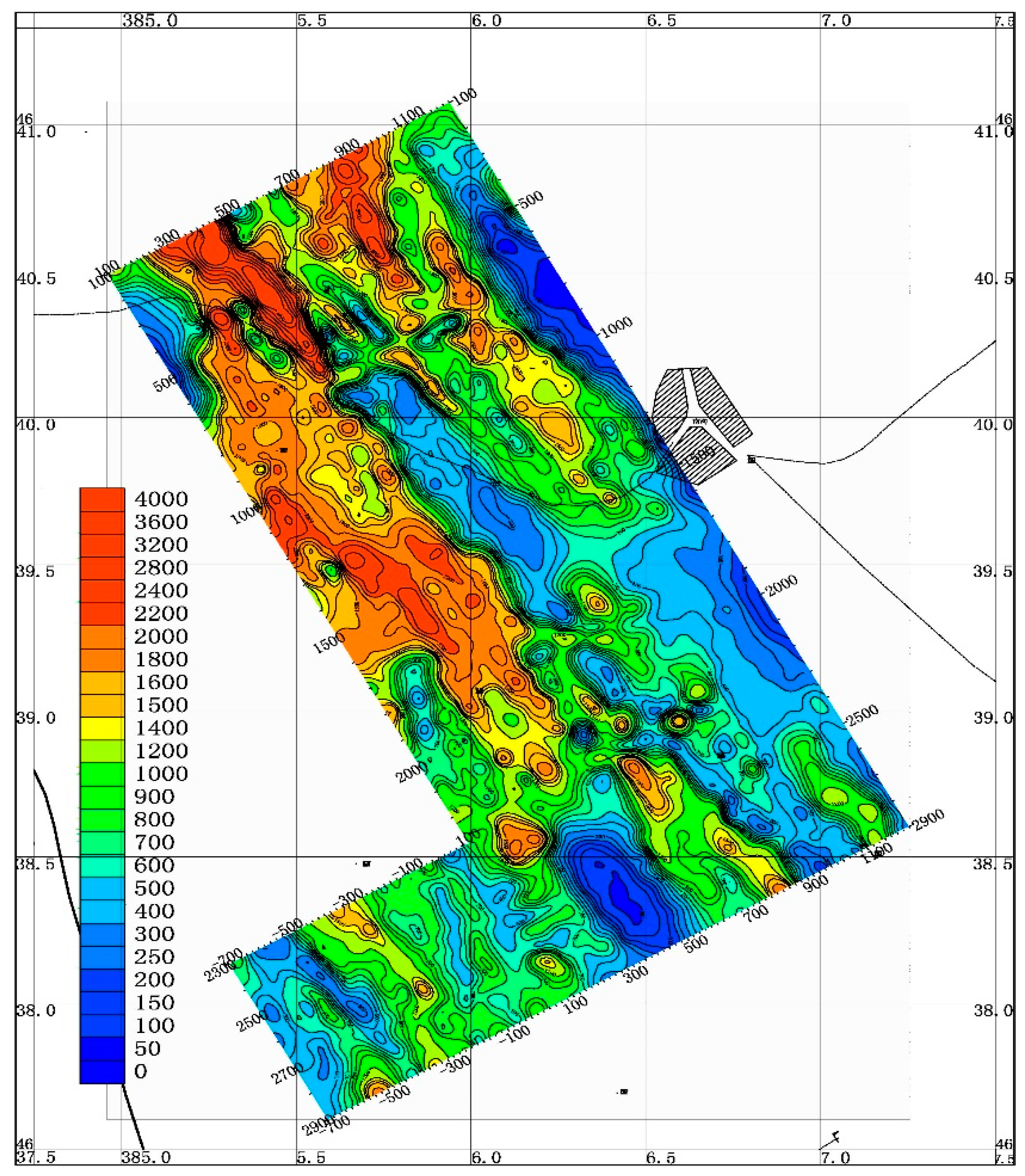
6.1. Plane Characteristics of Apparent Resistivity

We calculated the device coefficient K and apparent resistivity according to the AB distance, MN distance, and the distance between the side section and the main section and calculated the apparent resistivity of each measuring point. AutoCAD and Surfer were used to jointly prepare the contour plan, which mainly includes creating new graphic documents, gridding, generating contour maps, filling color codes, and modifying pictures.

It can be seen from the plane contour map of apparent resistivity (Figure 5) that the contour is distributed in the northwest direction, and the apparent resistivity in the whole area was distributed in high and low phases from southwest to northeast. According to the field survey, the high value areas with an apparent resistivity greater than 1400 Ω·m are all distributed in the exposed bedrock area or the section with thin Quaternary sediments, while the low value areas with apparent resistivity are distributed in the section with thick Quaternary sediments. Clearly, the change of apparent resistivity in this area has a close inverse correlation with the thickness of Quaternary sediments, that is, the greater the thickness of Quaternary sediments, the lower the apparent resistivity, and vice versa. However, in the extremely low value area of apparent resistivity, in addition to the influence of thicker Quaternary systems, the superposition effect caused by the fracture structure fracture zone was not excluded [11,12].

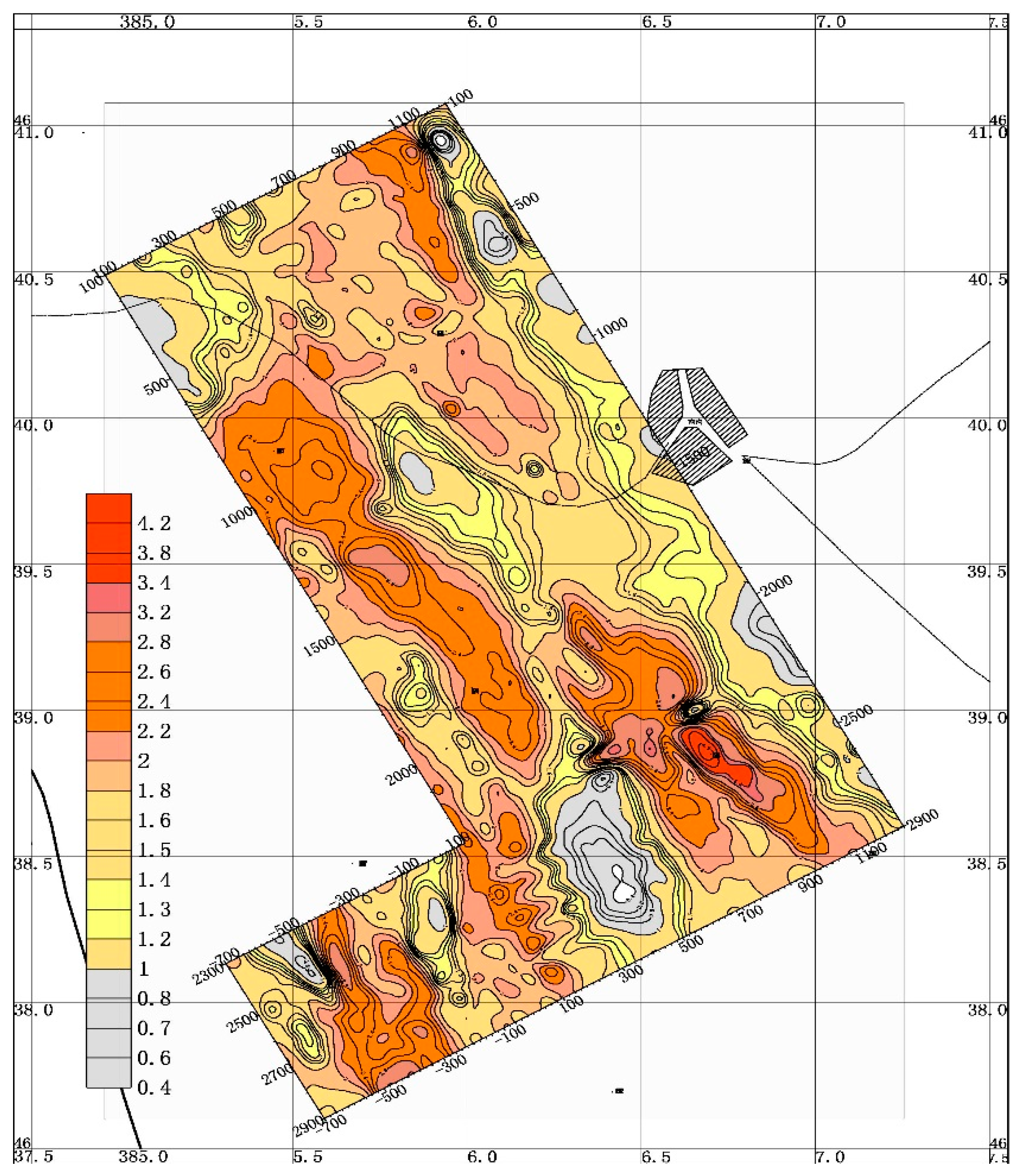
6.2. Distribution Characteristics of Apparent Polarizability

It can be seen from the plane contour map of apparent polarizability (Figure 6) that the area with apparent polarizability less than 2% constitutes the background field area of this area, and the apparent polarizability also shows that the main body of the contour was distributed in the northwest direction. The apparent polarizability of the whole area was characterized by alternating high and low distribution from southwest to northeast. High value areas with apparent polarizability greater than 2% are distributed in exposed bedrock areas or sections with thin Quaternary sediments, while low value areas with apparent polarizability are distributed in sections with thick Quaternary sediments. However, in the high value area of apparent polarizability and the local high value area in the low background field area, in addition to the influence of the small thickness of the Quaternary system, the superimposition of mineralization and alteration was not ruled out [13].

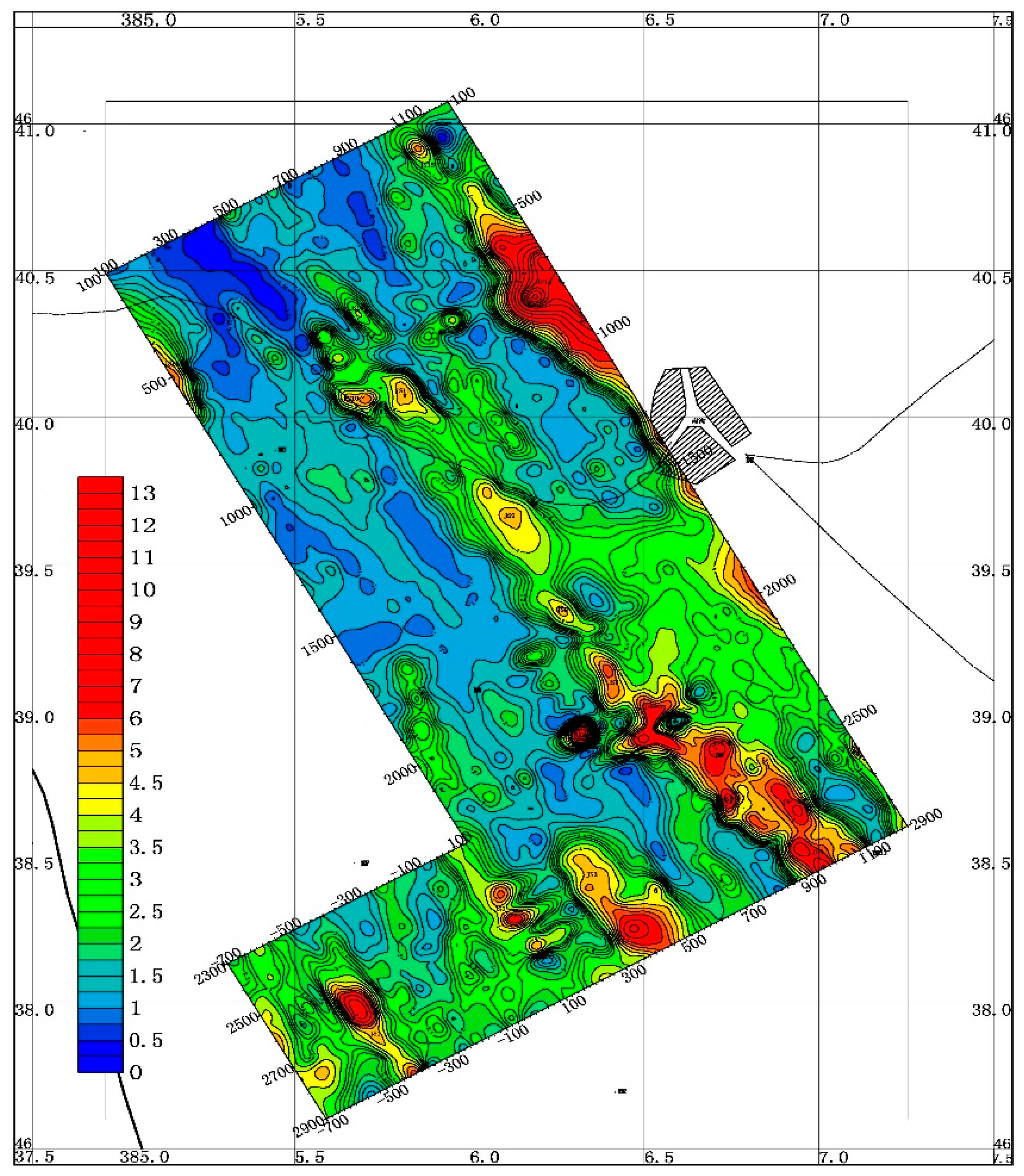
6.3. Relationship between Abnormal Area and Mineralization Alteration

Through comprehensive analysis of the results of apparent resistivity and apparent polarizability, both apparent resistivity and apparent polarizability anomalies reflect the known fluorite ore (mineralization) and tin polymetallic ore (mineralization). However, there are features of wide and wide range of anomalies, and the corresponding relationship between the anomalies of the two parameters and the known mineralization and alteration sections was not unique. Neither the apparent resistivity nor the apparent polarizability anomaly had accurately positioned the mineralized alteration section. From the electrical characteristics of rocks and ores in this area, it can be seen that tin polymetallic ore (mineralization) and fluorite ore (mineralization) in this area had high polarizability. Considering that the mineralization in this area was controlled by the fault structure, the apparent resistivity should be characterized by medium low resistance. That is to say, the mineralization alteration section in this area should have the characteristics of medium low resistance and high polarization. Based on this, the comprehensive parameter “apparent metal factor” (Figure 7) was obtained. This parameter was the ratio of apparent polarizability to apparent resistivity, which can better reflect the medium with low resistance and high polarization [14].

It can be seen from the figure that the apparent metal factor anomaly range of low resistance and high polarization delineated by 3 × 10⁻⁴ S/m as the minimum value was greatly reduced. The small-scale ore block near 800/2100~880/2600 points in the working area also confirmed that Figure 7 had a good correspondence.

We carefully analyzed the geological and metallogenic characteristics of this area, comprehensively compared and analyzed the delineated apparent metal factor anomaly with the apparent resistivity and apparent polarizability data and delineated the anomaly area with certain prospecting significance [15].

7. Inversion and Interpretation

The anomaly center was located near 800/2100 points to 880/2600 points in the work area (white solid coil in Figure 7). The abnormal shape delineated was irregular when the metal factor JS was 5 × 10⁻⁴ S/m. The delineated abnormal high values can be divided into three elliptical local anomalies in the north and south when the metal factor JS overtook 6 × 10⁻⁴ S/m. Among them, the long axis of abnormal JS5-3 in the north was approximately 200 m long, the short axis was approximately 70 m long, the long axis strikes near SN, and the highest value of apparent metal factor was greater than 7 × 10⁻⁴ S/m. The long axis of abnormal JS5-2 in the middle was approximately 150 m long, the short axis was approximately 100 m long, the long axis direction was northwest, and the highest value of apparent metal factor was also greater than 7 × 10⁻⁴ S/m. The area of abnormal JS5-1 in the south was small. It can be seen from Figure 5 and Figure 6 that the low value abnormal area of plane apparent resistivity (the minimum value of apparent resistivity was lower than 250 Ω·m) and the high value area of apparent polarizability (the maximum value of apparent polarizability was greater than 2.8%) corresponded to them [16].

The bedrock in the abnormal area was Zhangjiakou Formation quartz trachyte. Two IP sounding profiles were arranged on the 2200 and 2400 lines in the abnormal area in order to understand the deep mineralization.

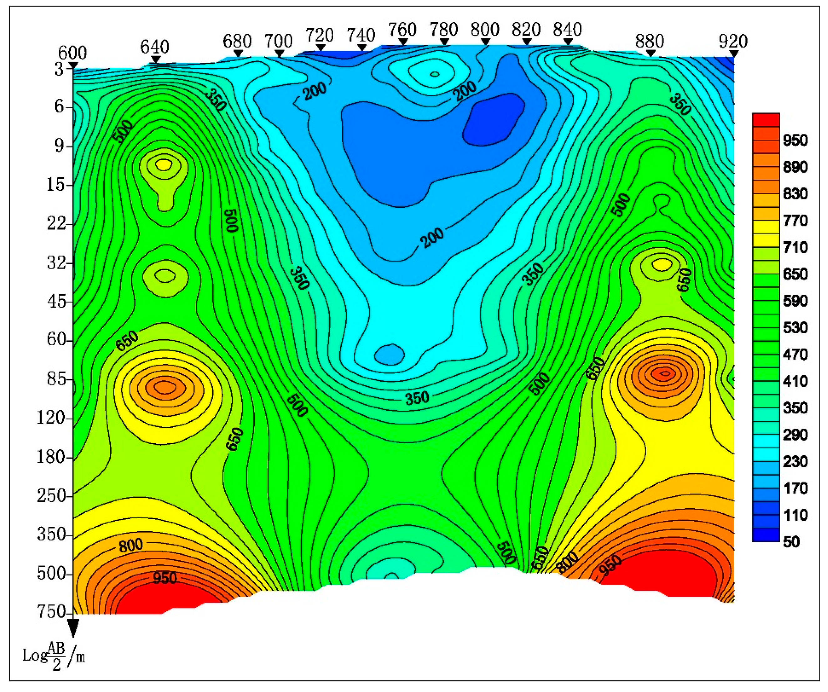
It can be seen from the apparent resistivity section of 2200 line IP sounding (Figure 8) that the apparent resistivity increased gradually as the power supply pole distance increased. When AB/2 < 85 m, the lateral change in apparent resistivity was large, indicating that the heterogeneity of shallow rock strata in this area was obvious, which was mainly caused by the thickness change in Quaternary sediments and the difference in bedrock weathering degree. When AB/2 > 85 m, the lateral change in apparent resistivity slowed down obviously, indicating that the homogeneity of deep rocks in this area was a good prospect [17,18].

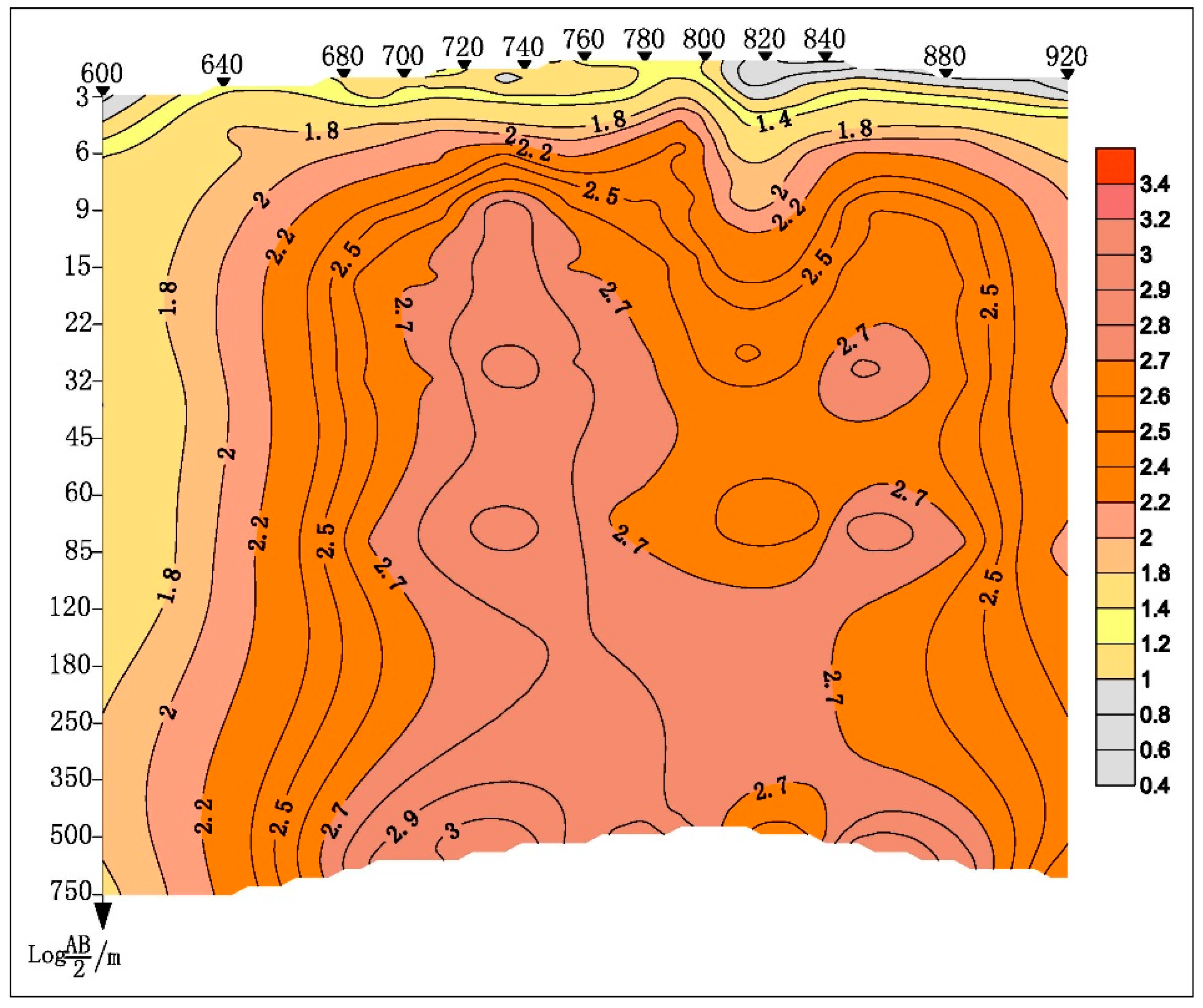
It can be seen from the apparent polarizability section of 2200 line IP sounding (Figure 9) that there was an obvious high value area of apparent polarizability near 740 points in this section. This high value area was narrow in the upper part and wide in the lower part. The highest value was greater than 3%, and it corresponded to the middle resistance area of apparent resistivity of electrical sounding. On the apparent polarizability section of 2200 line IP sounding, there was a local high value area of apparent polarizability in the deep part of the high background area near 860 points, the highest value of apparent polarizability was more than 2.8%, and the deep high value area was connected with the high value area of apparent polarizability near 740 points.

The measured apparent resistivity pseudo section reflects the relationship between the measured field and the measured pole distance. Inversion converts the measured pole distance into depth through mathematical operations and intuitively reflects the spatial position and shape of the field source. The abnormal body in reverse performance must have corresponding information displayed in its actual cross-section [19].

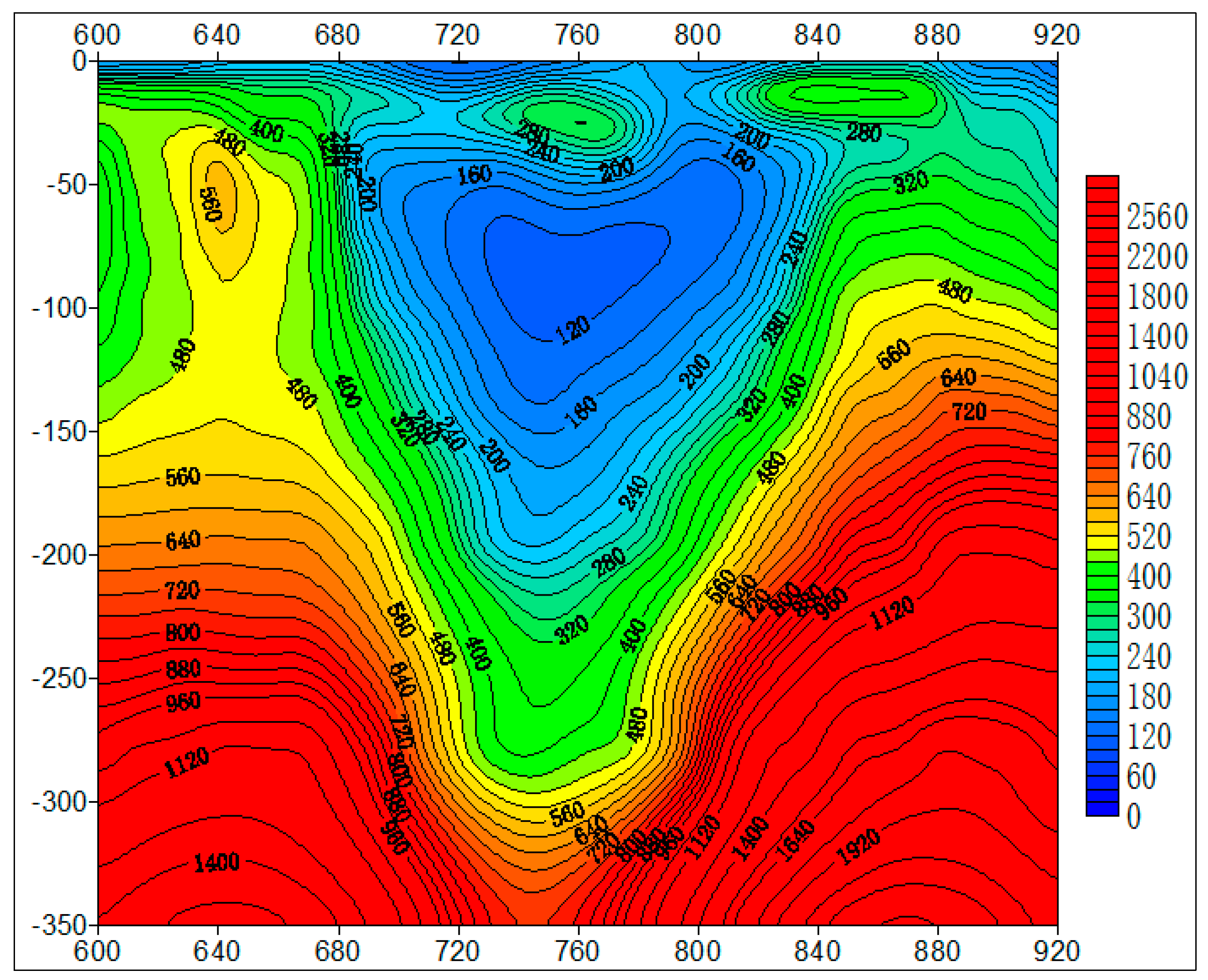
The inversion results of the sounding data of this profile are shown in Figure 10 and Figure 11. It can be seen from the figure that the horizontal and vertical variation characteristics of the apparent resistivity and apparent polarizability obtained after inversion are basically consistent with the aforementioned apparent resistivity and apparent polarizability. It can be seen from Figure 10 that the shallow layer of this section was a low resistivity layer, with resistivity less than 120 Ω⋅m, which should be a reflection of Quaternary sediments or weathered trachyte of different degrees, and the thickness of this layer was approximately 10 m. The resistivity of the underlying medium resistivity layer was between 120 Ω·m and 560 Ω·m, which should be caused by the unweathered trachyte. The thickness of trachyte gradually decreased from southwest to northeast, and gradually thinned from approximately 250 m at 600 points to about 170 m near 920 points. The resistivity of the high resistivity layer below this layer was more than 560 Ω·m, which might be granite porphyry with good integrity. 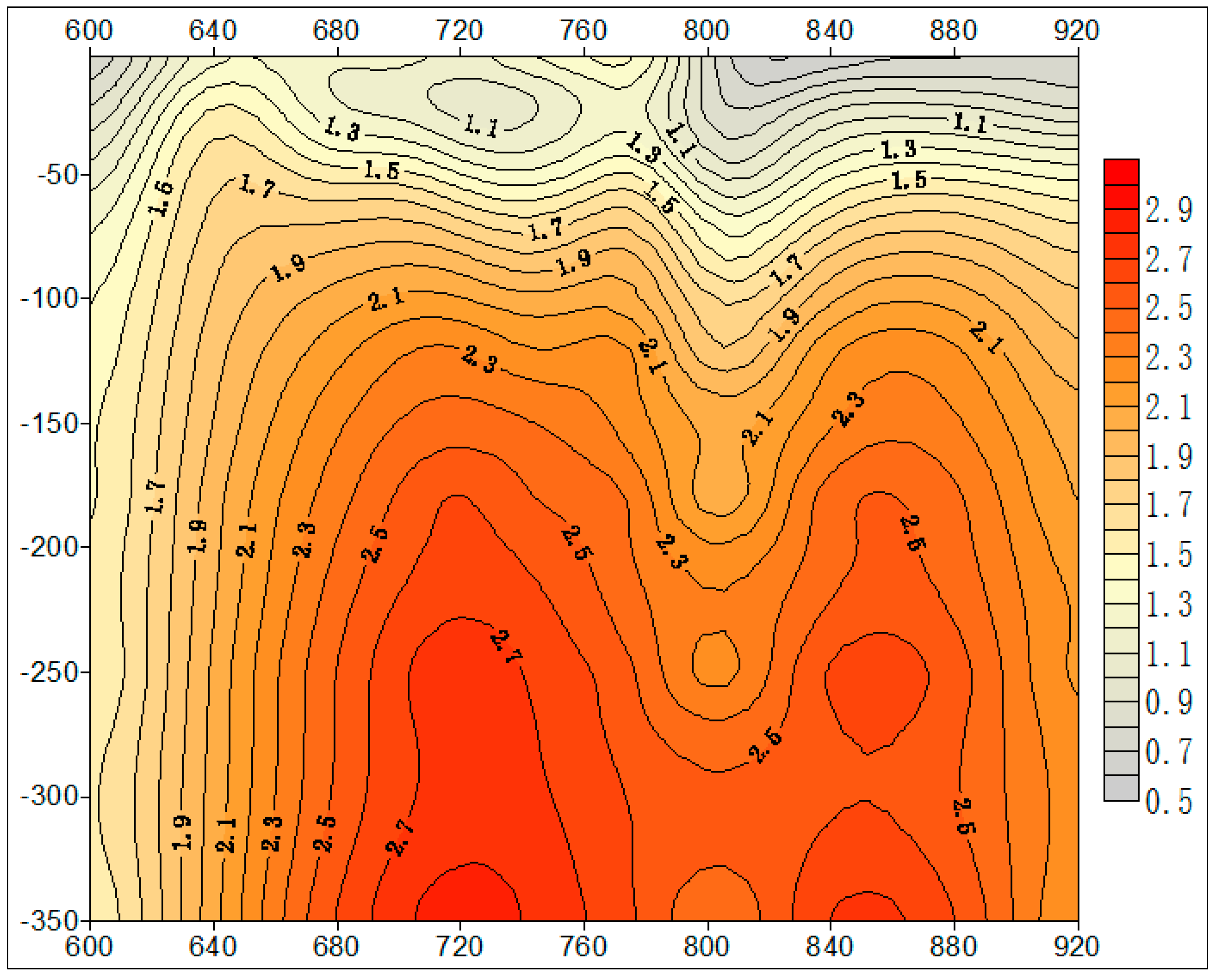It can be seen from Figure 10 that the apparent polarizability anomaly after inversion was significantly narrowed and the deep part showed two abnormal areas with high apparent polarizability, with the abnormal center at 700 and 850 points, respectively. It was speculated that the two polarizability anomalies were caused by mineralized alteration zones. It was speculated that the alteration zone near 700 points was a nearly vertical plate with a slight northeastern dip, its width was approximately 60 m, and its top buried depth was approximately 100 m. The alteration zone near 850 points was a nearly vertical plate with a slight southeast dip, its width was approximately 20 m, and its top surface was buried at approximately 120 m. The mineralized alteration zone might extend into the internal contact zone of granite porphyry, with a depth of approximately 350 m.

The geophysical results showed that from 660/100 points in the northwest of the work area to 900/2900 points in the southeast of the work area along the near southeast direction, it was an obvious low value zone of apparent resistivity, in which many local low value anomalies of apparent resistivity were distributed in beads. The scale of local anomaly varies, and the extension direction of its long axis was completely consistent with the distribution direction of the low value zone. The above low apparent resistivity zone was speculated to be a fault zone with a large extension length in the area. This fault zone showed different apparent resistivity characteristics in different sections, which might be caused by the different scale and depth of the fault zone and the thickness of the Quaternary overburden.

The abnormal metal factor reflected the distribution of tin polymetallic mineralization area in the working area. JS1, JS4, JS5, JS7, and JS9 showed the most intense tin polymetallic mineralization in the area, which had the prospect of finding shallow-buried and large-scale tin polymetallic ore bodies. The apparent metal factor had good similarity with the abnormal characteristics of the apparent resistivity and apparent polarizability. According to the electrical characteristics of rocks and ores, both polymetallic ores and tungsten mineralized quartzite in this area had high polarizability. It was speculated that this anomaly was caused by the mineralized alteration zone, which had good geological prospecting prospects.

The purpose of the inversion is to guide people’s understanding of deep geological laws by observing the geophysical characteristics of the objects. Otherwise, the proved geological phenomena can also evaluate the reliability of the inversion results. Combined with drilling verification, there is a good spatial correspondence between the abnormal polarizability region and the ore position. The abnormal excitation formed by multiple layers of ore bodies is highly consistent with the production of ore bodies, thus verifying the reliability of the inversion.

8. Conclusions

In this study, we put forward a set of induced polarization analysis strategies to extract and interpret the geophysical information of deep minerals, taking a tin polymetallic mine as an example. This strategy can provide a reliable basis for rapid development of deep geological prospecting. Obtaining IP information with low resistivity and high polarization in the abnormal area can reflect the spatial occurrence of deep mineral structures to a certain extent and can be used as an indirect clue for prospecting. At the same time, through systematic verification, the metal ore (mineralized) body and altered rock in the mining area are compared with the IP information in the abnormal area. The obtained abnormal area is consistent with the known altered mineralized geological body and has a strong correlation, which shows that the exploration results can objectively reflect the deep geology and mineral occurrence in the mining area, thus providing a more sufficient basis for guiding the engineering verification.