The Environmental Kuznets Curve Hypothesis for Colombia: Impact of Economic Development on Greenhouse Gas Emissions and Ecological Footprint

Abstract

Climate change has become a significant concern for developing countries given the risk that it poses to energy and food independence, and to general productivity. Despite having an energy system with low carbon intensity when compared to other Latin American countries, Colombia is already facing climate change impacts and requires urgent efforts to mitigate them. As a developing country, the challenge is bigger as policies for economic growth should be in line with the global commitment of reducing greenhouse gas emissions. With the aim of contributing to the design of climate policies by using data driven methodologies and scientific evidence, this study assesses the impact of economic development on the environment by examining the validity of the environmental Kuznets curve hypothesis for Colombia. Statistically validated and stable autoregressive distributed lag models are estimated for three different environmental indicators: carbon dioxide emissions, methane emissions, and the ecological footprint. Moreover, the effects of other variables such as urbanization, foreign direct investment, the value added by the agricultural and industrial sectors, and energy use are analyzed with dynamic simulations. To the best of our knowledge, there are no reports of EKC estimation using these variables in statistically validated models for Colombia; thus, this paper adds to the scientific evidence of the EKC hypothesis in developing countries. Empirical evidence supports a long-run equilibrium relationship among investigated variables and the existence of an inverted U-shaped EKC relationship between gross domestic product (GDP) and methane emissions, and GDP and the ecological footprint. The results of this paper show that shifting to renewable energy sources and leveraging the use of cleaner technologies in agricultural and industrial sectors are key factors for economic growth without harming the environment, which has important scientific value because of its evidence-based approach for public policy making in developing countries, particularly Colombia.

1. Introduction

Climate change mitigation has become a significant concern for both developed and developing countries. The increase in environmental degradation, greenhouse gas (GHG) emissions, and global warming is mainly a result of human activities, and the potential consequences are so dreadful that researchers, leaders, and politicians around the world have begun to prioritize efforts with regard to investigating climate change causes and designing appropriate policies to mitigate its impacts. As international cooperation and global solutions are required, world leaders from almost 200 countries met in November 2021 at the United Nations Climate Change Conference (COP26) and made enhanced commitments to accelerate actions towards the goals of the Paris Agreement, such as limiting the rise of mean global temperature to 1.5 °C.

Reaching global net-zero carbon dioxide (CO₂) emissions, phasing down coal power, halting and reversing deforestation, switching to electric vehicles, and reducing methane (CH₄) emissions are among the main commitments settled in the Glasgow Climate Pact, which resulted from COP26 [1]. However, designing policies and actions to contribute to these global objectives represents an important challenge, especially for developing countries, because the majority of them are in desperate need of economic development to improve the life quality of their people and address the consequences of global warming that they are already facing, such as resource scarcity.

In order to appropriately design strategies and policies to meet these ambitious pledges, it is necessary to understand the specific economic and environmental situation of each country as economic development and environmental degradation are expected to be related and a balance must be achieved to reach sustainable development. Providing important new evidence on how economic activities associated with the development of countries affects climate change is essential to make policies that permit the improvement of the quality of life of citizens with sustainable commitments. This is especially true for developing countries, whose economic progress must be made in an era in which environmental restrictions require different methods of industrialization. That is the case of Latin American countries, in which there is still a strong necessity for transforming their economies while improving institutional and public services and reducing inequality [2].

We concentrate our study in Colombia, as a country that is transitioning in Latin America, with constant rates of economic growth during the last decades. Although Colombian GHG emissions only represent 0.4% of global emissions, according to 2018 data from the World Bank, the country is not exempt from the climate change mitigation discussion [3]. In fact, the United States National Intelligence Council has identified Colombia, along with other 10 countries from Asia, Central America, and the Caribbean, as one of the countries of great concern due to the threat of climate change as it is considered highly vulnerable to its physical effects and lacks the capacity to adapt [4]. Because of this, the Colombian government recognized the need for actions in the country and made ambitious commitments at COP26: they declared 30% of its territory a protected area and planted 180 million trees by 2022; they will achieve a 51% reduction in GHG emissions by 2030, and reach carbon neutrality by 2050. Furthermore, Colombia joined the alliance proposed by the government of the United States of reducing methane emissions by 30% from 2020 levels by the end of the decade.

The aim of this study is to assess the nexus between economic development and environmental degradation in Colombia by testing the validity of the environmental Kuznets curve (EKC) hypothesis, including macroeconomic variables that may also affect the environment, such as urbanization; the value added by the agricultural and industrial sectors; energy consumption; and foreign direct investment. The EKC hypothesis posits that pollution emissions increase and environmental quality declines when a country or region is in the early stages of economic growth, but beyond some level of income per capita, the situation changes so that higher income levels lead to increased environmental awareness, the enforcement of environmental regulations, cleaner technologies, and higher environmental expenditures, resulting in a gradual decline in the level of pollution and environmental degradation [5,6,7].

Estimating and analyzing the EKC has become the main approach in the energy and economic literature to understand development impacts on the environment and provide recommendations on public policy making accordingly. There is a wide range of literature investigating the validity of the EKC hypothesis for different countries and periods, and considering multiple environmental indicators and macroeconomic variables [8,9]. Nonetheless, there is a lack of research in the case of Latin American and Caribbean countries. Particularly in Colombia, the few existing studies of the relationship between economic development and environmental degradation in the country are focused on carbon dioxide emissions as an environmental indicator, failing to consider other relevant factors related to the environment.

This paper contributes to the existing literature by trying to fill the cited gap by estimating and studying the potential relations between gross domestic product (GDP) per capita and three different indicators of environmental degradation: carbon dioxide emissions, methane emissions, and the ecological footprint. First, carbon dioxide emissions are the main focus in global climate change mitigation, which makes it essential for environmental degradation analysis. From the few existing studies of the carbon dioxide emissions relationship with the economic development for the Colombian case, there are mixed results, and in most cases these are not supported by statistically validated models. Henceforth, we seek to provide new scientific evidence to better understand this nexus and contribute to the debate on carbon reduction and the design of environmental policies, for Colombia.

Moreover, we extend the analysis by studying methane and the ecological footprint. According to data retrieved from the climate analysis indicators tool (CAIT) [10], the level of methane emissions in Colombia is almost the same as carbon dioxide emissions and has been increasing over the years, with the agricultural sector being mainly responsible. Assessing the economic development impact on methane emissions is therefore especially relevant for Colombia considering that this gas has a 100-year warming potential 28 times larger than CO₂ [11]. Lastly, the ecological footprint is appropriate for measuring environmental degradation as it converts the impact sources (electricity, food, water, materials) and waste generation (such as carbon dioxide emissions) into the equivalent biologically productive land required to produce or absorb these impacts [12]. Ecological footprint results have been used as an indicator of environmental degradation to investigate the EKC hypothesis by some empirical studies [9,13,14]. However, to the best of our knowledge, there are no reports of EKC estimation for the ecological footprint in Colombia, although they may be a powerful indicator to understand environmental impact and sustainable resource use in the country rather than only focusing on air pollutant accumulation.

To estimate a model for each environmental degradation indicator, we use the autoregressive distributed lag (ARDL) bound testing procedure by Pesaran, Shin, and Smith [15]. This methodology allows us to test if cointegration exists, has strong small sample properties, and provides unbiased estimates of the long-run model and valid t-statistics even in the presence of endogeneity [15,16]. Furthermore, we use stochastic simulations to easily and properly interpret the causal relationships between the variables and make substantive statistical inference from our ARDL models, contributing to better understanding the impact of related variables.

The study is structured as follows: Section 2 presents the literature addressing the EKC hypothesis, the Colombian environmental context, and the contribution of our study; Section 3 focuses on data description and the econometric methodology; Section 4 reports the empirical results and discussion; and Section 5 concludes the study.

2. Literature Review

The Kuznets curve hypothesis has its origin in the work of Simon Kuznets in 1955, who found an inverted-U shaped relationship between per capita income and income inequality, implying that the initial stage of income growth is characterized by unequal income distribution; however, there is a turning point in economic growth where income distribution starts moving towards equality [17]. This initial contribution was extended to the environmental field when [5] investigated the North American Free Trade Agreement (NAFTA) and also found an inverted-U shaped relationship between air pollutants (sulfur dioxide and smoke) and income per capita. Then, with the work of [6], where the hypothesis was validated by the World Bank, it became a controversial topic in the scientific community as it was stated that the view that greater economic activity inevitably hurts the environment is mistakenly based on static assumptions about technology, tastes, and environmental investments [18].

The expression ‘environmental Kuznets curve hypothesis’ appeared for the first time in the literature in 1993 when Panayotou studied the economic growth effect on air and land [7]. This position has been expounded even more forcefully by authors such as Beckerman [19], who stated that the best and probably only way for a country to attain a decent environment is to become rich, whereas others such as Van Alstine and Neumayer [20] clarify that economic growth by itself will most likely not be the solution to environmental degradation as some developing countries will not reach the turning point for decades to come.

From those first contributions in the 1990s, the EKC has become the main framework in the energy economic literature to study the relationship between environmental degradation, economic development, and other variables, such as energy consumption. Due to the assertiveness of the policies that emanate from EKC estimation and analysis, there is a vast number of studies in economic literature that have focused on the empirical and theoretical investigation of its validity providing a varied mixture of results as they depend on the econometric models, the variables included, the environmental degradation indicators employed, and the sample of countries and periods chosen to examine the relationship [8,9].

Some authors focus their studies on individual countries, for example, Kenya [21], USA [22], Pakistan [16], South Africa [23], and China [24], whereas others investigate the EKC for a group of countries from a specific region or with similar characteristics, such as Sub-Saharan African countries [25], the top five emitters of greenhouse gas emissions from fuel combustion in developing countries [26], 15 Middle East and North African (MENA) countries [9], 36 high-income countries [27], and 16 European Union countries [28]. Depending on the latter, econometric techniques employed vary from vector autoregression (VAR) models, Johansen cointegration approaches, ARDL bounds technique, and Granger causality tests, in the case of individual countries, to the panel cointegration approach, dynamic ordinary least squares regression (DOLS), fully modified ordinary least squares regression (FMOLS), and the panel-vector error-correction model (VECM), among others, for studies considering a group of countries.

In addition to the sample of countries and the estimation method employed, the turning point in income levels varies depending on the selected indicator of environmental degradation. As reviewed by Sarkodie and Ozturk [8], the majority of studies are based on carbon dioxide emissions due to its signifcant impact on GHG emissions (carbon dioxide, nitrous oxide, methane, perfluorocarbons, sulfur hexafluoride, and hydrofluorocarbons), while other atmospheric indicators such as sulfur dioxide or air pollutants (PM₁₀, PM_2.5) concentration are less considered [29]. Land indicators, such as fertilizer consumption [30] or deforestation [31]; freshwater indicators, such as biological oxygen demand (BOD) [32] or water pollution [33]; and biodiversity indicators [34] have also been used as environmental degradation proxies for estimating the EKC.

The variables included in the estimated equation also affect the results. Bias from omitted variables, integrated variables, spurious regression, and the identification of time effects are the main econometric problems when estimating the EKC [18]. Some authors have tested the basic equation, only including income per capita and its squared form in the model, but others have augmented this equation by including the cubic form of income per capita and other variables that may affect the environmental indicator, such as urbanization, financial development, foreign direct investments, and energy consumption. Due to the differences exposed, results from studies vary from the validation of the EKC hypothesis to finding a linear or N-shaped relationship. As results cannot be generalized, it is necessary to study the specific Colombian case in order to reach our goal of understanding the economic and environmental nexus in the country to provide recommendations for policy design.

As mentioned before, despite the wide range of literature investigating the EKC hypothesis, there is a lack of research in the case of Colombia and, in general, Latin American and Caribbean countries. There are few authors that have estimated EKC model using panel data from a group of countries of the region, including Colombia [35,36]. Meanwhile, only six studies were identified that address relationships from the EKC hypothesis specifically in Colombia, and these did not contain conclusive evidence as mixed results were obtained. Firstly, Vásquez and Garcia (2003) used solid waste, GDP per capita, and a technologically advanced indicator for the Aburrá Valley Metropolitan Area using OLS, resulting in a model with adjusted R-squared of 90% but not conclusive results about EKC [37]. Then, Correa, Vasco, and Pérez (2005) considered carbon dioxide emissions, sulfure dioxide emissions, biological oxygen demand, GDP per capita, the GINI index, political freedom, and the literacy rate using OLS, and the results showed that Colombia is on the upward slope of the EKC, meaning that economic growth is worsening environmental quality [38]. Afterwards, Ruiz-Agudelo et al. (2019) utilized the endangered species total number, GDP per capita, the GINI index, the environmental performance index, and the literacy rate using OLS, and the results showed that the EKC hypothesis is not met for Colombia [34]. Additionally, Sosa and Navarro (2020) utilized carbon dioxide emissions, GDP per capita, energy consumption, urbanization, and economic complexity using the ANFIS model, FMOLS, and DOLS and did not find conclusive results for the EKC hypothesis [39]. Finally, Laverde-Rojas et al. (2021) considered carbon dioxide emissions, GDP per capita, electric power consumption, foreign direct investment, urban population, exports and imports, and economic complexity index using VECM and found that the EKC hypothesis is not valid for Colombia and there is no evidence that improvements in economic complexity have positive effects on reducing pollution levels [40].

Given this inconclusiveness and the fact that some of these results came from not statistically validated models, we aim to contribute to the literature and provide reliable results for policy making by implementing statistically validated ARDL models to test the EKC hypothesis for Colombia not only considering carbon dioxide emissions as environmental indicator but also methane emissions and the ecological footprint.

3. Materials and Methods

In order to select the environmental indicators and macroeconomic variables to consider in our study, we started by researching the Colombian economic and environmental context and making an exploratory data analysis of climate-, pollution-, and economic-related time series available on public sources [3,10,41], and Our World in Data [42,43]. From this analysis, we ended by selecting the variables listed in

Table 1. Variables definition.

Variable Name	Code	Period Available	Unit of Measurement
Environmental degradation indicators
Carbon dioxide (CO2) emissions per capita	CO2	1960–2018	metric tons (t)
Ecological footprint per capita	EF	1961–2018	global hectares (gha)
Methane (CH4) emissions per capita	CH4	1970–2018	metric tons (t)
Independent variables
Agriculture, forestry, and fishing, value added per capita	AFF	1965–2020	constant 2015 US$
Foreign direct investment, net inflows per capita	FDI	1970–2019	constant 2015 US$
GDP per capita	GDP	1960–2020	constant 2015 US$
Industry, value added per capita	IND	1965–2020	constant 2015 US$
Non-renewable energy use per capita	NREU	1965–2019	kilowatts per hour (kWh)
Renewable energy use per capita	REU	1965–2019	kilowatts per hour (kWh)
Urban population ratio	URB	1960–2020	–

.

3.1. Environmental Degradation Indicators

We selected three environmental degradation indicators, aiming to estimate a model and study the nexus with economic development for each of them. Metric tons of CO₂ and CH₄ emissions per capita were retrieved from the world development indicators (WDI) [3]. In Figure 1, it can be seen that CO₂ emissions per capita have been historically increasing with few exceptions, such as the beginnings of the 21st century, probably as a response to the Colombian financial crisis in 1999. Meanwhile, there is no marked behavior of CH₄ emissions per capita, which have been changing between 1.48 and 1.75 and, at least until 2012, were historically higher than CO₂ emissions. Although CH₄ emissions per capita decreased in the recent years, Figure 1 shows us the similarity on the level of emissions of both greenhouse gases and reinforces the relevance of studying them both as they represent major threats to the environment.

On the other hand, ecological footprint (EF) per capita series was extracted from the global footprint network open data platform [41]. EF is measured in global hectares (gha), which is equivalent to biologically productive hectares given the average world biological productivity for a given year. Figure 2 shows the series and allows us to observe that, at least according to this indicator, the environmental conditions are actually improving in Colombia as the per capita demand of natural resources is decreasing.

3.2. Economic Development Indicator

Regarding the economic development indicator, we selected the GDP per capita as in most of the studies on the EKC framework. We retrieved the data from the WDI in constant 2015 USD to prevent the influence of price inflation [3]. The series has been historically increasing, except in 1999, when the GDP per capita fell by 5.7% due to Colombian financial crisis. Owing to the Great Recession of 2008, the GDP per capita only changed by 0.02% from 2007 to 2009. However, from 2009 to 2019 there was important economic growth in the country, reflected by a 27.99% increase in GDP per capita, with a mean annual rate of 2.51%.

3.3. Additional Macroeconomic Variables

Energy consumption is strongly believed to be associated with environmental degradation and hence is also included in our study. As most countries generate their energy primarily from fossil fuels (coal, oil, and gas), it is reasonable to believe that the increase in energy consumption, at least from non-renewable sources, will directly result in more carbon dioxide emissions, thereby harming the environment. On the contrary, increasing the generation of energy from renewable sources is seen as one of the best ways of mitigating climate change. Aiming to obtain more accurate models and to empirically confirm these effects, we include in our study both renewable and non-renewable energy consumption per capita in kilowatts per hour (kWh), which were retrieved from Our World in Data, based on BP & Shift Data Portal [43]. On average, from 1970 to 2018, 74.4% of the total energy used came from fossil fuels. Although the renewable energy use per capita has been increasing periodically and the proportion of energy used that came from these sources increased 14 percent points from 1970 to 2018, the differences in growth rates when compared to non-renewable sources is notorious. From 2005 to 2018, non-renewable energy use per capita increased by 49.29%, whereas renewable energy use raised only by 17.65%.

In addition to energy use, we also include two indicators of agricultural and industrial importance in Colombia as they are the first and third sector contributing to GHG emissions in the country, respectively. Specifically, aiming to validate if there is a relationship between these activities and environmental degradation, we include the value added by agriculture and industry. Value added is the net output of a sector after adding up all of the outputs and subtracting intermediate inputs [3]. Agriculture and industry value-added series were retrieved from the WDI and are measured in constant 2015 USD$, and the variables are expressed in per capita values. We can evidence from

Table 2. Summary statistics.

Variable	Mean	Std Deviation	Median	Minimum	Maximum	Skew	Kurtosis
CO2	1.54	0.12	1.56	1.32	1.74	−0.28	−1.15
CH4	1.61	0.08	1.61	1.48	1.75	−0.08	−1.25
EF	2.08	0.14	2.10	1.81	2.33	−0.08	−1.23
AFF	301.73	38.47	303.92	226.63	389.45	0.23	−0.08
FDI	103.12	94.24	68.44	4.60	309.48	0.76	−0.82
GDP	4019.90	1109.67	3911.57	2345.81	6271.88	0.64	−0.55
IND	1246.03	270.43	1243.95	764.83	1771.37	0.39	−0.67
NREU	5836.66	801.59	5669.89	4535.95	7861.42	0.87	0.02
REU	2059.67	630.36	2303.56	782.73	3040.81	−0.60	−0.86
URB	0.70	0.07	0.71	0.57	0.81	−0.34	−1.03

that industry has been more important than the agricultural sector in Colombia during the sample period. Between 1970 and 2018, the average value added per capita of the industrial sector was 1246.03 USD$, whereas the average value added per capita of the agricultural sector was only 301.73 USD$. Even though both series have increasing behavior, the growth rates are considerably different (120.47% for industry versus 69.12% for agriculture between 1970 and 2018). Transport is the second most important sector for GHG emissions, but it is not included as there are not available data on reliable sources.

Another variable that is frequently used in the EKC framework as it directly influences GDP increments is the net inflows from foreign direct investment (FDI). There are two contrasting hypothesis in the literature. Some believe that through foreign direct investments developed countries help developing countries by creating jobs and promoting innovation, research, and development, and the use of cleaner and modern technologies, thus having a positive effect on the environment. Contrary to these arguments, others believe that an increase in FDI may raise manufacturing activities and lead to higher pollution levels. Especially when environmental regulations are weak, companies from developed countries are tempted to shift their industries to developing countries [26]. The foreign direct investment series was also extracted from the WDI in constant 2015 USD$ and divided by the population to be expressed in per capita values. Although there is not a marked behavior in the time series, changing considerably year by year, we can state that FDI has experienced important growth within the last 20 years, especially from 2004 to 2005 and from 2010 to 2011 (173.18% and 106.42% respectively).

As can be noted, all of the analyzed variables are expressed in per capita values, taking into account population growth. However, it is interesting to consider how the urban population is growing as urbanization may be an important determinant of environmental degradation. Regarding this effect, there are also two contrasting theories. The first one, known as the ecological modernization theory, argues that urbanization leads to modernization and social transformations, contributing to the development of sustainable institutions, policies, and technologies that help improve environmental quality. By contrast, others believe that urbanization inevitably means an increase in the demand of food, electricity, gasoline, gas, and other resources and hence leads to more industrial processes, more GHG emissions, and worse environmental quality [9,44]. Urban and total population series were available on the WDI database, and we simply calculated the ratio between them. We noticed that urban population ratio has been monotonically increasing, reaching almost 81% by 2018.

The summary statistics of all of the selected variables are presented in Table 2. These statistics were calculated for the period between 1970 and 2018 as we have the information of each variable for each year within that period.

To examine the nexus between the variables selected, testing the presence of cointegration and contrasting the validity of the EKC hypothesis, we employ the ARDL modelling approach proposed by Pesaran, Shin, and Smith [15], which, unlike other econometric techniques, does not require variables to be integrated in the same order and allows us to include I(0) and I(1) variables indistinctly, even if the underlying regressors are mutually cointegrated [45]. This is a great advantage given that most macroeconomic variables are proved to be integrated with one of these orders. Furthermore, this method has shown robust outcomes for small sample sizes and the unbiased estimation of the long-run model even in the presence of endogeneity [21,46]. Given these advantages, for each environmental indicator (CO₂, CH₄ and EF), we estimate an ARDL model, where we express all of the variables in their natural logarithms aiming for a more stable data variance.

3.4. ARDL Estimation, Validation, and Model Selection

First, we perform unit root tests in order to check that the regressors are not of order I(2) or more, and that the dependent variable of each model is I(1). For this purpose, augmented Dickey Fuller (ADF) and Phillips Perron (PP) tests are used. For variables in levels and after taking first differences, we contrast the null hypothesis of a unit root in the series against the alternative of stationarity (see [47] for further details). Once ensured that the dependent variable is I(1) and the regressors are I(0) or I(1), ARDL models are estimated aiming to find the best specification. We start by estimating two models regressing each environmental degradation indicator on the independent variables described in Table 1, the first one with trend (adding the term ${\alpha }_{1}t$) and another without trend (1).

$$lnED{I}_t={\alpha }_0+\sum _{i=1}^p{\varphi }_{i}lnED{I}_{t-i}+\sum _{i=0}^{q_1}{\beta }_{1,i}lnGD{P}_{t-i}+$$

$$\hspace{1em}\hspace{1em}\hspace{1em}\sum _{i=0}^{q_2}{\beta }_{2,i}{\left(lnGD{P}_{t-i}\right)}^2+\sum _{j=1}^k\sum _{i_j=0}^{r_j}{\lambda }_{j,i_j}ln{Z}_{j,t-i_j}+{ϵ}_t$$

(1)

Here, $EDI$ (environmental degradation indicator) is the dependent variable (either CO₂, CH₄, or EF) and $GDP$ is the series of the GDP per capita; its respective quadratic term is included to estimate the EKC. $Z_j$ corresponds to the other k regressors selected (AFF, FDI, IND, NREU, REU, and URB). For optimal lag selection, we use the Schwarz–Bayesian criterion (SBC) as it is a consistent model selection criterion, and it has been shown by empirical testing that it performs better than other criterion such as the Akaike information (AIC). Moreover, as we have a small sample size but a considerable number of regressors, SBC provides a suitable lag length to preserve freedom degrees as it suggests the minimum of lags relevant to the model [2,45].

Since the ARDL approach may be sensitive to the specification of the model, and the existence of structural breaks, it is important to check in detail all assumptions to provide robust results. In that sense, each of the models are statistically validated by performing diagnostic and stability tests, which is essential to prevent spurious regression or biased and inconsistent estimates. First, we perform Jarque-Bera (JB) test for residual normality [48], which evaluates if the skewness and kurtosis of the data match that of a normal distribution by using the first four estimates of the corresponding central moments. This statistic asymptotically has a chi-squared distribution, and the null hypothesis establishes that the data fits a normal distribution. Then, we perform the Breusch–Pagan–Godfrey (BP) test for heteroskedasticity [49], which is derived from the Lagrange multiplier test principle, and its null hypothesis establishes the presence of homoskedasticity. Afterwards, we perform the Breusch–Godfrey–Lagrange multiplier (BG-LM) test for serial correlation [50], which is also derived from the Lagrange multiplier test principle, and its null hypothesis establishes the absence of serial correlation. Then, we perform the Ramsey RESET test for the functional form misspecification [51], which uses a F statistic to test the need of incorporating nonlinear terms in the regression model, and its null hypothesis establishes the absence of said terms. Finally, we perform the Cumulative Sum (CUSUM) and CUSUM of Squares (CUSUMSQ) tests [52] for structural change by using sequential analysis and establishing under the null hypothesis constancy in the time series, i.e., no structural change.

The ARDL-bounds cointegration test relies on the assumption of serially uncorrelated errors; therefore, it must be ensured that the residuals from our ARDL estimation are white noise [53,54]. Based on the results of the diagnostics test and on fit metrics such as AIC, SBC, and adjusted R squared, we select the best model for each dependent variable, that is, we define if a linear trend should be included or not. However, aiming to improve our models, we check the significance of the regressors and perform Wald’s redundant variables test. By this, we define the regressors that should be considered and estimate our final model, which is also statistically validated with the diagnostic and stability tests previously mentioned.

Although model (1) represents the long run relations among variables in levels, the estimation of the real dynamic effects requires further investigation if a cointegrated relation exists. Through a simple linear transformation, the model presented in Equation (1) can be rewritten as (2) for the case in which there is no trend (otherwise, the term ${\delta }_{1}t$ is included).

$$\Delta lnED{I}_t={\delta }_0+{\theta }_{0}lnED{I}_{t-1}+{\theta }_{1}lnGD{P}_{t-1}+{\theta }_2{\left(lnGD{P}_{t-1}\right)}^2+$$

$$\hspace{1em}\hspace{1em}\sum _{i=3}^{k+2}{\theta }_{i}ln{Z}_{i-2,t-1}\sum _{i=1}^{p-1}{\pi }_{0,i}\Delta lnED{I}_{t-i}+\sum _{i=0}^{q_1-1}{\pi }_{1,i}\Delta lnGD{P}_{t-i}+$$

$$\hspace{1em}\hspace{1em}\hspace{1em}\hspace{1em}\sum _{i=0}^{q_2-1}{\pi }_{2,i}\Delta {\left(lnGD{P}_{t-i}\right)}^2+\sum _{j=3}^{k+2}\sum _{i_j=0}^{r_j-1}{\pi }_{j,i_j}\Delta ln{Z}_{j-2,t-i_j}+{\nu }_t$$

(2)

Here, the terms from ${\theta }_1$ to ${\theta }_{k+2}$ describe the long-run dynamics of these variables, whereas the terms associated with the differentiated variables (i.e., with coefficients $\pi$) describe the short-run dynamics.

Then, the ARDL F-bounds test is performed, in which the null hypothesis is $H_0:{\theta }_0={\theta }_1={\theta }_2={\theta }_3=\dots ={\theta }_{k+2}=0$ (no cointegration), while the alternative is that at least one of these coefficients is different from 0. To conclude, we compare the F-Wald statistic with the critical values, either from the asymptotic case [15] or considering the actual sample size [55]. The critical values I(0) and I(1) are the lower and upper bounds, and there are three cases: if the F statistic is lower than the I(0) bound value, then the null hypothesis is not rejected, and we conclude there is no cointegration; if the F statistic is greater than the I(1) bound value, we reject $H_0$, and there is evidence to conclude that variables are cointegrated; and, finally, if the F is between the critical values, the test is inconclusive. In order to provide robustness to our results, we also used the t-Bounds test, to rule out nonsensical cointegration. In this case, the null hypothesis is that the coefficient on the lagged dependent variable (in levels) is equal to zero, i.e., $H_0:{\theta }_0=0$, against $H_1:{\theta }_0<0.$ There are also I(0) and I(1) bound values, to which we compare the t-statistic. If we concluded that there is cointegration from the F-bounds test, the absolute value of the t-statistic should be greater than the absolute value of I(1).

If the existence of a cointegration relationship is concluded, we proceed to analyze the short-run dynamics by defining the respective error correction model (ECM):

$$\hspace{1em}\hspace{1em}\Delta lnED{I}_t={\delta }_0+\sum _{i=1}^{p-1}{\pi }_{0,i}\Delta lnED{I}_{t-i}+\sum _{i=0}^{q_1-1}{\pi }_{1,i}\Delta lnGD{P}_{t-i}+$$

$$\sum _{i=0}^{q_2-1}{\pi }_{2,i}\Delta {\left(lnGD{P}_{t-i}\right)}^2+\sum _{j=3}^{k+2}\sum _{i_j=0}^{r_j-1}{\pi }_{j,i_j}\Delta ln{Z}_{j-2,t-i_j}+\gamma EC{T}_{t-1}+{\nu }_t$$

(3)

where $EC{T}_{t-1}$ is the error correction term lagged one period and the coefficient $\gamma$ is the speed of adjustment, which measures how fast the variables return to long-run equilibrium. This coefficient must be negative and highly significant.

3.5. Dynamic Simulations

Even though we can directly interpret and make inferences from the estimated long-run and short-run coefficients and their standard errors, it may be difficult to discern the effects of a change in the regressors on the environmental indicators given that multiple lags, differences, or lagged differences can be included in our ARDL models [54]. Therefore, using the methodology described in [56], we implement dynamic stochastic simulations to complement our analysis. Specifically, the coefficients are simulated from a multivariate normal distribution given the mean and variance of the estimator. For each regressor, a shock of 10% is forced to obtain a plot of its impact on the dependent variable in the following periods, allowing us to observe and interpret the effects more precisely.

3.6. EKC Validation

Finally, to fulfill the objective of validating the existence of the EKC in Colombia, we adopted the Utest approach proposed by Lind and Mehlum [57]. In most empirical works, researchers usually conclude that there is a U-shaped (or an inverse U-shaped) relationship if the regressor and its quadratic term are significant and have the right signs. However, to avoid misleading outcomes, we also check if the turning point is within the data range and then contrast the null hypothesis that the relationship between GDP and each environmental indicator is increasing at low values and decreasing at high values within the sample interval (there is an inverse U-shape), against the alternative of a U-shaped or monotone relationship. Moreover, we end our methodology by estimating a confidence interval for the turning point using the method proposed by [58].

4. Results and Discussion

4.1. ARDL Estimation, Validation, and Final Model Selection

After selecting our variables and applying a logarithmic transformation for each of them, our econometric empirical analysis starts by testing the stationarity properties of the variables. Specifically, we perform ADF and PP tests for each variable. For both unit root tests, the different possible cases of test equation are considered: including a deterministic trend and an intercept, considering just an intercept but no trend, and omitting both (just for ADF). We select the number of lags for the ADF test according to the Schwarz–Bayesian Criterion (SBC) with a maximum of four lags considered, whereas for the PP test we set the number of lags to the integer value 12(T/100)^1/4 proposed by [59]. From the test statistics presented in

Table 3. Unit root tests statistics.

	ADF Levels			PP Levels		ADF 1st Diff			PP 1st Diff
Variable	Trend	Drift	None	Trend	Drift	Trend	Drift	None	Trend	Drift
lnCO2	−2.18	−2.20	−0.20	−2.82	−2.88	−4.71 **	−4.76 **	−4.80 **	−8.63 **	−8.71 **
lnCH4	−2.36	−2.39	−0.32	−2.31	−2.41	−4.95 **	−4.95 **	−5.00 **	−8.39 **	−8.39 **
lnEF	−1.21	−1.50	−0.05	−1.8	−1.96	−7.08 **	−7.03 **	−7.10 **	−7.72 **	−7.39 **
lnAFF	−2.64	−2.74	0.18	−2.16	−2.36	−5.62 **	−5.62 **	−5.66 **	−7.61 **	−7.30 **
lnFDI	−1.80	−1.92	−0.38	−1.66	−1.83	−5.47 **	−5.35 **	−5.40 **	−7.72 **	−7.60 **
lnGDP	−1.93	−2.09	0.08	−1.94	−2.22	−5.29 **	−5.24 **	−5.28 **	−7.91 **	−7.66 **
lnIND	−1.97	−2.10	0.00	−2.02	−2.37	−5.17 **	−5.11 **	−5.16 **	−7.73 **	−7.43 **
lnNREU	−2.47	−2.53	0.04	−2.36	−2.47	−4.72 **	−4.74 **	−4.79 **	−8.26 **	−8.12 **
lnREU	−2.32	−2.32	0.12	−2.01	−2.34	−6.08 **	−5.98 **	−6.04 **	−8.06 **	−7.50 **
lnURB	−1.84	−1.98	−0.72	−1.74	−2.11	−5.37 **	−5.26 **	−5.30 **	−8.10 **	−7.70 **

** Null hypothesis rejected at 1% significance level.

, we can evidence that all variables are I(1).

Given the unit root tests results, we proceed to estimate, validate, and select our final ARDL model for each environmental indicator.

Table 4. CO₂ model metrics and diagnostic tests results.

Response: lnCO2	No Trend	Unrestricted Trend	Unrestricted Trend and No AFF
Lag selected	(3,0,1,1,1,1,0,0,1)	(1,0,1,1,0,1,0,0,1)	(1,–,1,1,0,1,0,0,1)
SBC	−4.0893	−4.4045	−4.4836
AIC	−4.7651	−4.9893	−5.0294
Adj R-squared	0.9365	0.9496	0.9511
Jarque-Bera	2.1289 [0.3449]	0.6201 [0.7334]	0.6451 [0.7243]
Breusch-Godfrey	4.8998 [0.0153] *	1.6906 [0.2010]	1.8811 [0.1689]
Breusch-Pagan	0.3488 [0.9850]	0.5967 [0.8481]	0.6767 [0.7711]
Ramsey RESET	2.2522 [0.1246]	2.3518 [0.1120]	2.5209 [0.0962]

Variables ordered as (lnCO₂, lnAFF, lnFDI, lnGDP, (lnGDP)², lnIND, lnNREU, lnREU, and lnURB). ‘–’ means that the variable is not included. For each diagnostic test, the statistic is presented and the number between square brackets is the p-value. * Null hypothesis rejected at 5% significance level.

reports the results for carbon dioxide emissions. The model including an intercept and all of the regressors has an adjusted R-squared of 0.9365; however, with a BG-LM statistic of 4.90 and a p-value lower than 0.05, the null hypothesis of no serial correlation of order 3 is rejected. On the other hand, a model including an unrestricted trend leads to better adjusted R-squared, AIC, and SBC, while failing to reject the null hypothesis for all of the diagnostic tests. Therefore, in this second model it is not possible to identify problems of heteroskedasticity, specification error, or serial correlation, and its residuals are normally distributed. With a p-value of 0.82, agriculture value added per capita is not a significant variable and hence is excluded from the final model. By doing so, the model improves in all its fit metrics and remains statistically valid. Furthermore, model residuals are independent and have stable parameters to make unbiased statistical inference, as is shown from the CUSUM and CUSUM of squares tests, presented in Figure 3a and Figure 4a.

Similarly,

Table 5. CH₄ model metrics and diagnostic tests results.

Response: lnCH4	No Trend	Unrestricted Trend	Unrestr. Trend, No REU, No AFF
Lag selected	(1,0,1,1,0,3,0,0,0)	(1,0,1,0,1,3,0,0,0)	(1,–,1,0,1,3,0,–,0)
SBC	−4.1476	−4.3215	−4.3911
AIC	−4.7439	−4.9575	−4.9477
Adj R-squared	0.8476	0.8782	0.8742
Jarque-Bera	0.6091 [0.7374]	1.3090 [0.5197]	0.9183 [0.6318]
Breusch-Godfrey	0.1513 [0.8603]	0.8616 [0.4334]	0.3752 [0.6903]
Breusch-Pagan	0.5634 [0.8724]	1.3180 [0.2518]	0.8797 [0.5807]
Ramsey RESET	2.3992 [0.1086]	1.8520 [0.1799]	1.7402 [0.1927]

Variables ordered as (lnCH₄, lnAFF, lnFDI, lnGDP, (lnGDP)², lnIND, lnNREU, lnREU, and lnURB). ‘–’ means that the variable is not included. For each diagnostic test, the statistic is presented and the number between square brackets is the p-value.

and

Table 6. EF model metrics and diagnostic tests results.

Response: lnEF	No Trend	Unrestricted Trend	No Trend, No FDI, and No IND
Lag selected	(3,1,0,1,1,0,2,0,0)	(2,3,3,3,0,0,3,0,0)	(3,1,–,1,1,–,2,0,0)
SBC	−4.7918	−4.8690	−4.9408
AIC	−5.4676	5.8230	−5.5371
Adj R-squared	0.9590	0.9721	0.9610
Jarque-Bera	2.0786 [0.3537]	2.7844 [0.2485]	1.9366 [0.3797]
Breusch-Godfrey	3.1722 [0.0579]	4.0871 [0.0325] *	2.7648 [0.0796]
Breusch-Pagan	0.7029 [0.7684]	0.7298 [0.7707]	0.7536 [0.7070]
Ramsey RESET	0.4656 [0.6327]	3.2095 [0.0618]	0.4894 [0.6180]

Variables ordered as (lnEF, lnAFF, lnFDI, lnGDP, (lnGDP)², lnIND, lnNREU, lnREU, and lnURB). ‘–’ means that the variable is not included. For each diagnostic test, the statistic is presented and the number between square brackets is the p-value. * Null hypothesis rejected at 5% significance level.

report the results for methane emissions and the ecological footprint, respectively. In the case of CH₄, both the model without a trend and the model including an unrestricted trend are statistically correct and could be used. Nevertheless, we select the model with a trend as its adjusted R squared is higher and both its AIC and SBC are lower. With a p-value of 0.23, we fail to reject the null hypothesis of the agriculture value added and renewable energy use per capita being jointly insignificant. Although we obtain a model with lower adjusted R squared (0.87 < 0.88) and higher AIC (−4.95 > −4.96) after removing these variables, there is an improvement in SBC (−4.39 < −4.32). The residuals of this final model are normally distributed, independent, and have stable parameters (see Figure 3b and Figure 4b); variance is homogeneous, and the functional form is correct.

Finally, for the ecological footprint there is serial correlation in the model estimated with an unrestricted trend; therefore, we select the model that only includes the intercept. There is statistical evidence to conclude that foreign direct investment and industry value added are jointly insignificant for this case (Wald test with p-value of 0.78). Removing these variables, we obtain a model where 97.31% of the variability of the ecological footprint is explained. As can be seen from Table 6 and Figure 3c and Figure 4c, the model is statistically valid and stable.

4.2. ARDL Bounds Tests

Having optimal models for each environmental degradation indicator, we perform the ARDL bounds tests. The existence of a level long-run relationship among the study variables is validated as both F-statistic and t-statistic (in absolute value) and is greater than the upper bounds for all statistical significance level.

Table 7. ARDL bounds tests results for each model.

	F-Bounds							t-Bounds
				I(0)		I(1)			I(0)		I(1)
Model	Statistic	k	n	5%	1%	5%	1%	Statistic	5%	1%	5%	1%
lnCO2	21.0885	7	48	3.09	4.11	4.41	5.79	−8.7633	−3.41	−3.96	−4.85	−5.49
lnCH4	9.3999	6	46	3.27	4.36	4.58	6.01	−6.1341	−3.41	−3.96	−4.96	−5.31
lnEF	11.9930	6	46	2.76	3.79	4.12	5.41	−6.8233	−2.86	−3.43	−4.38	−4.99

reports these results. We present the critical values for finite samples [55], but the null hypothesis of no cointegration is also rejected when using the asymptotic critical values [15].

4.3. Models Interpretation, Dynamic Simulations, and EKC Validation

4.3.1. Carbon Dioxide Emissions

After validating the existence of cointegration among variables, we then analyze the long- and short-run dynamic impacts of each independent variable on carbon dioxide emissions, methane emissions, and the ecological footprint.

Table 8. Model for lnCO₂: Error correction, as well as long-run and short-run relationships.

ΔlnCO2	Coef	Std. Dev.	t	p-Value
Long-run
lnFDI	−0.0360	0.0119	−3.0404	0.0045 **
lnGDP	−6.9596	3.9708	−1.7527	0.0887
(lnGDP)2	0.5521	0.2410	2.2905	0.0283 *
lnIND	−1.0139	0.2144	−4.7284	0.0000 **
lnNREU	0.3613	0.0963	3.7533	0.0007 **
lnREU	−0.2946	0.0814	−3.6184	0.0010 **
lnURB	4.1635	1.1468	3.6305	0.0009 **
Short-run
ΔlnFDI	0.0162	0.0051	3.1499	0.0034 **
ΔlnGDP	−6.4723	0.5434	−11.9118	0.0000 **
ΔlnIND	0.7455	0.1423	5.2394	0.0000 **
ΔlnURB	−50.2934	4.7442	−10.6011	0.0000 **
intercept	21.2472	1.4959	14.2041	0.0000 **
trend	−0.0439	0.0032	−13.7574	0.0000 **
ECT(−1)	−0.7034	0.0493	−14.2633	0.0000 **

* Null hypothesis rejected at 5% significance level; ** null hypothesis rejected at 1% significance level.

presents the long-run coefficients and the ECM regression for carbon dioxide emissions. It is shown that the speed of adjustment ($\widehat{\gamma }$ = −0.7034) is negative and, as previously seen from the t-Bounds test, significant at 1% level. The latter means that the discrepancies from the short-run dynaic impacts, i.e., changes in the previous year, are corrected by 70.34% in relation to the long-run equilibrium.

Furthermore, the results in Table 8 indicate that foreign direct investment, the value added of industry, renewable and non-renewable energy use, and urbanization significantly contribute to carbon dioxide emissions at level of 1%. On the other hand, the GDP coefficient is found to be negative and only significant at a level of 10%, whereas the coefficient associated with (lnGDP)² is positive and significant at 5%. Therefore, given the inverted signs and high p-values, we can conclude that there is no statistical evidence to validate the EKC hypothesis for carbon dioxide emissions. This coincides with several previous studies in developing countries (e.g., Al-mulali et al. [13,35], Ahmad et al. [60], Heidari et al. [61], Hu et al. [62], Saidi and Mbarek [63]); and studies performed in Colombia (e.g., Ruiz–Agudelo et al. [34], Sosa and Navarro [39], Laverde-Rojas et al. [40]).

Analyzing the long-run elasticities for the other regressors, we can evidence that the increment in the use of non-renewable energy is related to an increment in CO₂ emissions, whereas an increment in renewable energy use helps to reduce emissions. That has been confirmed in several studies such as Heidari et al. [61], Hu et al. [62], Antonakakis et al. [64] and Wang et al. [65]. Specifically, a 1% increment in non-renewable energy use would raise CO₂ emissions by 0.3613%, and a 1% growth in renewable energy use would decrease them by 0.2946% in the long run. In the case of urbanization, we see that in the short run it leads to a reduction in CO₂ emissions but, in the long-run, a 1% increment in the urbanization rate implies a significant 4.1635% raise in CO₂ emissions. Consequently, these results support the theory that urbanization leads to more CO₂ emissions and worse environmental quality (e.g., Saidi and Mbarek [63]). However, the relationships found for industry are quite surprising. In the short-run, a 1% growth in the value added of industry has a negative impact on the environment, but in the long-run it leads to a 1.0139% reduction in CO₂ emissions. Finally, foreign direct investment has a negative coefficient, and we can state that if they increase by 1% it would decrease CO₂ emissions by 0.0360%. The impact is considerably low, especially considering the fact that there is a negative trend in our model (−0.0439).

The dynamic simulation results for each regressor are presented in Figure 5. This allows us to visualize the relationships previously discussed, after introducing a simulated effect of a 10% on explanatory variables. In fact, for GDP, where two coefficients with different signs were found, the relationship is now clear as we can evidence that an increase in GDP per capita leads to an increment of CO₂ emissions both in the short and long run.

4.3.2. Methane Emissions

Most of the studies on the relationships between economic development and environmental degradation use carbon dioxide emissions. However, there are other different indicators of pollution that may help to have a wider picture. This is the case with methane emissions, given that although they are produced in part by industrial end economical growth, their main source is livestock and agricultural practices.

Table 9. Model for lnCH₄: Error correction, and long-run and short-run relationships.

ΔlnCH4	Coef	Std. Dev.	t	p-Value
Long-run
lnFDI	0.0407	0.0193	2.1086	0.0429 *
lnGDP	18.9505	4.7597	3.9815	0.0004 **
(lnGDP)2	−1.1386	0.2861	−3.9799	0.0004 **
lnIND	0.8153	0.2303	3.5409	0.0012 **
lnNREU	−0.3973	0.1279	−3.1071	0.0039 **
lnURB	−6.2561	1.3547	−4.6182	0.0001 **
Short-run
ΔlnFDI	−0.0005	0.0006	−0.0791	0.9374
Δ(lnGDP)2	−0.6487	0.0803	−8.0802	0.0000 **
ΔlnIND	−0.4906	0.1454	−3.3750	0.0019 **
ΔlnIND(−1)	−0.4868	0.1011	−4.8156	0.0000 **
ΔlnIND(−2)	−0.3907	0.1001	−3.9033	0.0005 **
intercept	−52.2502	5.9103	−8.8405	0.0000 **
trend	0.0170	0.0020	8.6986	0.0000 **
ECT(−1)	−0.6245	0.0707	−8.8395	0.0000 **

* Null hypothesis rejected at 5% significance level; ** null hypothesis rejected at 1% significance level.

reports the error correction and long- and short-run relationships in the case of methane emissions. First, the significance and negative sign of $\widehat{\gamma }$ supports the cointegration existence, while 62.45% is the speed of adjustment to long-run equilibrium after a deviation has occurred in the short run. As the coefficient is significant, this also means that the explanatory variables Granger causes CH₄ emissions in the long run. Similar conclusions have been made form developing countries in different studies (e.g., Djoukouo [66]).

In this case, renewable energy use is found to be non-significant and therefore is not included in the model. The long-run relationships estimated for foreign direct investment, industry, non-renewable energy use, and urbanization have actually the opposite sign of those found for CO₂ emissions. According to our model, an increase in urban population and non-renewable energy use help to reduce methane emissions, whereas a growth in FDI and industrialization lead to more emissions. This can be further evidenced in Figure 6.

It is relevant to clarify that 60% of methane emissions are caused by direct human activity, and there is significant uncertainty about natural emissions, especially those resulting from wetlands and other inland waters [67]. CH₄ is emitted during the production and transport of fuel fossils, but the main sources are livestock (manure and gastroenteric releases), land use, the decay of organic waste, and other agricultural practices. Therefore, it is quite surprising that agriculture was found to be non-significant. Urbanization and non-renewable energy use are significant and with negative signs, suggesting that methane emissions are primarily produced by livestock and agricultural activities in Colombia. Although there are no issues in the functional form of the model, the adjusted R squared is only 87.42%, and it is possible that some relevant variables are missing. Because of that, further research should be carried out to properly understand emissions drivers, seeking to make strategic decisions to efficiently reduce methane emissions. The incomplete knowledge and monitoring of CH₄ emissions are global issues, even though reducing them is a cost-effective strategy to rapidly reduce the rate of warming and fulfill the goal of limiting the temperature rise to 1.5 °C [68].

Despite the latter, there is statistical evidence from our model to validate the existence of the environmental Kuznets curve for methane emissions and GDP per capita. In Figure 6b, it is shown that economic growth leads to an increase in CH₄ emissions in the short run but then helps to reduce them in the long run. Moreover, the lnGDP coefficient is positive, the (lnGDP)² coefficient is negative, and they are both significant. The estimated turning point is 8.3220 (4113.34 constant 2015 US$) and is within the lnGDP data range [7.7604, 8.7438], and the null hypothesis of an inverted U shaped relationship, proposed by Lind and Mehlum [57], is not rejected for CH₄ emissions and GDP per capita.

Following Fieller [58], a 95% confidence interval for the turning point is given by [3081.25, 5562.10] constant 2015 US$. GDP per capita in Colombia was 5892.50 US$, and therefore we can conclude from our results that the country is in the downward slope of the EKC, meaning that economic growth is helping to improve environmental quality, at least in regard to methane emissions.

4.3.3. Ecological Footprint

Table 10. Model for lnEF: error correction, and long-run and short-run relationships.

ΔlnEF	Coef	Std. Dev.	t	p-Value
Long-run
lnAFF	0.2277	0.07965	2.8550	0.0075 *
lnGDP	12.3303	1.6687	7.3890	0.0000 **
(lnGDP)2	−0.7367	0.0972	−7.5793	0.0000 **
lnNREU	0.3912	0.0409	9.5553	0.0000 **
lnREU	−0.1997	0.0393	−5.0832	0.0000 **
lnURB	−0.9581	0.2000	−4.7903	0.0000 **
Short-run
ΔlnEF(−1)	0.3519	0.1038	3.3891	0.0019 **
ΔlnEF(−2)	0.2041	0.0905	2.2560	0.0313 *
ΔlnAFF	−0.3459	0.1025	−3.3752	0.0020 **
ΔlnGDP	−1.3864	2.3358	−0.5935	0.5571
Δ(lnGDP)2	0.1526	0.1414	1.0796	0.2886
ΔlnNREU	0.0617	0.0408	1.5109	0.1409
ΔlnNREU(−1)	−0.2036	0.0458	−4.4436	0.0001 **
intercept	−59.2643	5.9184	−10.0136	0.0000 **
ECT(−1)	−1.0910	0.1090	−10.0010	0.0000 **

* Null hypothesis rejected at 5% significance level; ** null hypothesis rejected at 1% significance level.

presents the model estimation for the ecological footprint as the environmental degradation indicator. As previously said, EF is a measure of how much demand human consumption places on the biosphere and therefore could offer us a more general view of the consequences of human activity on air, soil, and water. The speed of adjustment is negative and significant, supporting cointegration among variables. However, its absolute value is greater than 1 ($\widehat{\gamma }$ = −1.0910), meaning that there is over-correction. Consequently, instead of monotonically converging, the error-correction process fluctuates around the long-run equilibrium in a dampening manner [69].

Regarding economic growth, lnGDP and (lnGDP)² coefficients are both significant at a 1% level and have the right sign to support the validity of the inverted U-shaped environmental Kuznets curve hypothesis. This coincides with studies in several countries such as Mexico, Philippines, Singapore, and South Africa [70]. The turning point is estimated at 8.3680 (4307.11 constant 2015 US$) and is within the data range. However, it should be noted that when performing the test established by Lind and Mehlum [57], we fail to reject the null hypothesis. Hence, we cannot conclude that the slope of the curve is positive at the minimum lnGDP in our sample period (7.7604), nor that the slope at maximum lnGDP value is negative. Moreover, the 95% confidence interval is [1831.46; 10748.76] constant 2015 US$. This is wider than the range of lnGDP between 1970 and 2018, and therefore it is not clear on which side of the curve the country is on.

In this case, the value added of industry turns out to have a non-significant influence on the ecological footprint. In contrast, the value added of agriculture is included in our model; it has an impact both in the short and long run. Given that the lag order for EF is higher than one, we rely on the dynamic simulations results presented in Figure 7a to analyze the effect of agricultural sector growth. Although there is a reduction on ecological footprint in the short run, our model suggests that an increase in the value added of agriculture leads to a worsening environment. This could be explained by the fact that the majority of GHG emissions in Colombia come from the agricultural sector and reinforces the need for better agricultural practices and cleaner technologies.

Renewable and non-renewable energy use per capita are also significant at a 1% level. The relationships are the expected ones, as renewable energy use helps to reduce the ecological footprint, whereas non-renewable energy use increases it. Similar to what we found for carbon dioxide emissions, the long-run elasticities show that the negative impact of increasing non-renewable energy use is greater than the positive impact that would result from an increase in renewable energy use. Specifically, a 1% increase in the first one raises the ecological footprint by 0.3912%, while a 1% increase in renewable energy use leads to a 0.1997% decrease in EF. This can be further observed in Figure 7.

Analogous to what we found for methane emissions, the urbanization coefficient is significant and has a negative sign, meaning that in the long run urban population growth actually helps to reduce environmental degradation. Given the long-run coefficient, we can say that a 1% increase in the urbanization rate would lead to a 0.9581% decrease in ecological footprint. These results are aligned with the ecological modernization theory, mentioned earlier in Section 3.3. Despite the latter, Figure 7b shows that there is an incremental effect ecological footprint in the short run when GDP grows; yet, in the long-run, economic development helps to reduce the ecological footprint, resulting in better environmental quality.

4.4. General Discussion of Results and Policy Implications

Even though we found a monotonically increasing relationship between GDP and CO₂ emissions during the period of 1970–2018, we evidence that industrial sector development has not increased historical emissions in the long-run. This has policy implications for Colombia. Our results suggest that there is room for industrialization, and it could be a way to improve the environmental quality in the long run. However, this would only be feasible if the industrial sector is impelled by renewable energy sources. From Figure 5d, it is clear how an increase in non-renewable energy use has a negative impact on the environment. Therefore, it is necessary to shift energy dependence to renewable sources in order to decrease air pollution and reduce both the economic and environmental costs of using fossil fuels, while raising manufacturing, development, and employment generation.

When analyzing methane emissions, all of our results suggest that the main sources are from livestock and agriculture. In that sense, it is difficult to establish the level of maturity in terms of the EKC, given that the economy of Colombia is still centered on those activities. Given the main sources of emissions, it may be highly relevant to seek economic development by investing in precision agriculture, leveraging new technology for crop management, embracing alternative and more nutritious feed for animals, and managing manure more efficiently [68].

The ecological footprint gives a different point of view of environmental degradation, being very important for countries such as Colombia, where water and other natural resources are abundant and a significant part of the economy depends on their exploitation. Once again, our results are aligned with the idea that countries can reduce environmental degradation by becoming richer. However, given relationships we found with agriculture and energy use, it is important to highlight that this economic development must go hand in hand with increased environmental awareness; incursion in alternative and cleaner forms of energy to reduce non-renewable energy use; and research, innovation, and technological investments in the agricultural sector.

As stated initially, carbon dioxide emissions in Colombia are low if compared to other Latin American countries. Yet, as Calderon et al. [71] point out, economic growth plans in Colombia will potentially lead to an increase in the use of carbon-based technologies, although the opposite is needed. Colombia needs climate policies oriented to boosting the bio-economy, which is an economy founded on renewable biological resources instead of fossil fuels [72]. Even though electricity is mainly generated from hydropower, energy consumed in sectors such as transportation and agriculture is almost entirely fossil-fuel-based, and, as supported by our results, strategies should be implemented to produce a significant shift in socioeconomic, agricultural, energy, and transportation systems. As proposed and analyzed by Calderon et al. through different scenarios [71], implementing carbon taxes and offering incentives to promote the entry of cleaner energy sources could be considered as strategies to improve environmental quality in the country.

5. Conclusions

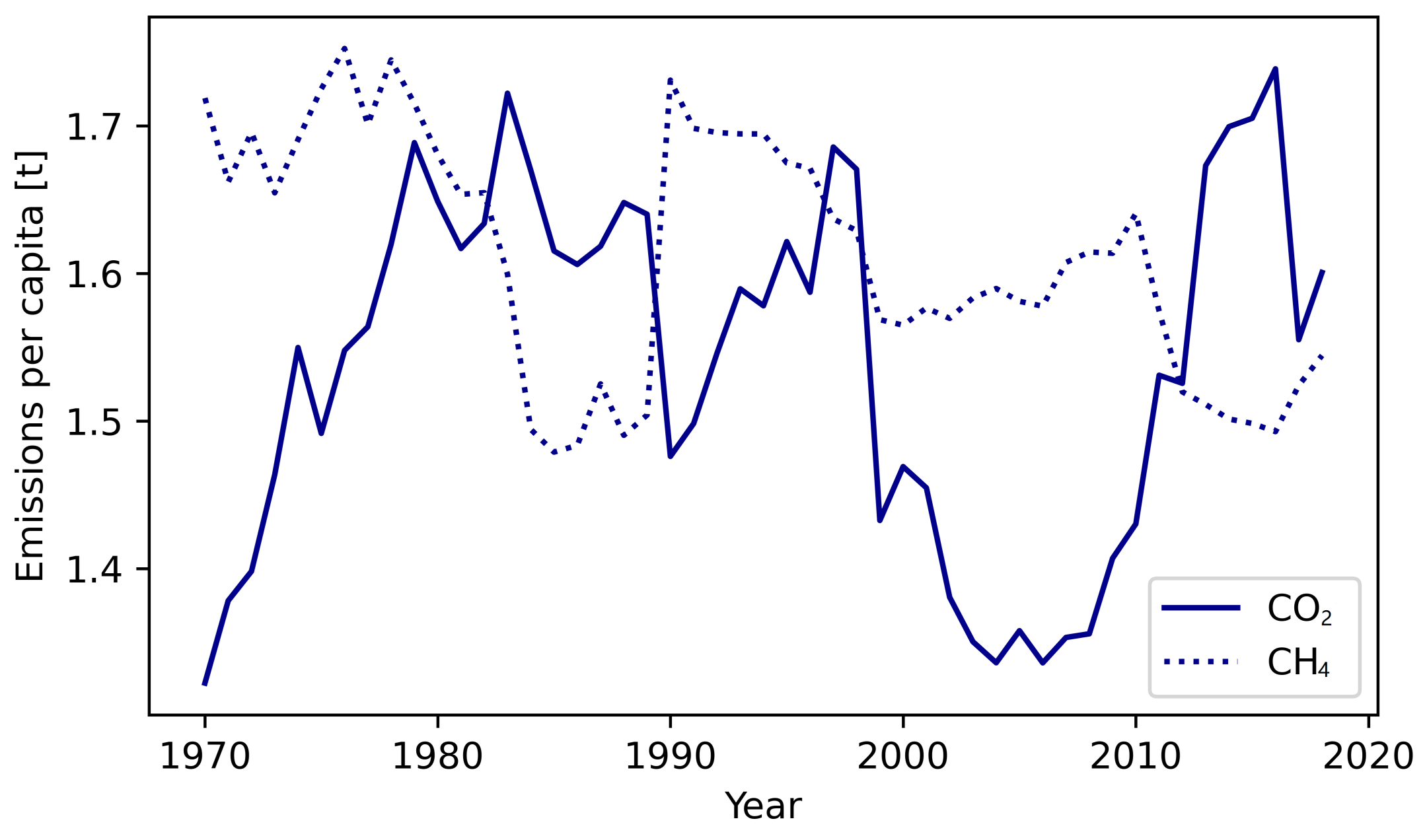
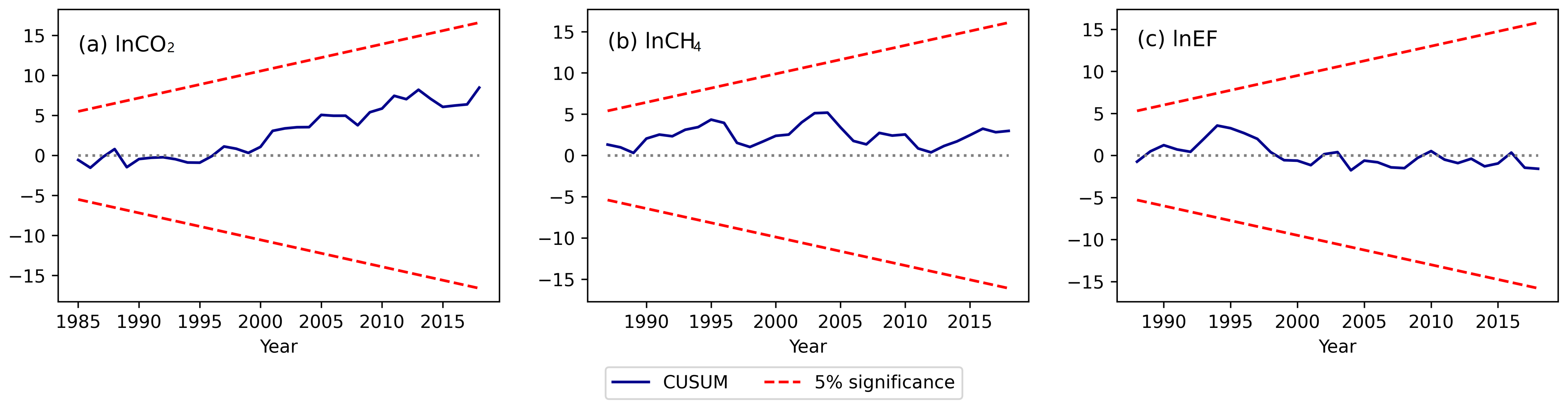
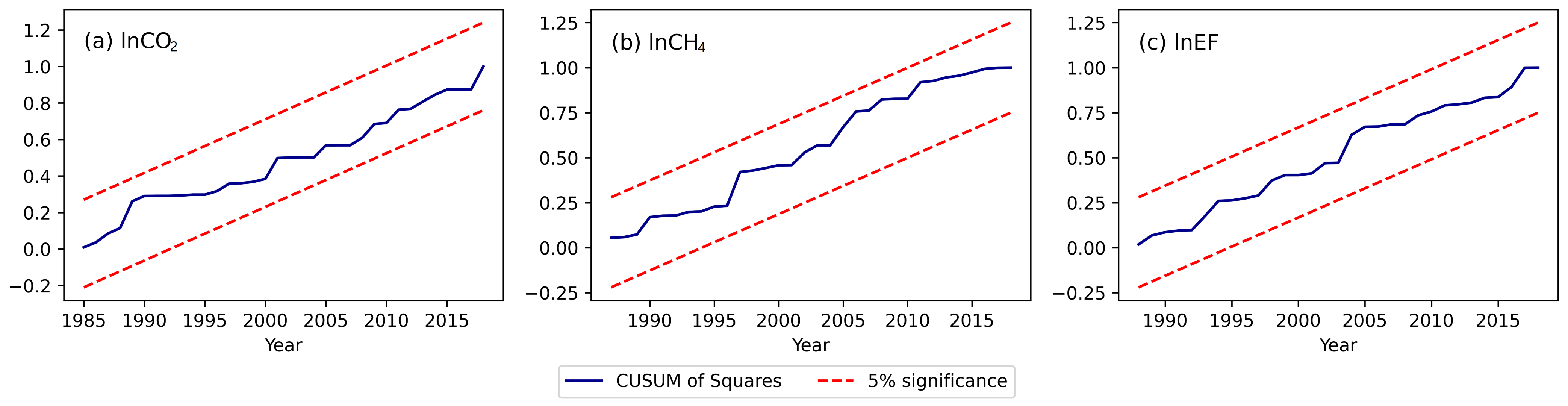
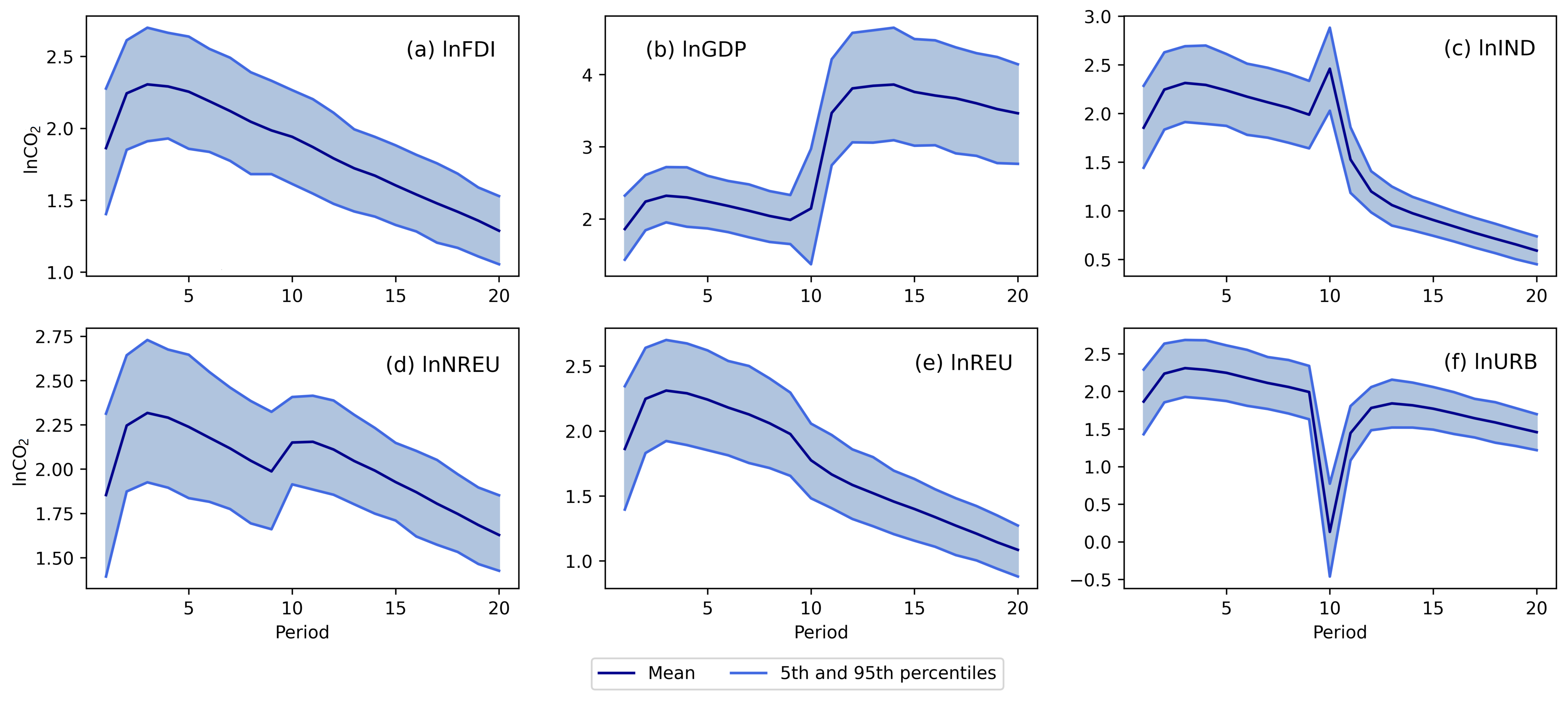
This study examined the impact of GDP per capita growth on carbon dioxide emissions, methane emissions, and the ecological footprint for a Colombian-specific case, for which there is not much research available in the literature. For this purpose, we estimated an ARDL model for each environmental degradation indicator and, in order to establish robust conclusions from it, we carried out statistical validation tests for residual normality, heteroskedasticity, serial correlation, misspecification, and structural change. After estimating each ARDL model using time series data for the period between 1970 and 2018, we found that there is a long-run robust relationship among variables, but results regarding the validity of the EKC hypothesis vary depending on the environmental degradation indicator considered. Our first model indicates that there is no evidence to validate the existence of an inverse U-shaped relationship between CO₂ emissions and GDP per capita. These results are in line with empirical findings made by [40,73] in similar studies. Despite this, our results suggest that industrialization could help to reduce CO₂ emissions in the long run, as long as it does not mean an increase in the use of energy from non-renewable sources.

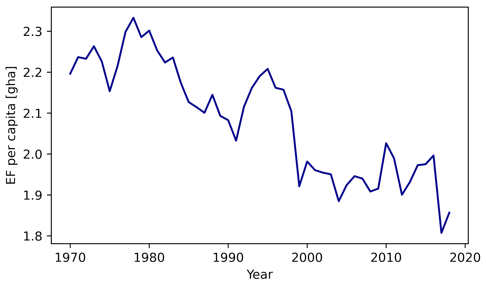
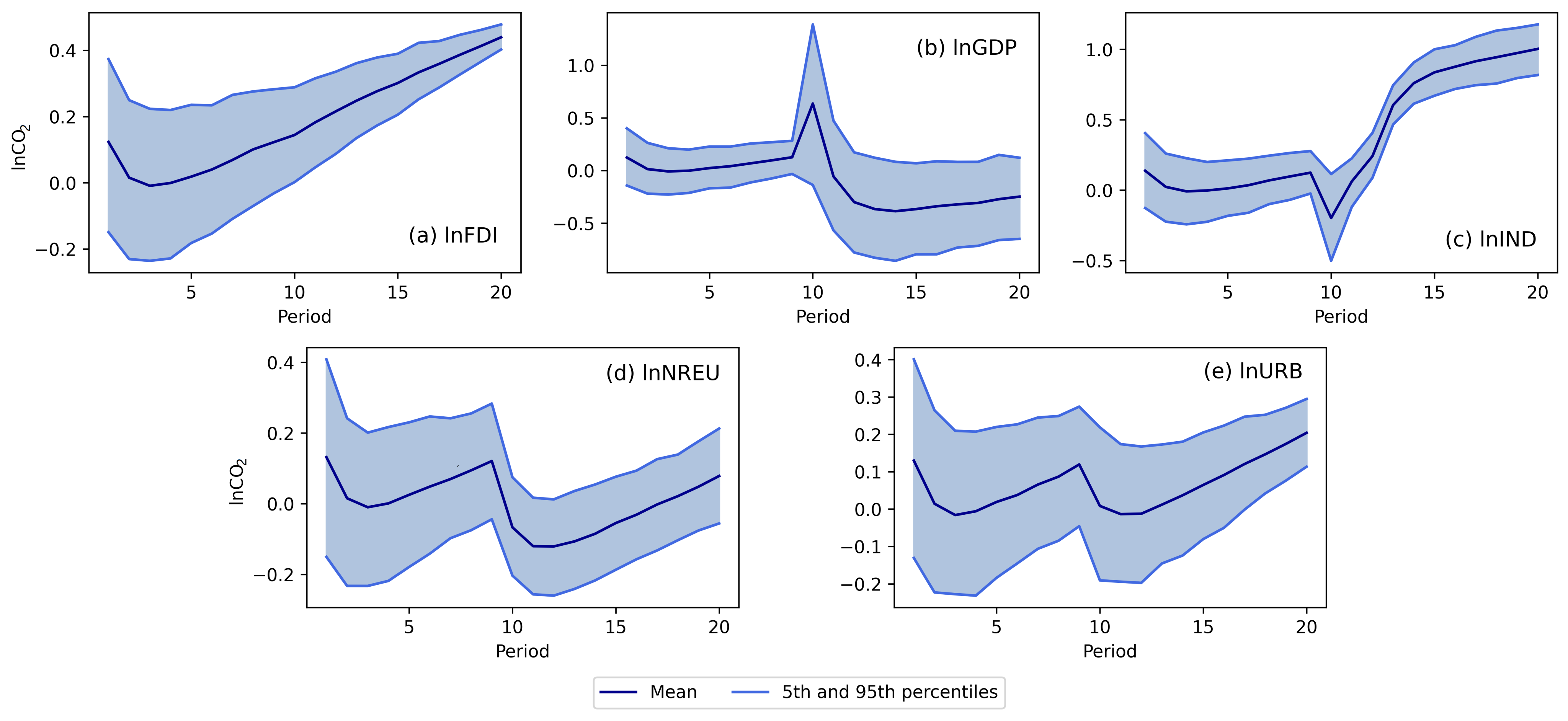
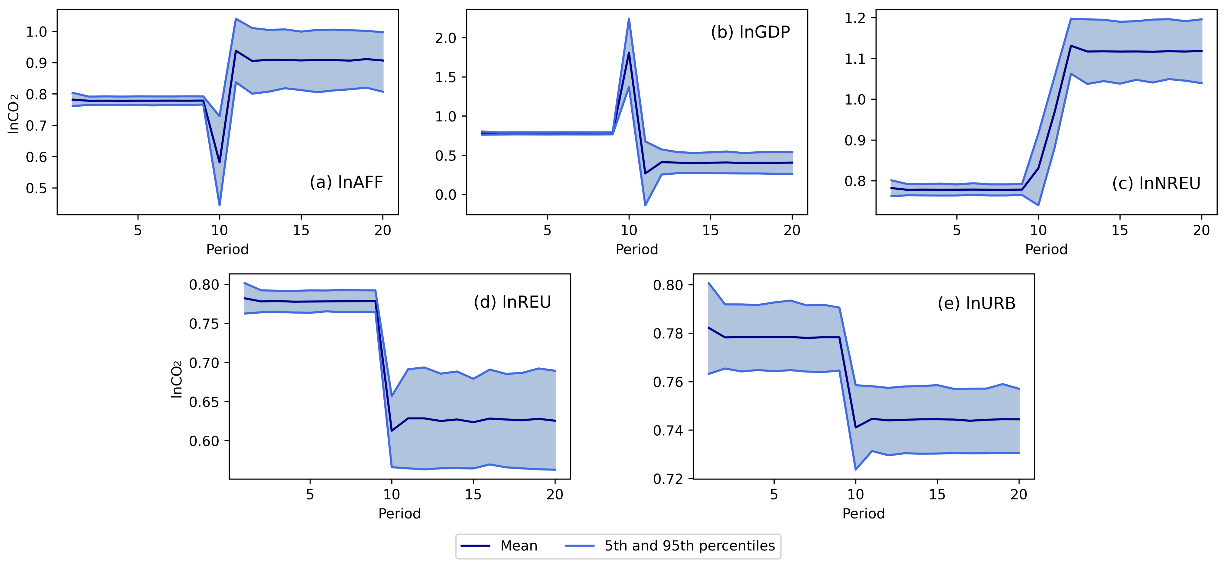
To the best of our knowledge, methane emissions and the ecological footprint have not been previously studied in the EKC framework for Colombia. We find from our models that there is statistical evidence to validate the EKC hypothesis for these environmental degradation indicators. The turning point estimated from the CH₄ model is 4113.34 constant 2015 US$ per capita, whereas the EF model indicates that the slope sign changes near to 4307.11 US$. For this last case, we find a confidence interval wider than the actual range of GDP in the sample period, but we still can conclude that economic growth can lead to an improvement in environmental quality, at least in regard to methane emissions and the ecological footprint. Moreover, the EF model results suggest that this economic growth should leverage the use of cleaner technologies and better agricultural practices as the increase in the value added of agricultural sectors will raise EF.

The effects of urbanization and foreign direct investments vary depending on the environmental indicator, and therefore it is not possible to draw general conclusions. Nevertheless, our results suggest that foreign direct investment does not have a great impact on the environment in the Colombian case as long-run elasticities are considerably low for both CO₂ and CH₄ models, and the variable is not significant for EF.

Although we cannot draw consistent conclusions as the results are mixed, the relationships studied and analyzed in this paper provide a better comprehension of the economic and environmental situation in Colombia and are relevant for climate policy design. In general, our empirical findings reinforce the necessity of shifting to renewable energy sources to achieve economic growth without harming the environment. In fact, there is evidence that economic growth could lead to reduced methane emissions and a reduced ecological footprint. For example, in Figure 7a, the dynamic simulations carried out in this study demonstrate the importance of implementing agricultural practices that involve cleaner technologies due to the contribution of this sector to GHG emissions in Colombia. Hence, investment in research, innovation, and cleaner technologies for agricultural and industrial sectors could play a key role in this process. To promote this required change from fossil fuels to cleaner energy sources, carbon taxes or incentives for companies using or investing in renewable energy could be considered. Notwithstanding, the design of these or other policies should be accompanied by broader legal, socioeconomic, and institutional assessment.

Finally, this study could be extended to include new macroeconomic variables to obtain more relevant information regarding the impact of economic development on the environment. Moreover, the econometric methodology used could be implemented to make a similar investigation focusing on regions as it may be appropriate to design region-specific policies considering differences in development, main economic activities, available natural resources, etc. However, the limited access to public and precise information is an important obstacle. Regrettably, there is not much available economic and environmental data in official Colombian sources. Instead, we used global databases, such as World Development Indicators by the World Bank [3], that can offer misleading or imprecise data for some variables. For instance, deforestation may be a relevant variable to study in Colombia as there are considerably high rates due to agriculture and cattle ranching; the creation of human settlements and roads; and illicit activities, such as illegal crops, mining, and logging, especially after the peace agreement settled in 2016 with the Revolutionary Armed Forces of Colombia (FARC) [74,75,76,77,78]. Nevertheless, information is not available annually but completed with linear interpolation, which limits the possibility to obtain useful results. Evidently, efforts should be made to improve the estimation and distribution of environmental data on public and official sources.

References

1. UNFCC. Glasgow Climate Pact | COP26. 2021. Available online: https://unfccc.int/process-and-meetings/the-paris-agreement/the-glasgow-climate-pact-key-outcomes-from-cop26 (accessed on 30 August 2022).
2. Zambrano-Monserrate, M.A.; Silva-Zambrano, C.A.; Davalos-Penafiel, J.L.; Zambrano-Monserrate, A.; Ruano, M.A. Testing environmental Kuznets curve hypothesis in Peru: The role of renewable electricity, petroleum and dry natural gas. Renew. Sustain. Energy Rev. 2018, 82, 4170–4178. [Google Scholar] [CrossRef]
3. World Bank. World Development Indicators. 2021. Available online: https://databank.worldbank.org/reports.aspx?source=world-development-indicators (accessed on 30 November 2021).
4. Price, S.F.D.; Pitts, T.R.; Van Roekel, L. Climate Change and International Responses Increasing Challenges to US National Security Through 2040: LANL Contributions to 2021 National Intelligence Estimate (No. LA-UR-21-32421); Los Alamos National Lab. (LANL): Los Alamos, NM, USA, 2021. [Google Scholar]
5. Grossman, G.M.; Krueger, A.B. Environmental Impacts of a North American Free Trade Agreement; Working Paper 3914; National Bureau of Economic Research: Cambridge, MA, USA, 1991. [Google Scholar] [CrossRef]
6. Shafik, N.; Bandyopadhyay, S. Economic Growth and Environmental Quality: Time Series and Cross-Country Evidence; Policy Research Working Paper Series 904; World Development Report; World Bank Group: Washington, DC, USA, 1992. [Google Scholar]
7. Panayotou, T. Empirical Tests and Policy Analysis of Environmental Degradation at Different Stages of Economic Development; World Employment Programme research working paper. WEP 2-22, Technology and Employment Programme; International Labour Organization: Geneva, Switzerland, 1993. [Google Scholar]
8. Sarkodie, S.A.; Strezov, V. A review on Environmental Kuznets Curve hypothesis using bibliometric and meta-analysis. Sci. Total. Environ. 2019, 649, 128–145. [Google Scholar] [CrossRef] [PubMed]
9. Charfeddine, L.; Mrabet, Z. The impact of economic development and social-political factors on ecological footprint: A panel data analysis for 15 MENA countries. Renew. Sustain. Energy Rev. 2017, 76, 138–154. [Google Scholar] [CrossRef]
10. Climate Analysis Indicators Tool (CAIT) Data Explorer. Historical Emissions. 2021. Available online: https://www.climatewatchdata.org/data-explorer/historical-emissions (accessed on 30 November 2021).
11. Van Dingenen, R.; Crippa, M.; Anssens-Maenhout, G.; Guizzardi, D.; Dentener, F. Global trends of methane emissions and their impacts on ozone concentrations. In JRC Science for Policy Report; Publications Office of the European Commission: Luxembourg, 2018. [Google Scholar]
12. Martínez-Rocamora, A.; Solís-Guzmán, J.; Marrero, M. Toward the Ecological Footprint of the use and maintenance phase of buildings: Utility consumption and cleaning tasks. Ecol. Indic. 2016, 69, 66–77. [Google Scholar] [CrossRef]
13. Al-mulali, U.; Weng-Wai, C.; Sheau-Ting, L.; Mohammed, A.H. Investigating the environmental Kuznets curve (EKC) hypothesis by utilizing the ecological footprint as an indicator of environmental degradation. Ecol. Indic. 2015, 48, 315–323. [Google Scholar] [CrossRef]
14. Wang, Y.; Kang, L.; Wu, X.; Xiao, Y. Estimating the environmental Kuznets curve for ecological footprint at the global level: A spatial econometric approach. Ecol. Indic. 2013, 34, 15–21. [Google Scholar] [CrossRef]
15. Pesaran, M.H.; Shin, Y.; Smith, R.J. Bounds testing approaches to the analysis of level relationships. J. Appl. Econom. 2001, 16, 289–326. [Google Scholar] [CrossRef]
16. Mirza, F.M.; Kanwal, A. Energy consumption, carbon emissions and economic growth in Pakistan: Dynamic causality analysis. Renew. Sustain. Energy Rev. 2017, 72, 1233–1240. [Google Scholar] [CrossRef]
17. Kuznets, S. Economic Growth and Income Inequality. Am. Econ. Rev. 1955, 45, 1–28. [Google Scholar]
18. Stern, D.I. The Environmental Kuznets Curve. In Reference Module in Earth Systems and Environmental Sciences; Elsevier: Amsterdam, The Netherlands, 2018. [Google Scholar] [CrossRef] [Green Version]
19. Beckerman, W. Economic growth and the environment: Whose growth? Whose environment? World Dev. 1992, 20, 481–496. [Google Scholar] [CrossRef]
20. Van Alstine, J.; Neumayer, E. The Environmental Kuznets Curve. In Handbook on Trade and the Environment; Gallagher, K.P., Ed.; Edward Elgar Publishing: Cheltenham, UK, 2008; Chapter 3. [Google Scholar]
21. Sarkodie, S.A.; Ozturk, I. Investigating the Environmental Kuznets Curve hypothesis in Kenya: A multivariate analysis. Renew. Sustain. Energy Rev. 2020, 117, 109481. [Google Scholar] [CrossRef]
22. Soytas, U.; Sari, R.; Ewing, B.T. Energy consumption, income, and carbon emissions in the United States. Ecol. Econ. 2007, 62, 482–489. [Google Scholar] [CrossRef]
23. Bekun, F.V.; Emir, F.; Sarkodie, S.A. Another look at the relationship between energy consumption, carbon dioxide emissions, and economic growth in South Africa. Sci. Total Environ. 2019, 655, 759–765. [Google Scholar] [CrossRef] [PubMed]
24. Fei, L.; Dong, S.; Xue, L.; Liang, Q.; Yang, W. Energy consumption-economic growth relationship and carbon dioxide emissions in China. Energy Policy 2011, 39, 568–574. [Google Scholar] [CrossRef]
25. Kivyiro, P.; Arminen, H. Carbon dioxide emissions, energy consumption, economic growth, and foreign direct investment: Causality analysis for Sub-Saharan Africa. Energy 2014, 74, 595–606. [Google Scholar] [CrossRef]
26. Sarkodie, S.A.; Strezov, V. Effect of foreign direct investments, economic development and energy consumption on greenhouse gas emissions in developing countries. Sci. Total Environ. 2019, 646, 862–871. [Google Scholar] [CrossRef]
27. Jaunky, V.C. The CO2 emissions-income nexus: Evidence from rich countries. Energy Policy 2011, 39, 1228–1240. [Google Scholar] [CrossRef]
28. Bekun, F.V.; Alola, A.A.; Sarkodie, S.A. Toward a sustainable environment: Nexus between CO2 emissions, resource rent, renewable and nonrenewable energy in 16-EU countries. Sci. Total Environ. 2019, 657, 1023–1029. [Google Scholar] [CrossRef]
29. Fodha, M.; Zaghdoud, O. Economic growth and pollutant emissions in Tunisia: An empirical analysis of the environmental Kuznets curve. Energy Policy 2010, 38, 1150–1156. [Google Scholar] [CrossRef]
30. Longo, S.; York, R. Agricultural Exports and the Environment: A Cross-National Study of Fertilizer and Pesticide Consumption. Rural. Sociol. 2008, 73, 82–104. [Google Scholar] [CrossRef]
31. Chiu, Y.B. Deforestation and the Environmental Kuznets Curve in Developing Countries: A Panel Smooth Transition Regression Approach. Can. J. Agric. Econ. Can. D’Agroecon. 2012, 60, 177–194. [Google Scholar] [CrossRef]
32. Lee, C.C.; Chiu, Y.B.; Sun, C.H. The environmental Kuznets curve hypothesis for water pollution: Do regions matter? Energy Policy 2010, 38, 12–23. [Google Scholar] [CrossRef]
33. Wong, Y.L.A.; Lewis, L. The disappearing Environmental Kuznets Curve: A study of water quality in the Lower Mekong Basin (LMB). J. Environ. Manag. 2013, 131, 415–425. [Google Scholar] [CrossRef] [PubMed]
34. Ruiz-Agudelo, C.; Sánchez, G.; Sáenz, J.; Higuera, L. Biodiversity and growth in Colombia, 1995–2015: An approach from the environmental kuznets hypothesis. J. Environ. Econ. Policy 2019, 8, 17–31. [Google Scholar] [CrossRef]
35. Al-mulali, U.; Tang, C.F.; Ozturk, I. Estimating the Environment Kuznets Curve hypothesis: Evidence from Latin America and the Caribbean countries. Renew. Sustain. Energy Rev. 2015, 50, 918–924. [Google Scholar] [CrossRef]
36. Pablo-Romero, M.; De Jesús, J. Economic growth and energy consumption: The Energy-Environmental Kuznets Curve for Latin America and the Caribbean. Renew. Sustain. Energy Rev. 2016, 60, 1343–1350. [Google Scholar] [CrossRef]
37. Vázquez, E.; García, J. Calidad ambiental y su relación con el crecimiento económico en el Área Metropolitana del Valle de Aburrá. Ecos Econ. Lat. Am. J. Appl. Econ. 2003, 7, 27–48. [Google Scholar]
38. Correa, F.; Vasco, A.; Pérez, C. La curva medioambiental de Kuznets: Evidencia empírica para Colombia Grupo de Economía Ambiental (GEA). Semestre Económico 2005, 8, 13–30. [Google Scholar]
39. Sosa, P.V.; Navarro, D.M. Crecimiento, Complejidad Económica y Emisiones de CO2: Un Análisis para Colombia. Revista CIFE: Lecturas de Economía Social 2020, 22, 21–41. [Google Scholar] [CrossRef]
40. Laverde-Rojas, H.; Guevara-Fletcher, D.A.; Camacho-Murillo, A. Economic growth, economic complexity, and carbon dioxide emissions: The case of Colombia. Heliyon 2021, 7, e07188. [Google Scholar] [CrossRef]
41. Global Footprint Network. Ecological Footprint per Person. Available online: https://data.footprintnetwork.org (accessed on 30 November 2021).
42. Ritchie, H.; Roser, M.; Rosado, P. CO2 and Greenhouse Gas Emissions. In Our World in Data; 2020; Available online: https://ourworldindata.org/co2-and-other-greenhouse-gas-emissions (accessed on 30 August 2022).
43. Ritchie, H.; Roser, M.; Rosado, P. Energy. In Our World in Data; 2020; Available online: https://ourworldindata.org/energy (accessed on 30 August 2022).
44. Poumanyvong, P.; Kaneko, S. Does urbanization lead to less energy use and lower CO2 emissions? A cross-country analysis. Ecol. Econ. 2010, 70, 434–444. [Google Scholar] [CrossRef]
45. Pesaran, H.; Shin, Y. An Autoregressive Distributed-Lag Modelling Approach to Cointegration Analysis. In Econometrics and Economic Theory in the 20th Century: The Ragnar Frisch Centennial Symposium; Cambridge University Press: Cambridge, UK, 1995; pp. 371–413. [Google Scholar] [CrossRef]
46. Philips, A.Q. Have Your Cake and Eat It Too? Cointegration and Dynamic Inference from Autoregressive Distributed Lag Models. Am. J. Political Sci. 2018, 62, 230–244. [Google Scholar] [CrossRef] [Green Version]
47. Pfaff, B. Analysis of Integrated and Cointegrated Time Series with R; Springer Science+Business Media, LLC: New York, NY, USA, 2006. [Google Scholar]
48. Jarque, C.M.; Bera, A.K. Efficient tests for normality, homoscedasticity and serial independence of regression residuals. Econ. Lett. 1980, 6, 255–259. [Google Scholar] [CrossRef]
49. Breusch, T.S.; Pagan, A.R. A simple test for heteroscedasticity and random coefficient variation. Econom. J. Econom. Soc. 1979, 47, 1287–1294. [Google Scholar] [CrossRef]
50. Breusch, T.S. Testing for autocorrelation in dynamic linear models. Aust. Econ. Pap. 1978, 17, 334–355. [Google Scholar] [CrossRef]
51. Ramsey, J.B. Tests for specification errors in classical linear least-squares regression analysis. J. R. Stat. Soc. Ser. B Methodol. 1969, 31, 350–371. [Google Scholar] [CrossRef]
52. Brown, R.L.; Durbin, J.; Evans, J.M. Techniques for testing the constancy of regression relationships over time. J. R. Stat. Soc. Ser. B Methodol. 1975, 37, 149–163. [Google Scholar] [CrossRef]
53. Pesaran, M.; Pesaran, B. Working with Microfit 4.0: Interactive Econometric Analysis; Oxford University Press: Oxford, UK, 1997. [Google Scholar]
54. Jordan, S.; Philips, A.Q. Dynamic Simulation and Testing for Single-Equation Cointegrating and Stationary Autoregressive Distributed Lag Models. R J. 2018, 10, 469–488. [Google Scholar] [CrossRef] [Green Version]
55. Narayan, P.K. The saving and investment nexus for China: Evidence from cointegration tests. Appl. Econ. 2005, 37, 1979–1990. [Google Scholar] [CrossRef]
56. Williams, L.; Whitten, G. Dynamic Simulations of Autoregressive Relationships. Stata J. 2011, 11, 577–588. [Google Scholar] [CrossRef]
57. Lind, J.T.; Mehlum, H. With or Without U? The Appropriate Test for a U-Shaped Relationship. Oxf. Bull. Econ. Stat. 2010, 72, 109–118. [Google Scholar] [CrossRef] [Green Version]
58. Fieller, E.C. Some Problems in Interval Estimation. J. R. Stat. Soc. Ser. B Methodol. 1954, 16, 175–185. [Google Scholar] [CrossRef]
59. Schwert, G.W. Tests for Unit Roots: A Monte Carlo Investigation. J. Bus. Econ. Stat. 1989, 7, 147–159. [Google Scholar]
60. Ahmad, A.; Zhao, Y.; Shahbaz, M.; Bano, S.; Zhang, Z.; Wang, S.; Liu, Y. Carbon emissions, energy consumption and economic growth: An aggregate and disaggregate analysis of the Indian economy. Energy Policy 2016, 96, 131–143. [Google Scholar] [CrossRef]
61. Heidari, H.; Katircioğlu, S.T.; Saeidpour, L. Economic growth, CO2 emissions, and energy consumption in the five ASEAN countries. Int. J. Electr. Power Energy Syst. 2015, 64, 785–791. [Google Scholar] [CrossRef]
62. Hu, H.; Xie, N.; Fang, D.; Zhang, X. The role of renewable energy consumption and commercial services trade in carbon dioxide reduction: Evidence from 25 developing countries. Appl. Energy 2018, 211, 1229–1244. [Google Scholar] [CrossRef]
63. Saidi, K.; Mbarek, M.B. The impact of income, trade, urbanization, and financial development on CO2 emissions in 19 emerging economies. Environ. Sci. Pollut. Res. 2017, 24, 12748–12757. [Google Scholar] [CrossRef]
64. Antonakakis, N.; Chatziantoniou, I.; Filis, G. Energy consumption, CO2 emissions, and economic growth: An ethical dilemma. Renew. Sustain. Energy Rev. 2017, 68, 808–824. [Google Scholar] [CrossRef] [Green Version]
65. Wang, S.; Li, Q.; Fang, C.; Zhou, C. The relationship between economic growth, energy consumption, and CO2 emissions: Empirical evidence from China. Sci. Total Environ. 2016, 542, 360–371. [Google Scholar] [CrossRef]
66. Djoukouo, A.F.D. Relationship between methane emissions and economic growth in Central Africa countries: Evidence from panel data. Glob. Transitions 2021, 3, 126–134. [Google Scholar] [CrossRef]
67. Saunois, M.; Stavert, A.R.; Poulter, B.; Bousquet, P.; Canadell, J.G.; Jackson, R.B.; Raymond, P.A.; Dlugokencky, E.J.; Houweling, S.; Patra, P.K.; et al. The Global Methane Budget 2000–2017. Earth Syst. Sci. Data 2020, 12, 1561–1623. [Google Scholar] [CrossRef]
68. United Nations Environment Programme. Global Methane Assessment: Benefits and Costs of Mitigating Methane Emissions; 2021; Available online: https://www.unep.org/resources/report/global-methane-assessment-benefits-and-costs-mitigating-methane-emissions (accessed on 30 August 2022).
69. Narayan, P.K.; Smyth, R. What determines migration flows from low-income to high-income countries? An empirical investigation of Fiji-U.S. migration 1972–2001. Contemp. Econ. Policy 2006, 24, 332–342. [Google Scholar] [CrossRef]
70. Destek, M.A.; Sarkodie, S.A. Investigation of environmental Kuznets curve for ecological footprint: The role of energy and financial development. Sci. Total Environment 2019, 650, 2483–2489. [Google Scholar] [CrossRef] [PubMed]
71. Calderón, S.; Alvarez, A.C.; Loboguerrero, A.M.; Arango, S.; Calvin, K.; Kober, T.; Daenzer, K.; Fisher-Vanden, K. Achieving CO2 reductions in Colombia: Effects of carbon taxes and abatement targets. Energy Econ. 2016, 56, 575–586. [Google Scholar] [CrossRef] [Green Version]
72. Bugge, M.M.; Hansen, T.; Klitkou, A. What Is the Bioeconomy? A Review of the Literature. Sustainability 2016, 8, 691. [Google Scholar] [CrossRef] [Green Version]
73. Blanco Camargo, M.; Hernández Orozco, S.; Fajardo Ortiz, E.; Romero-Valbuena, H. Consumption of energy, economic growth, and carbon dioxide emissions in Colombia. Revista Fuentes: El Reventón Energético 2020, 18, 41–501. [Google Scholar] [CrossRef]
74. Etter, A.; McAlpine, C.; Possingham, H. Historical Patterns and Drivers of Landscape Change in Colombia Since 1500: A Regionalized Spatial Approach. Ann. Assoc. Am. Geogr. 2008, 98, 2–23. [Google Scholar] [CrossRef]
75. Armenteras, D.; Cabrera, E.; Rodríguez, N.; Retana, J. National and regional determinants of tropical deforestation in Colombia. Reg. Environ. Chang. 2013, 13, 1181–1193. [Google Scholar] [CrossRef]
76. Chadid, M.A.; Dávalos, L.M.; Molina, J.; Armenteras, D. A Bayesian Spatial Model Highlights Distinct Dynamics in Deforestation from Coca and Pastures in an Andean Biodiversity Hotspot. Forests 2015, 6, 3828–3846. [Google Scholar] [CrossRef] [Green Version]
77. Liévano-Latorre, L.F.; Brum, F.T.; Loyola, R. How effective have been guerrilla occupation and protected areas in avoiding deforestation in Colombia? Biol. Conserv. 2021, 253, 108916. [Google Scholar] [CrossRef]
78. Clerici, N.; Armenteras, D.; Kareiva, P.; Botero, R.; Ramírez-Delgado, J.; Forero-Medina, G.; Ochoa, J.; Pedraza, C.; Schneider, L.; Lora, C.; et al. Deforestation in Colombian protected areas increased during post-conflict periods. Sci. Rep. 2020, 10, 4971. [Google Scholar] [CrossRef] [PubMed] [Green Version]
Figure 1. Annual CO2 and CH4 emissions per capita.
Sustainability 15 03738 g001
Figure 2. Annual ecological footprint per capita.
Sustainability 15 03738 g002
Figure 3. Cumulative sum control chart for (a) lnCO2 model, (b) lnCH4 model, and (c) lnEF model.
Sustainability 15 03738 g003
Figure 4. Cumulative sum of squares control chart for (a) lnCO2 model, (b) lnCH4 model, and (c) lnEF model.
Sustainability 15 03738 g004
Figure 5. The effect on CO2 emissions of a 10% increase in (a) lnFDI, (b) lnGDP, (c) lnIND, (d) lnNREU, (e) lnREU, and (f) lnURB in period 10, while holding the remaining variables at their means.
Sustainability 15 03738 g005
Figure 6. The effect on CH4 emissions of a 10% increase in (a) lnFDI, (b) lnGDP, (c) lnIND, (d) lnNREU, and (e) lnURB in period 10, while holding the remaining variables at their means.
Sustainability 15 03738 g006
Figure 7. The effect on ecological footprint of a 10% increase in (a) lnAFF, (b) lnGDP, (c) lnNREU, (d) lnREU, and (e) lnURB in period 10, while holding the remaining variables at their means.
Sustainability 15 03738 g007