Decision-Making of Cross-Border E-Commerce Platform Supply Chains Considering Information Sharing and Free Shipping

Abstract

For cross-border e-commerce companies with high shipping costs, the existing retailer and the new entrant retailer on the platform are usually concerned with information sharing and free shipping due to the uncertainty of market demand. For this, by establishing a Stackelberg game model between two competing retailers, we analyze the strategy of retailers and explore the business strategies of the cross-border e-commerce platform. The study shows that regarding information-sharing strategies, retailer A’s willingness to share information is positively related to initial market potential and negatively related to market competition intensity. Moreover, retailer B is willing to spend higher information costs to purchase information when the necessity of the product is more elevated. As for a free shipping strategy, if the existing retailer offers free shipping, the new entrant retailer should also offer free shipping service to consumers when the initial market potential is larger. Conversely, when the initial market potential is smaller, the retailer’s willingness to offer free shipping decreases when the intensity of competition in the market increases. When the market tends to be perfectly competitive, the new entrant retailer will not choose a free shipping strategy, and the platform is most profitable when information sharing and free shipping occur simultaneously. However, when the carrier charges a higher shipping fee to customers, the existing retailer is more profitable when the new entrant does not offer free shipping. Therefore, in order to achieve a win-win situation for all parties, the platform needs to develop appropriate operational strategies to influence the decisions of retailers and carriers. Some numerical experiments are made to test the validity of the model and the effect of the parameters involved in the model.

1. Introduction

E-commerce has become a top priority for many businesses around the world [1]. Developing e-commerce can increase sales and profits and offer the opportunity to overcome obstacles to growth [2]. With the development of internet technology, e-commerce has enabled cross-border transactions and become the fastest-growing industry in the global economy [3]. Global cross-border e-commerce (CBEC) was worth over $\$780$ billion in 2019 [4]. The e-commerce business rapidly grew due to COVID-19. Even the most basic survival products, such as food, turned to the Internet because e-commerce was considered more convenient than offline [5]. Significantly affected by COVID-19, Amazon’s net sales in 2020 were $\$386.06$ billion, an increase of $37.6\%$ from $\$280.52$ billion in 2019. Meanwhile, data from the General Administration of Customs show that in 2021, the scale of China’s cross-border e-commerce exports reached $1.98$ trillion yuan, up $15\%$ year-on-year. The boom in CBEC has dramatically enriched the trading market in various countries. However, ICT, the political and regulatory environment, and human resource influence the development of global e-commerce [6], therefore, supply chain shortages and many other global supply chain issues in the post-epidemic era suggest that cross-border e-commerce will slow down in the near future. How to effectively control and manage the platform logistics and supply chain is a critical issue for an e-commerce platform.

To better serve overseas customers, many retailers offer free shipping services. For example, Xiaomi, a famous Chinese smartphone brand, offers free shipping through the cross-border e-commerce platform AliExpress. Temu, the cross-border e-commerce export platform of Pinduoduo, launches with the slogan “free shipping” prominently. Note that shipping and handling costs are causing $52\%$ of people to abandon online shopping. Thus, free shipping has a more significant impact on buyers than price discounts [7]. Shehu et al. [8] believe that free shipping promotions encourage customers to buy riskier items. Thus, offering free shipping services may be an important marketing decision [9].

E-commerce retailers selling products through the platform will accumulate a large amount of data information on the platform. With the growth of e-commerce, information sharing has a great influence on online sales [10]. In the face of uncertain market demand, retailers can process past sales data through machine learning such as the Apriori-based clustering algorithm [11] and the improved genetic algorithm [12] to make more accurate predictions. For cross-border companies with long distances and high costs, information sharing is likely to influence their free shipping and quantitative decisions. Empirical evidence suggests that only $27\%$ of retailers share POS (Point of Sale) data with other members [13]. How to facilitate information sharing among retailers on the platform is an essential issue for the platform to consider.

For competition in the CBEC platform, Lv [14] studies the revenue management of the CBEC platform and the competition and coordination between platform suppliers and e-retailers through supply chain decision-making. Lu et al. [15] explore consumers’ willingness to select CBEC platforms and the factors effecting them. Zha et al. [16] research the information sharing strategies of CBEC platforms and the choices of overseas suppliers regarding direct-mail logistics mode and bonded warehouse logistics mode. Qi et al. [17] and Cao et al. [18] study the willingness of traditional retailers to enter e-commerce platforms, and the willingness of retailers and platforms to share their private information if they do. Jiang et al. [19] study the Amazon platform’s choice of sales model in the face of uncertain market demand.

For free shipping in e-commerce, Li et al. [20] research free shipping policies for e-commerce under the add-on item recommendation service. Wang and Li [21] study supply chain decisions in e-commerce considering the cost of logistics services and the “free shipping” strategy. Han et al. [22] study the free shipping policy of CBEC based on consumer decision theory. Hua et al. [7] study the optimal order quantity and optimal retail price for retailers, assuming that suppliers offer free shipping, and find that free shipping can benefit suppliers, retailers, and end customers. Etumnu [23] studies the impact of free shipping on grocery sales on Amazon’s CBEC platform and found that products with free shipping garnered more sales. Leng and Becerril-Arreola [24] examine the effect of e-commerce retailers’ free shipping strategies on consumer purchase behavior. Rui et al. [25] analyze the impact of the free shipping strategy on supply chain members based on the Stackelberg game, and provide theoretical support for e-retailers and consumers to make optimal decisions. Niu et al. [9] examine the free shipping decisions of two competing retailers in CBEC when relying on the same carrier to transport goods.

As for information sharing, the previous literature primarily focuses on the motivations for vertical information sharing upstream and downstream of the supply chain [26,27,28,29,30,31]. A few studies address horizontal information sharing motives between competitors. Kirby [32] examines the incentives of firms competing in an oligopolistic industry to share information about an unknown demand when such sharing takes place on the basis of exchange. Niu et al. [33] examine whether incumbent carriers with demand information have an incentive to disclose demand information to new carriers in cross-border logistics. Liu et al. [34] study strategies for retail platforms to share demand information to sellers on the platform. Mukhopadhyay et al. [35] study the information sharing strategies of two independent companies with market demand information under the Stackelberg game and devise a “simple to implement” information sharing scheme under which both firms and the total system are better off. To summarize, the relevant studies are shown in

Table 1. Contribution of this paper and related literature.

	E-Commerce	E-Commerce Platform	Free Shipping	Information Sharing	Competition
Li and Zhang [26]	√			√	√
Mukhopadhyay et al. [35]	√			√	√
Liu et al. [34]	√			√	√
Wang and Li [21]	√		√		√
Rui et al. [25]	√		√		√
Niu et al. [9]	√		√		√
Cao et al. [18]	√	√		√	√
Zha et al. [16]	√	√		√	√
Our paper	√	√	√	√	√

. Our paper integrates the competition among retailers considering information sharing and free shipping on CBEC platforms, and analyzes the business decision-making of the e-commerce platform.

For cross-border e-commerce companies with high shipping costs, due to market demand uncertainty, retailers on the platform usually care about information sharing and free shipping. Based on the above analysis, we study the competition between an existing retailer and a new retailer on the CBEC platform under information asymmetry. The retailer needs to decide whether to share information and whether to provide free shipping. We assume the CBEC platform operates using a marketplace model similar to a revenue-sharing scheme, where the platform receives a commission from each online sale [36]. For this model, we consider the following issues:

(1)

Considering the impact of free shipping on consumers’ willingness to buy, under what circumstances would retailers choose to offer free shipping services?

(2)

Is the retailer with information willing to share it? Is the new entrant willing to obtain information? Is the platform willing to enable information sharing?

(3)

Which is an equilibrium strategy for competing retailers’ decisions on information sharing, free shipping, and quantity?

(4)

How should the CBEC platform develop business strategies to achieve a win–win–win situation in the marketplace mode?

Business strategies represent drivers and constraints of strategic choice [37]. This study constructs four Stackelberg game supply chain models to address these issues, such as the research approach adopted by Qu et al. [38]. We derive analytical expressions for optimal decision-making and profit in different scenarios [39], investigate the strategies of existing and new entrant retailers in terms of information sharing and free shipping, and further analyze the platform’s business strategy.

The remainder of this paper is organized as follows. Section 2 describes the model. Section 3 analyzes the decision preferences of retailers by comparing the equilibrium results under the four scenarios. Section 4 presents the numerical studies. The derivation procedure of the equilibrium results, the proof of propositions, and the equilibrium results of the extended model are listed in the Appendix A.

2. Model Description and Notations

In the information problem, Niu et al. [40] and Xing et al. [41] describe information asymmetry with mean and variance, where the lower (higher) information variance implies more (less) accurate demand forecasts. In the problem of free shipping, Niu et al. [9] construct a game model between two competing retailers from the perspective of consumers’ utility and profit functions of supply chain parties to solve the problem of free shipping in cross-border e-commerce. Therefore, our paper considers the maximization of profit for each party in the supply chain, constructs the game model using the inverse demand function derived from the consumer utility function, and describes the information asymmetry by mean and variance. Suppose the e-commerce platform with a retailer (denoted A) and a new entrant retailer (denoted B), the two retailers sell the same product to overseas customers on the same CBEC platform (denoted P) with the marketplace mode, and they ship their products through a common carrier (denoted C). See Figure 1 for the running pattern of the model.

Assume retailer A has been operating on the platform for a long time and has a large amount of sales data, and he can more accurately predict market demand. Retailer B is a newcomer without much information on the market’s demand. The platform will create opportunities for information sharing between existing retailers and new entrant retailers to maintain the diversity of the system. If retailer A chooses to share information, retailer B may purchase this information from the platform, and can also decline to buy the information. Certainly, to encourage the existing retailer to share information, the platform will make compensation if the new entrant retailer chooses to purchase sales information. For simplicity, we set the information purchase fee and the amount of compensation to be equal and denote it with F.

Now, we examine the strategic choices of existing retailer A and new entrant retailer B in terms of both information and shipping fees. As for the information interchange, we consider two scenarios: (1) Retailer B obtains information (labeled Scenario Y); (2) Retailer B does not obtain information (labeled Scenario N). As for free shipping, when customers buy products from retailer A, he offers free shipping service. That is, customers need only pay for the products, and the shipping fee is paid by retailer A. For retailer B, she has two options: (1) offering free shipping service like retailer A, denoting this choice as Strategy II; (2) Selling products without free shipping, and the customers need to pay for both product and the shipping service separately. We denote this choice as strategy IN. Combining the information sharing and free shipping strategies, either Strategy II or Strategy IN may occur under both Scenario Y and Scenario N. We further subdivide Scenarios Y and N into four scenarios (Y_II, Y_IN, N_II, N_IN) to describe all possible outcomes.

To proceed, we summarize the notations and descriptions in

Table 2. Notations and explanations.

Parameters	Meaning
a	Initial market potential
$\epsilon$	Demand uncertainty
$\beta$	Price sensitivity to its own quantity
$\gamma$	Price sensitivity to its rivals’ quantity
$\eta$	Platform’s commission rate with marketplace mode
F	Information purchase fee
${\pi }_i$	The profit of i, where $i=A,B,P$
$q_i$	Sales quantity of retailers, where $i=A,B$
$p_i$	Unit product price, where $i=A,B$
${\omega }_0$	Unit shipping fee charged to retailers by the carrier
${\omega }_1$	Unit shipping fee charged to overseas customers by the carrier

in which subscripts A, B, C, and P are added to refer to solutions for the existing retailer, new entrant retailer, carrier, and platform.

2.1. Demand Function

From the analysis above, we can obtain the following quadratic utility function [42]:

$$U\left(q_{A,}{q}_B\right)=A_A{q}_A+A_B{q}_B-\frac{1}{2}\left(a_A{q}_A^2+2b{q}_A{q}_B+a_B{q}_B^2\right)$$

(1)

where $A_i(i=A,B)$ denotes the market potential of product i during a period, $q_i$ is the sales amount of product i in the same period, $a_i$ denotes the effect of the quantity of product i on consumers’ utility, and parameter b captures the interactions among the products which denotes the measure of product substitutability or complementarity. The consumer utility decreases as products become more substitutable (i.e., when $b>0$, $U\left(q_{A,}{q}_B\right)$ decreases as b increases). To ensure strict concavity of the utility function and the demand quantities to be positive, we set $A_i>0$, $a_i>0$, $a_j{A}_i-b{A}_j>0$, for $i,j=A,B$ and $i\ne j$, $a_A{a}_B-b^2>0$. Assume that products A and B are substitutable, $U\left(q_A,q_B\right)$ is symmetric in products A and B. Then we can let $A_A=A_B=a$, $a_A=a_B=\beta$, and the product substitutability $b=r(r>0)$. As consumers only pay $p_A$ or $p_B$ for the buying product when the retailer offers free shipping, the consumer surplus $R(q_A,q_B)$ under different free shipping strategies can be expressed as consumer utility minus the cost paid [9]:

Strategy II:

$$R\left(q_{A,}{q}_B\right)=a{q}_A+a{q}_B-\frac{1}{2}\left(\beta q_A^2+2\gamma q_A{q}_B+\beta q_B^2\right)-p_A{q}_A-p_B{q}_B$$

(2)

Strategy IN:

$$R\left(q_{A,}{q}_B\right)=a{q}_A+a{q}_B-\frac{1}{2}\left(\beta q_A^2+2\gamma q_A{q}_B+\beta q_B^2\right)-p_A{q}_A-\left(p_B+{\omega }_1\right)q_B$$

(3)

where $a>0,\beta >\left|\gamma \right|\ge 0$. As the demand is uncertain, inverse demand functions can be obtained by maximizing the consumer surplus function

Strategy II:

$$p_A^{\mathrm{i}\_\mathrm{II}}=a+\epsilon -\beta q_A-\gamma q_B$$

(4)

$$p_B^{\mathrm{i}\_\mathrm{II}}=a+\epsilon -\beta q_B-\gamma q_A$$

(5)

Strategy IN:

$$p_A^{\mathrm{i}\_\mathrm{IN}}=a+\epsilon -\beta q_A-\gamma q_B$$

(6)

$$p_B^{\mathrm{i}\_\mathrm{IN}}=a+\epsilon -\beta q_B-\gamma q_A-{\omega }_1$$

(7)

for $i\in \{Y,N\}$.

Here, a is the initial market potential, and coefficients $\beta$ and $\gamma$ indicate the sensitivity of price to the retailer’s own and rival quantities, respectively. We assume that $1\ge \beta >\gamma >0$ and denote $\gamma$ the intensity of competition (a larger $\gamma$ indicates a more competitive market).

We use the random variable $\epsilon$ to describe the market demand that obeys the normal distribution with $E\left[\epsilon \right]=0$ and $Var\left[\epsilon \right]={\sigma }^2$. Retailer A has the data information, so its demand forecast is $\mathrm{\Gamma }=\epsilon +{\epsilon }_1$. If retailer A shares information with retailer B, retailer B’s demand forecast is also $\mathrm{\Gamma }=\epsilon +{\epsilon }_1$, where ${\epsilon }_1$ an independent random variable that follows the normal distribution with ${\epsilon }_1\sim N\left(0,{\sigma }_1^2\right)$, ${\sigma }^2>{\sigma }_1^2$, and $\frac{{\sigma }^2}{{\sigma }^2+{\sigma }_1^2}\in \left(\frac{1}{2},1\right)$. According to the discussion by Roy [43] and Niu et al. [40], we can obtain

$$E\left[\epsilon \left|\mathrm{\Gamma }\right.\right]=\frac{{\sigma }^2\mathrm{\Gamma }}{{\sigma }^2+{\sigma }_1^2}=\frac{{\sigma }^2\left(\epsilon +{\epsilon }_1\right)}{{\sigma }^2+{\sigma }_1^2},$$

(8)

$$V\left[\epsilon \left|\mathrm{\Gamma }\right.\right]=\frac{{\sigma }^2{\sigma }_1^2}{{\sigma }^2+{\sigma }_1^2}.$$

(9)

Certainly, when the demand signal is obtained, the variance of the demand forecast becomes smaller, namely, $V\left[\epsilon \left|\mathrm{\Gamma }\right.\right]<{\sigma }^2$, and the accuracy of the forecast increases.

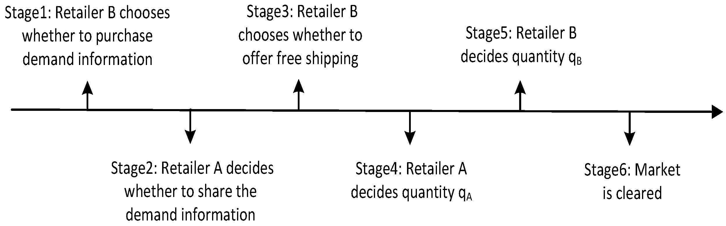
2.2. Events and Profit Functions

According to Figure 1, we can construct a Stackelberg game to study the supply chain decision as shown in Figure 2 for the sequence of game occurrence. In the first stage, new entrant retailer B chooses whether to purchase demand information from the platform. In the second stage, if retailer B chooses to buy the information, retailer A should decide whether to share the demand information or not. In the third stage, retailer B chooses whether to offer free shipping services. In the fourth stage, retailer A decides the optimal order quantity, and in the fifth stage, retailer B determines the optimal order quantity. Finally, when demand is realized, the market is cleared.

With uncertain market demand, the expected profits of retailer A, retailer B, and platform P under different scenarios depend on the demand forecast. Suppose that carrier C transports goods from multiple manufacturers, and its profit is independent of the market demand forecast. We maximize the profits of retailers A and B, respectively, and solve this game using backward induction. The equilibrium results of each situation are summarized in

Table A1. Equilibrium results under different scenarios.

Y_II	$q_A^{\mathrm{Y}\_\mathrm{II}}=\frac{\left(a-{\omega }_0\right)(2\beta -\gamma )}{4{\beta }^2-2{\gamma }^2}+\frac{(2\beta -\gamma )E\left[\epsilon \right|\mathrm{\Gamma }]}{4{\beta }^2-2{\gamma }^2}$
	$q_B^{\mathrm{Y}\_\mathrm{II}}=\frac{\left(a-{\omega }_0\right)\left(4{\beta }^2-2\beta \gamma -{\gamma }^2\right)}{8{\beta }^3-4\beta {\gamma }^2}+\frac{\left(4{\beta }^2-2\beta \gamma -{\gamma }^2\right)E\left[\epsilon \right|\mathrm{\Gamma }]}{8{\beta }^3-4\beta {\gamma }^2}$
	$p_A^{\mathrm{Y}\_\mathrm{II}}=\frac{a(2\beta -\gamma )+{\omega }_0(2\beta +\gamma )}{4\beta }+\frac{(2\beta -\gamma )E\left[\epsilon \right|\mathrm{\Gamma }]}{4\beta }$
	$p_B^{\mathrm{Y}\_\mathrm{II}}=\frac{a\left(4{\beta }^2-2\beta \gamma -{\gamma }^2\right)+{\omega }_0\left(4{\beta }^2+2\beta \gamma -3{\gamma }^2\right)}{8{\beta }^2-4{\gamma }^2}+\frac{\left(4{\beta }^2-2\beta \gamma -{\gamma }^2\right)E\left[\epsilon \right|\mathrm{\Gamma }]}{8{\beta }^2-4{\gamma }^2}$
	$E\left[\left.{\pi }_A^{\mathrm{Y}\_\mathrm{II}}\right|\mathrm{\Gamma }\right]=F+\frac{(1-\eta ){(\gamma -2\beta )}^2\left(a-{\omega }_0\right){}^2}{16{\beta }^3-8\beta {\gamma }^2}+\frac{(1-\eta ){(\gamma -2\beta )}^2}{16{\beta }^3-8\beta {\gamma }^2}\times \frac{{\sigma }^4}{{\sigma }^2+{\sigma }_1^2}$
	$E\left[\left.{\pi }_B^{\mathrm{Y}\_\mathrm{II}}\right|\mathrm{\Gamma }\right]=-F+\frac{(1-\eta ){\left(-4{\beta }^2+2\beta \gamma +{\gamma }^2\right)}^2\left(a-{\omega }_0\right){}^2}{16\beta {\left({\gamma }^2-2{\beta }^2\right)}^2}+\frac{(1-\eta ){\left(-4{\beta }^2+2\beta \gamma +{\gamma }^2\right)}^2}{16\beta {\left({\gamma }^2-2{\beta }^2\right)}^2}\times \frac{{\sigma }^4}{{\sigma }^2+{\sigma }_1^2}$
	$E\left[{\pi }_P^{\mathrm{Y}\_\mathrm{II}}\right]=\frac{\eta \left(a^2-2a{\omega }_0+{\omega }_0^2\right)\left(32{\beta }^4-32{\beta }^3\gamma -8{\beta }^2{\gamma }^2+12\beta {\gamma }^3-{\gamma }^4\right)}{16\beta {\left({\gamma }^2-2{\beta }^2\right)}^2}+\frac{\eta \left(32{\beta }^4-32{\beta }^3\gamma -8{\beta }^2{\gamma }^2+12\beta {\gamma }^3-{\gamma }^4\right)}{16\beta {\left({\gamma }^2-2{\beta }^2\right)}^2}\times \frac{{\sigma }^4}{{\sigma }^2+{\sigma }_1^2}$
Y_IN	$q_A^{\mathrm{Y}\_\mathrm{IN}}=\frac{a(2\beta -\gamma )-2\beta {\omega }_0+\gamma {\omega }_1}{4{\beta }^2-2{\gamma }^2}+\frac{(2\beta -\gamma )E\left[\epsilon \right|\mathrm{\Gamma }]}{4{\beta }^2-2{\gamma }^2}$
	$q_B^{\mathrm{Y}\_\mathrm{IN}}=\frac{a\left(4{\beta }^2-2\beta \gamma -{\gamma }^2\right)+{\omega }_1\left({\gamma }^2-4{\beta }^2\right)+2\beta \gamma {\omega }_0}{8{\beta }^3-4\beta {\gamma }^2}+\frac{\left(4{\beta }^2-2\beta \gamma -{\gamma }^2\right)E\left[\epsilon \right|\mathrm{\Gamma }]}{8{\beta }^3-4\beta {\gamma }^2}$
	$p_A^{\mathrm{Y}\_\mathrm{IN}}=\frac{a(2\beta -\gamma )+2\beta {\omega }_0+\gamma {\omega }_1}{4\beta }+\frac{(2\beta -\gamma )E\left[\epsilon \right|\mathrm{\Gamma }]}{4\beta }$
	$p_B^{\mathrm{Y}\_\mathrm{IN}}=\frac{a\left(4{\beta }^2-2\beta \gamma -{\gamma }^2\right)+{\omega }_1\left({\gamma }^2-4{\beta }^2\right)+2\beta \gamma {\omega }_0}{8{\beta }^2-4{\gamma }^2}+\frac{\left(4{\beta }^2-2\beta \gamma -{\gamma }^2\right)E\left[\epsilon \right|\mathrm{\Gamma }]}{8{\beta }^2-4{\gamma }^2}$
	$E\left[\left.{\pi }_A^{\mathrm{Y}\_\mathrm{IN}}\right|\mathrm{\Gamma }\right]=F+\frac{(1-\eta )\left(2a\beta -a\gamma -2\beta {\omega }_0+\gamma {\omega }_1\right){}^2}{16{\beta }^3-8\beta {\gamma }^2}+\frac{(1-\eta ){(\gamma -2\beta )}^2}{16{\beta }^3-8\beta {\gamma }^2}\times \frac{{\sigma }^4}{{\sigma }^2+{\sigma }_1^2}$
	$E\left[\left.{\pi }_B^{\mathrm{Y}\_\mathrm{IN}}\right|\mathrm{\Gamma }\right]=-F+\frac{(1-\eta )\left(a\left(4{\beta }^2-2\beta \gamma -{\gamma }^2\right)+{\omega }_1\left({\gamma }^2-4{\beta }^2\right)+2\beta \gamma {\omega }_0\right){}^2}{16\beta {\left({\gamma }^2-2{\beta }^2\right)}^2}+\frac{(1-\eta ){\left(-4{\beta }^2+2\beta \gamma +{\gamma }^2\right)}^2}{16\beta {\left({\gamma }^2-2{\beta }^2\right)}^2}\times \frac{{\sigma }^4}{{\sigma }^2+{\sigma }_1^2}$
	$E\left[{\pi }_P^{\mathrm{Y}\_\mathrm{IN}}\right]=\frac{\eta a^2{(\gamma -2\beta )}^2}{16{\beta }^3-8\beta {\gamma }^2}+\frac{\eta a^2{\left(-4{\beta }^2+2\beta \gamma +{\gamma }^2\right)}^2}{16\beta {\left({\gamma }^2-2{\beta }^2\right)}^2}+\frac{\eta \left(2\beta {\omega }_0-\gamma {\omega }_1\right)\left(2a(\gamma -2\beta )+2\beta {\omega }_0-\gamma {\omega }_1\right)}{16{\beta }^3-8\beta {\gamma }^2}+$
	$\frac{\eta \left(\left({\omega }_1\left(4{\beta }^2-{\gamma }^2\right)-2\beta \gamma {\omega }_0\right)\left(2a\left(-4{\beta }^2+2\beta \gamma +{\gamma }^2\right)+{\omega }_1\left(4{\beta }^2-{\gamma }^2\right)-2\beta \gamma {\omega }_0\right)\right)}{16\beta {\left({\gamma }^2-2{\beta }^2\right)}^2}-\frac{\eta (-32{\beta }^4+32{\beta }^3\gamma +8{\beta }^2{\gamma }^2-12\beta {\gamma }^3+{\gamma }^4)}{16\beta {\left({\gamma }^2-2{\beta }^2\right)}^2}\times \frac{{\sigma }^4}{{\sigma }^2+{\sigma }_1^2}$
N_II	$q_A^{\mathrm{N}\_\mathrm{II}}=\frac{\left(a-{\omega }_0\right)(2\beta -\gamma )}{4{\beta }^2-2{\gamma }^2}+\frac{2\beta E\left[\epsilon \right|\mathrm{\Gamma }]}{4{\beta }^2-2{\gamma }^2}$
	$q_B^{\mathrm{N}\_\mathrm{II}}=\frac{\left(a-{\omega }_0\right)\left(4{\beta }^2-2\beta \gamma -{\gamma }^2\right)}{8{\beta }^3-4\beta {\gamma }^2}$
	$p_A^{\mathrm{N}\_\mathrm{II}}=\frac{a(2\beta -\gamma )+{\omega }_0(2\beta +\gamma )}{4\beta }+\frac{\left(4{\beta }^3-4\beta {\gamma }^2\right)E\left[\epsilon \right|\mathrm{\Gamma }]}{8{\beta }^3-4\beta {\gamma }^2}$
	$p_B^{\mathrm{N}\_\mathrm{II}}=\frac{a\left(4{\beta }^2-2\beta \gamma -{\gamma }^2\right)+{\omega }_0\left(4{\beta }^2+2\beta \gamma -3{\gamma }^2\right)}{8{\beta }^2-4{\gamma }^2}$
	$E\left[\left.{\pi }_A^{\mathrm{N}\_\mathrm{II}}\right|\mathrm{\Gamma }\right]=\frac{(1-\eta )\left(a-{\omega }_0\right){}^2{(\gamma -2\beta )}^2}{16{\beta }^3-8\beta {\gamma }^2}+\frac{\beta (1-\eta )(\beta -\gamma )(\beta +\gamma )}{{\left({\gamma }^2-2{\beta }^2\right)}^2}\times \frac{{\sigma }^4}{{\sigma }^2+{\sigma }_1^2}$
	$E\left[{\pi }_B^{\mathrm{N}\_\mathrm{II}}\right]=\frac{(1-\eta )\left(a-{\omega }_0\right){}^2{\left(-4{\beta }^2+2\beta \gamma +{\gamma }^2\right)}^2}{16\beta {\left({\gamma }^2-2{\beta }^2\right)}^2}$
	$E\left[{\pi }_P^{\mathrm{N}\_\mathrm{II}}\right]=\frac{\eta \left(a-{\omega }_0\right){}^2\left(32{\beta }^4-32{\beta }^3\gamma -8{\beta }^2{\gamma }^2+12\beta {\gamma }^3-{\gamma }^4\right)}{16\beta {\left({\gamma }^2-2{\beta }^2\right)}^2}+\frac{\eta \beta (\beta -\gamma )(\beta +\gamma )}{{\left({\gamma }^2-2{\beta }^2\right)}^2}\times \frac{{\sigma }^4}{{\sigma }^2+{\sigma }_1^2}$
N_IN	$q_A^{\mathrm{N}\_\mathrm{IN}}=\frac{2a\beta -a\gamma -2\beta {\omega }_0+\gamma {\omega }_1}{4{\beta }^2-2{\gamma }^2}+\frac{2\beta E\left[\epsilon \right|\mathrm{\Gamma }]}{4{\beta }^2-2{\gamma }^2}$
	$q_B^{\mathrm{N}\_\mathrm{IN}}=\frac{a\left(4{\beta }^2-2\beta \gamma -{\gamma }^2\right)+{\omega }_1\left({\gamma }^2-4{\beta }^2\right)+2\beta \gamma {\omega }_0}{8{\beta }^3-4\beta {\gamma }^2}$
	$p_A^{\mathrm{N}\_\mathrm{IN}}=\frac{2a\beta -a\gamma +2\beta {\omega }_0+\gamma {\omega }_1}{4\beta }+\frac{\left(4{\beta }^3-4\beta {\gamma }^2\right)E\left[\epsilon \right|\mathrm{\Gamma }]}{8{\beta }^3-4\beta {\gamma }^2}$
	$p_B^{\mathrm{N}\_\mathrm{IN}}=\frac{a\left(4{\beta }^2-2\beta \gamma -{\gamma }^2\right)+{\omega }_1\left({\gamma }^2-4{\beta }^2\right)+2\beta \gamma {\omega }_0}{8{\beta }^2-4{\gamma }^2}$
	$E\left[\left.{\pi }_A^{\mathrm{N}\_\mathrm{IN}}\right|\mathrm{\Gamma }\right]=\frac{(1-\eta )\left(2a\beta -a\gamma -2\beta {\omega }_0+\gamma {\omega }_1\right){}^2}{16{\beta }^3-8\beta {\gamma }^2}+\frac{\beta (1-\eta )(\beta -\gamma )(\beta +\gamma )}{{\left({\gamma }^2-2{\beta }^2\right)}^2}\times \frac{{\sigma }^4}{{\sigma }^2+{\sigma }_1^2}$
	$E\left[{\pi }_B^{\mathrm{N}\_\mathrm{IN}}\right]=\frac{(1-\eta )\left(a\left(4{\beta }^2-2\beta \gamma -{\gamma }^2\right)+{\omega }_1\left({\gamma }^2-4{\beta }^2\right)+2\beta \gamma {\omega }_0\right){}^2}{\left(8{\beta }^2-4{\gamma }^2\right)\left(8{\beta }^3-4\beta {\gamma }^2\right)}$
	$E\left[{\pi }_P^{\mathrm{N}\_\mathrm{IN}}\right]=\frac{\eta \left(a\left(4{\beta }^2-2\beta \gamma -{\gamma }^2\right)+{\omega }_1\left({\gamma }^2-4{\beta }^2\right)+2\beta \gamma {\omega }_0\right){}^2}{\left(8{\beta }^2-4{\gamma }^2\right)\left(8{\beta }^3-4\beta {\gamma }^2\right)}+$
	$\frac{\eta \left(a^2\left(2{\beta }^2-{\gamma }^2\right){(\gamma -2\beta )}^2+\left(2{\beta }^2-{\gamma }^2\right)\left(2\beta {\omega }_0-\gamma {\omega }_1\right)\left(2a(\gamma -2\beta )+2\beta {\omega }_0-\gamma {\omega }_1\right)\right)}{8\beta {\left({\gamma }^2-2{\beta }^2\right)}^2}+\frac{\eta \beta (\beta -\gamma )(\beta +\gamma )}{{\left({\gamma }^2-2{\beta }^2\right)}^2}\times \frac{{\sigma }^4}{{\sigma }^2+{\sigma }_1^2}$

in Appendix A (the process of proof is also in Appendix A).

Scenario Y_II: In scenario Y_II, retailer B obtains the information, and at this time, both retailer A and B have the information. Then $\mathrm{\Gamma }=\epsilon +{\epsilon }_1$. In the marketplace mode, the platform provides online marketplace services to retailers. Retailers are required to pay the platform for the services in the form of a commission rate $\eta$ ($1>\eta >0$ ) [36]. The commission base charged by the platform usually does not include shipping fees. We disregard other fees for now and assume that the platform’s profit comes only from the service fees paid by retailers. The expected profits of retailer A, retailer B, and platform P are as follows

$$E\left[\left.{\pi }_A^{\mathrm{Y}\_\mathrm{II}}\right|\mathrm{\Gamma }\right]=(1-\eta )E\left[\left.q_A\left(p_A-{\omega }_0\right)\right|\mathrm{\Gamma }\right]+F,\mathrm{\Gamma }=\epsilon +{\epsilon }_1$$

(10)

$$E\left[\left.{\pi }_B^{\mathrm{Y}\_\mathrm{II}}\right|\mathrm{\Gamma }\right]=(1-\eta )E\left[\left.q_B\left(p_B-{\omega }_0\right)\right|\mathrm{\Gamma }\right]-F,\mathrm{\Gamma }=\epsilon +{\epsilon }_1$$

(11)

$$E\left[{\pi }_P^{\mathrm{Y}\_\mathrm{II}}\right]=\eta (E\left[\left.q_A\left(p_A-{\omega }_0\right)\right|\mathrm{\Gamma }\right]+E\left[\left.q_B\left(p_B-{\omega }_0\right)\right|\mathrm{\Gamma }\right]),\mathrm{\Gamma }=\epsilon +{\epsilon }_1$$

(12)

Scenario Y_IN: In this scenario, retailer B obtains the information and chooses the strategy of no free shipping. Retailer A always offers free shipping, and for every purchase from retailer A, the retailer pays a unit shipping fee ${\omega }_0$ to carrier C. But when a customer purchases from retailer B, retailer B does not have to pay the shipping fee, and the unit shipping fee ${\omega }_1$ needs to be paid by the customer to the carrier. The expected profits of the supply chain parties are as follows

$$E\left[\left.{\pi }_A^{\mathrm{Y}\_\mathrm{IN}}\right|\mathrm{\Gamma }\right]=(1-\eta )E\left[\left.q_A\left(p_A-{\omega }_0\right)\right|\mathrm{\Gamma }\right]+F,\mathrm{\Gamma }=\epsilon +{\epsilon }_1$$

(13)

$$E\left[\left.{\pi }_B^{\mathrm{Y}\_\mathrm{IN}}\right|\mathrm{\Gamma }\right]=(1-\eta )E\left[\left.q_B{p}_B\right|\mathrm{\Gamma }\right]-F,\mathrm{\Gamma }=\epsilon +{\epsilon }_1$$

(14)

$$E\left[{\pi }_P^{\mathrm{Y}\_\mathrm{IN}}\right]=\eta (E\left[\left.q_A\left(p_A-{\omega }_0\right)\right|\mathrm{\Gamma }\right]+E\left[\left.q_B{p}_B\right|\mathrm{\Gamma }\right]),\mathrm{\Gamma }=\epsilon +{\epsilon }_1$$

(15)

Scenario N_II: In this scenario, retailer B does not obtain the market demand information, and only retailer A has this information. For demand uncertainty, retailer A’s forecast is $\mathrm{\Gamma }=\epsilon +{\epsilon }_1$. When retailer B chooses free shipping, the expected profits of the supply chain parties are as follows

$$E\left[\left.{\pi }_A^{\mathrm{N}\_\mathrm{II}}\right|\mathrm{\Gamma }\right]=(1-\eta )E\left[\left.q_A\left(p_A-{\omega }_0\right)\right|\mathrm{\Gamma }\right],\mathrm{\Gamma }=\epsilon +{\epsilon }_1$$

(16)

$$E\left[{\pi }_B^{\mathrm{N}\_\mathrm{II}}\right]=(1-\eta )q_B\left(p_B-{\omega }_0\right)$$

(17)

$$E\left[{\pi }_P^{\mathrm{N}\_\mathrm{II}}\right]=\eta (E\left[\left.q_A\left(p_A-{\omega }_0\right)\right|\mathrm{\Gamma }\right]+q_B\left(p_B-{\omega }_0\right)),\mathrm{\Gamma }=\epsilon +{\epsilon }_1$$

(18)

Scenario N_IN: For this scenario, retailer B doesn’t obtain the information and chooses no free shipping, the expected profits of the supply chain parties are as follows

$$E\left[\left.{\pi }_A^{\mathrm{N}\_\mathrm{IN}}\right|\mathrm{\Gamma }\right]=(1-\eta )E\left[\left.q_A\left(p_A-{\omega }_0\right)\right|\mathrm{\Gamma }\right],\mathrm{\Gamma }=\epsilon +{\epsilon }_1$$

(19)

$$E\left[{\pi }_B^{\mathrm{N}\_\mathrm{IN}}\right]=(1-\eta )q_B{p}_B$$

(20)

$$E\left[{\pi }_P^{\mathrm{N}\_\mathrm{IN}}\right]=\eta (E\left[\left.q_A\left(p_A-{\omega }_0\right)\right|\mathrm{\Gamma }\right]+q_B{p}_B),\mathrm{\Gamma }=\epsilon +{\epsilon }_1$$

(21)

3. Theoretical Analysis of the Model

Now, we analyze the retailers’ strategic choices by comparing the performance of two retailers under four scenarios. To guarantee positive equilibrium outcomes, we require the following two feasible regions

(a)

$E\left[\epsilon \right|\mathrm{\Gamma }]>0$: $E\left[\epsilon \right|\mathrm{\Gamma }]>\frac{4{\beta }^2{\omega }_1-2\beta \gamma {\omega }_0-{\gamma }^2{\omega }_1}{4{\beta }^2-2\beta \gamma -{\gamma }^2}$, $a>\frac{4{\beta }^2{\omega }_1-2\beta \gamma {\omega }_0-{\gamma }^2{\omega }_1}{4{\beta }^2-2\beta \gamma -{\gamma }^2}$;

(b)

$E\left[\epsilon \right|\mathrm{\Gamma }]<0$: $\frac{8{\beta }^3{\omega }_0-8{\beta }^3{\omega }_1-4{\beta }^2\gamma {\omega }_0+4{\beta }^2\gamma {\omega }_1-2\beta {\gamma }^2{\omega }_0+2\beta {\gamma }^2{\omega }_1+{\gamma }^3{\omega }_0-{\gamma }^3{\omega }_1}{4{\beta }^2\gamma -2\beta {\gamma }^2-{\gamma }^3}>E\left[\epsilon \right|\mathrm{\Gamma }]>\frac{-2\beta {\omega }_0-\gamma {\omega }_1}{2\beta -\gamma }$, $\frac{1+\sqrt{3}}{2}\gamma <\beta \le 1$, $0<\gamma <\sqrt{3}-1$, $a>\frac{4{\beta }^2{\omega }_1-2\beta \gamma {\omega }_0-{\gamma }^2{\omega }_1}{4{\beta }^2-2\beta \gamma -{\gamma }^2}-E\left[\epsilon \right|\mathrm{\Gamma }]$.

The two feasible regions satisfy the following condition

$F<\frac{(1-\eta )\left(a\left(4{\beta }^2-2\beta \gamma -{\gamma }^2\right)+{\omega }_1\left({\gamma }^2-4{\beta }^2\right)+2\beta \gamma {\omega }_0\right){}^2}{16\beta {\left({\gamma }^2-2{\beta }^2\right)}^2}+\frac{(1-\eta ){\left(-4{\beta }^2+2\beta \gamma +{\gamma }^2\right)}^2}{16\beta {\left({\gamma }^2-2{\beta }^2\right)}^2}\times \frac{{\sigma }^4}{{\sigma }^2+{\sigma }_1^2}.$

Proposition 1.

For the optimal quantities and prices for retailers, it holds that

(a) Quantity: (a${}_1$) $q_A^{\mathrm{Y}\_\mathrm{II}}>q_B^{\mathrm{Y}\_\mathrm{II}}$. (a${}_2$) $q_A^{\mathrm{Y}\_\mathrm{IN}}>q_B^{\mathrm{Y}\_\mathrm{IN}}$. (a${}_3$) $q_A^{\mathrm{N}\_\mathrm{II}}>q_B^{\mathrm{N}\_\mathrm{II}}$ if $\epsilon +{\epsilon }_1>0$, or $\epsilon +{\epsilon }_1<0$, $a>{\omega }_0-\frac{4{\beta }^2}{{\gamma }^2}\left(\epsilon +{\epsilon }_1\right)$; otherwise $q_A^{\mathrm{N}\_\mathrm{II}}<q_B^{\mathrm{N}\_\mathrm{II}}$. (a${}_4$) $q_A^{\mathrm{N}\_\mathrm{IN}}>q_B^{\mathrm{N}\_\mathrm{IN}}$ if $\epsilon +{\epsilon }_1>0$, or $\epsilon +{\epsilon }_1<0$, $a>\frac{4{\beta }^2{\omega }_0-4{\beta }^2{\omega }_1+2\beta \gamma {\omega }_0-2\beta \gamma {\omega }_1+{\gamma }^2{\omega }_1}{{\gamma }^2}-\frac{4{\beta }^2}{{\gamma }^2}\left(\epsilon +{\epsilon }_1\right)$; otherwise $q_A^{\mathrm{N}\_\mathrm{IN}}<q_B^{\mathrm{N}\_\mathrm{IN}}$.

(b) Price: (b${}_1$) $p_A^{\mathrm{Y}\_\mathrm{II}}<p_B^{\mathrm{Y}\_\mathrm{II}}$. (b${}_2$) $p_A^{\mathrm{Y}\_\mathrm{IN}}>p_B^{\mathrm{Y}\_\mathrm{IN}}$ if $0<\epsilon +{\epsilon }_1<H$, $a<H+\frac{{\gamma }^3-\beta {\gamma }^2}{\beta {\gamma }^2-{\gamma }^3}\left(\epsilon +{\epsilon }_1\right)$; otherwise $p_A^{\mathrm{Y}\_\mathrm{IN}}<p_B^{\mathrm{Y}\_\mathrm{IN}}$. (b${}_3$) $p_A^{\mathrm{N}\_\mathrm{II}}>p_B^{\mathrm{N}\_\mathrm{II}}$ if $\epsilon +{\epsilon }_1>0$, $a<{\omega }_0+\frac{4{\beta }^2+4\beta \gamma }{{\gamma }^2}\left(\epsilon +{\epsilon }_1\right)$; otherwise $p_A^{\mathrm{N}\_\mathrm{II}}<p_B^{\mathrm{N}\_\mathrm{II}}$. (b${}_4$) $p_A^{\mathrm{N}\_\mathrm{IN}}>p_B^{\mathrm{N}\_\mathrm{IN}}$ if $a<H+\frac{4{\beta }^3-4\beta {\gamma }^2}{\beta {\gamma }^2-{\gamma }^3}(\epsilon +{\epsilon }_1)$; otherwise $p_A^{\mathrm{N}\_\mathrm{IN}}<p_B^{\mathrm{N}\_\mathrm{IN}}$. Where $H=\frac{4{\beta }^3{\omega }_0+4{\beta }^3{\omega }_1-2{\beta }^2\gamma {\omega }_0+2{\beta }^2\gamma {\omega }_1-2\beta {\gamma }^2{\omega }_0-\beta {\gamma }^2{\omega }_1-{\gamma }^3{\omega }_1}{\beta {\gamma }^2-{\gamma }^3}$.

Proposition 1 summarizes the comparison of equilibrium prices and quantities between two retailers. In particular, Proposition 1 (a) states that the quantitative decision of retailer A is always greater than that of retailer B in the case where retailer B obtains the information, regardless of whether retailer B chooses the free shipping strategy. In the absence of information available to retailer B, retailer A’s quantitative decision is greater than retailer B’s when retailer A’s demand forecast is positive, or the initial market potential is greater than a specific value. Proposition 1 (b${}_1$) says that when retailer B obtains information and offers free shipping, retailer B has a higher retail price than retailer A. This is different from our perception. The possible reason is that retailer B has the same information advantage and free shipping advantage as retailer A after purchasing information and choosing free shipping, but under Stackelberg competition, retailer A has a larger quantity of demand than retailer B, so retailer B will prefer a higher retail price to increase revenue. However, retailer B does not have the advantage of information or free shipping when it does not offer free shipping or does not obtain the information. At an initial market potential less than a particular value, retailer B chooses a lower retail price to increase his competitiveness with a price advantage and obtain a greater demand quantity (Proposition 1 (b${}_2$–b${}_4$)).

Proposition 2.

For the equilibrium market factors for retailers under different scenarios, it holds that

(a) The equilibrium quantity of retailer A satisfies that

$$\left\{\begin{array}{cc}{q}_A^{Y\_II}<q_A^{N\_II},\hfill & \epsilon +{\epsilon }_1>0,\hfill \\ q_A^{Y\_II}>q_A^{N\_II},\hfill & \mathrm{otherwise};\hfill \end{array}\right.\left\{\begin{array}{cc}{q}_A^{Y\_IN}<q_A^{N\_IN},\hfill & \epsilon +{\epsilon }_1>0,\hfill \\ q_A^{Y\_IN}>q_A^{N\_IN},\hfill & \mathrm{otherwise};\hfill \end{array}\right.q_A^{Y\_II}<q_A^{Y\_IN};q_A^{N\_II}<q_A^{N\_IN}.$$

(b) The equilibrium quantity of retailer B satisfies that

$$\left\{\begin{array}{cc}{q}_B^{Y\_II}>q_B^{N\_II},\hfill & \epsilon +{\epsilon }_1>0,\hfill \\ q_B^{Y\_II}<q_B^{N\_II},\hfill & \mathrm{otherwise};\hfill \end{array}\right.\left\{\begin{array}{cc}{q}_B^{Y\_IN}>q_B^{N\_IN},\hfill & \epsilon +{\epsilon }_1>0;\hfill \\ q_B^{Y\_IN}<q_B^{N\_IN}.\hfill & \mathrm{otherwise};\hfill \end{array}\right.q_B^{Y\_II}>q_B^{Y\_IN};q_B^{N\_II}>q_B^{N\_IN}.$$

(c) The equilibrium price of retailer A is

$$\left\{\begin{array}{cc}{p}_A^{Y\_II}>p_A^{N\_II},\hfill & \epsilon +{\epsilon }_1>0;\sqrt{3}\beta -\beta <\gamma <\beta \mathrm{or}\epsilon +{\epsilon }_1<0,0<\gamma <\sqrt{3}\beta -\beta ;\hfill \\ p_A^{Y\_II}<p_A^{N\_II},\hfill & \mathrm{otherwise};\hfill \end{array}\right.$$

$$\left\{\begin{array}{cc}{p}_A^{Y\_IN}>p_A^{N\_IN},\hfill & \epsilon +{\epsilon }_1>0,\sqrt{3}\beta -\beta <\gamma <\beta \mathrm{or}\epsilon +{\epsilon }_1<0,0<\gamma <\sqrt{3}\beta -\beta ;\hfill \\ p_A^{Y\_IN}<p_A^{N\_IN},\hfill & \mathrm{otherwise};\hfill \end{array}\right.$$

$$p_A^{Y\_II}<p_A^{Y\_IN};p_A^{N\_II}<p_A^{N\_IN}.$$

(d) The equilibrium price of retailer B satisfies that

$$\left\{\begin{array}{cc}{p}_B^{Y\_II}>p_B^{N\_II},\hfill & \epsilon +{\epsilon }_1>0;\hfill \\ p_B^{Y\_II}<p_B^{N\_II},\hfill & \mathrm{otherwise};\hfill \end{array}\right.\left\{\begin{array}{cc}{p}_B^{Y\_IN}>p_B^{N\_IN},\hfill & \epsilon +{\epsilon }_1>0;\hfill \\ p_B^{Y\_IN}<p_B^{N\_IN},\hfill & \mathrm{otherwise};\hfill \end{array}\right.p_B^{Y\_II}>p_B^{Y\_IN};p_B^{N\_II}>p_B^{N\_IN}.$$

Regardless of whether retailer B chooses the free shipping strategy, as long as the signal shows positive demand, retailer A always makes more of a minor quantitative decision when retailer B obtains the information than when retailer B does not obtain the information. This is because retailer B makes a greater quantitative decision after receiving the information. Therefore, retailer A’s quantitative determination usually decreases to keep the market functioning, but the retail price increases. Retailer A’s quantitative and price decisions are greater when retailer B chooses no free shipping. Thus, retailer A expects retailer B to decide not to offer free shipping. However, retailer B has greater demand quantity and retail price under the free shipping strategy than when free shipping is not offered. To find the best solution for the system, we continue the discussion in the later Propositions.

Proposition 3.

For the signal accuracy’s influences on equalization, it holds that

(a) In scenario Y (a${}_1$) $q_i^{Y\_\mathrm{Ij}}=M_i^{Y\_\mathrm{Ij}}+N_i^{Y\_\mathrm{Ij}}\left(\epsilon +{\epsilon }_1\right)$, where $i\in \{A,B\}$, $j\in \{I,N\}$, $N_i^{Y\_\mathrm{Ij}}$ improves the accuracy of demand forecasting. (a${}_2$) $p_i^{Y\_\mathrm{Ij}}=m_i^{Y\_\mathrm{Ij}}+n_i^{Y\_\mathrm{Ij}}\left(\epsilon +{\epsilon }_1\right)$, where $i\in \{A,B\}$, $j\in \{I,N\}$, $n_i^{Y\_\mathrm{Ij}}$ improves the accuracy of demand forecasting. (a${}_3$) $E\left[\left.{\pi }_i^{Y\_\mathrm{Ij}}\right|\mathrm{\Gamma }\right]=M_i^{Y\_\mathrm{Ij}}+N_i^{Y\_\mathrm{Ij}}\left(\frac{{\sigma }^4}{{\sigma }^2+{\sigma }_1^2}\right)$, where $i\in \{A,B,P\}$, $j\in \{I,N\}$, $N_i^{Y\_\mathrm{Ij}}$ is decreasing in the competition degree.

(b) In scenario N (b${}_1$) $q_A^{N\_\mathrm{Ij}}=M_A^{N\_\mathrm{Ij}}+N_A^{N\_\mathrm{Ij}}\left(\epsilon +{\epsilon }_1\right)$, where $j\in \{I,N\}$, $N_A^{N\_\mathrm{Ij}}$ is increasing in the accuracy of the forecast. (b${}_2$) $p_A^{N\_\mathrm{Ij}}=m_A^{N\_\mathrm{Ij}}+n_A^{N\_\mathrm{Ij}}\left(\epsilon +{\epsilon }_1\right)$, where $j\in \{I,N\}$, $n_A^{N\_\mathrm{Ij}}$ is increasing in the accuracy of the forecast. (b${}_3$) $E\left[\left.{\pi }_i^{N\_\mathrm{Ij}}\right|\mathrm{\Gamma }\right]=M_i^{N\_\mathrm{Ij}}+N_i^{N\_\mathrm{Ij}}\left(\frac{{\sigma }^4}{{\sigma }^2+{\sigma }_1^2}\right)$, where $i\in \{A,P\}$, $j\in \{I,N\}$, $N_i^{N\_\mathrm{Ij}}$ is decreasing in the competition degree.

When there is demand information, we rewrite retailers’ demand quantities and retail prices as linear functions of $\epsilon +{\epsilon }_1$ and find that their quantitative and price decisions are positively correlated with the accuracy of the information. And we rewrite retailers’ profits as linear functions of $\frac{{\sigma }^4}{{\sigma }^2+{\sigma }_1^2}$. (a${}_3$) and (b${}_3$) of Proposition 3 express the slope of $E\left[\left.{\pi }_i^{\mathrm{Y}\_\mathrm{Ij}}\right|\mathrm{\Gamma }\right]$ and $E\left[\left.{\pi }_i^{\mathrm{N}\_\mathrm{Ij}}\right|\mathrm{\Gamma }\right]$ are decreasing in the cross-price elasticity (cross-price elasticity means the degree of competition). For example, $E\left[\left.{\pi }_A^{\mathrm{Y}\_\mathrm{II}}\right|\mathrm{\Gamma }\right]=M_A^{\mathrm{Y}\_\mathrm{II}}+N_A^{\mathrm{Y}\_\mathrm{II}}\left(\frac{{\sigma }^4}{{\sigma }^2+{\sigma }_1^2}\right)$, where $N_A^{\mathrm{Y}\_\mathrm{II}}=\frac{(1-\eta ){(\gamma -2\beta )}^2}{16{\beta }^3-8\beta {\gamma }^2}$, $N_A^{\mathrm{Y}\_\mathrm{II}}$ on monotonic decreasing of $\gamma$ (see Appendix A for other proofs). Interestingly, the more competitive the demand, the less responsive the retailer’s profit is to the accuracy of the demand signal. This is because the more intense the competition, the more sensitive the price is to demand. Retailers will suffer greater losses in fierce competition due to price wars. This finding implies that retailer A’s incentive to share information diminishes if demand competition is intense. High competitive pressure and lack of information sharing can also directly affect the profitability of the platform. The platform needs to intervene and adopt specific ways to solve the problem of high competition intensity (such as raising the threshold for platform entry), facilitating the realization of information sharing, and improving the system’s overall revenue.

Proposition 4.

Comparison of the supply chain members’ profits under different scenarios.

(a) Retailer A

(a${}_1$) $E\left[\left.{\pi }_A^{Y\_\mathrm{II}}\right|\mathrm{\Gamma }\right]>E\left[\left.{\pi }_A^{N\_\mathrm{II}}\right|\mathrm{\Gamma }\right]$ if $F>K_1\times \frac{{\sigma }^4}{{\sigma }^2+{\sigma }_1^2}$.

(a${}_2$) $E\left[\left.{\pi }_A^{Y\_\mathrm{IN}}\right|\mathrm{\Gamma }\right]>E\left[\left.{\pi }_A^{N\_\mathrm{IN}}\right|\mathrm{\Gamma }\right]$ if $F>K_1\times \frac{{\sigma }^4}{{\sigma }^2+{\sigma }_1^2}$.

(a${}_3$) $E\left[\left.{\pi }_A^{Y\_\mathrm{II}}\right|\mathrm{\Gamma }\right]<E\left[\left.{\pi }_A^{Y\_\mathrm{IN}}\right|\mathrm{\Gamma }\right]$ if ${\omega }_1>\frac{4\beta {\omega }_0-\gamma {\omega }_0}{\gamma }$.

(a${}_4$) $E\left[\left.{\pi }_A^{N\_\mathrm{II}}\right|\mathrm{\Gamma }\right]<E\left[\left.{\pi }_A^{N\_\mathrm{IN}}\right|\mathrm{\Gamma }\right]$ if ${\omega }_1>\frac{4\beta {\omega }_0-\gamma {\omega }_0}{\gamma }$.

(b) Retailer B

(b${}_1$)$E\left[\left.{\pi }_B^{Y\_\mathrm{II}}\right|\mathrm{\Gamma }\right]>E\left[\left.{\pi }_B^{N\_\mathrm{II}}\right|\mathrm{\Gamma }\right]$ if $F<K_2\times \frac{{\sigma }^4}{{\sigma }^2+{\sigma }_1^2}$.

(b${}_2$)$E\left[\left.{\pi }_B^{Y\_\mathrm{IN}}\right|\mathrm{\Gamma }\right]>E\left[\left.{\pi }_B^{N\_\mathrm{IN}}\right|\mathrm{\Gamma }\right]$ if $F<K_2\times \frac{{\sigma }^4}{{\sigma }^2+{\sigma }_1^2}$.

(b${}_3$)$E\left[\left.{\pi }_B^{Y\_\mathrm{II}}\right|\mathrm{\Gamma }\right]>E\left[\left.{\pi }_B^{Y\_\mathrm{IN}}\right|\mathrm{\Gamma }\right]$ if $a>K_3$.

(b${}_4$)$E\left[\left.{\pi }_B^{N\_\mathrm{II}}\right|\mathrm{\Gamma }\right]>E\left[\left.{\pi }_B^{N\_\mathrm{IN}}\right|\mathrm{\Gamma }\right]$ if $a>K_3$.

• where $K_1=\frac{\gamma (1-\eta )\left(8{\beta }^3-6{\beta }^2\gamma -4\beta {\gamma }^2+{\gamma }^3\right)}{8\beta {\left({\gamma }^2-2{\beta }^2\right)}^2}$, $K_2=\frac{(1-\eta ){\left(-4{\beta }^2+2\beta \gamma +{\gamma }^2\right)}^2}{16\beta {\left({\gamma }^2-2{\beta }^2\right)}^2}$, $K_3=\frac{4{\beta }^2{\omega }_0+4{\beta }^2{\omega }_1-4\beta \gamma {\omega }_0-{\gamma }^2{\omega }_0-{\gamma }^2{\omega }_1}{8{\beta }^2-4\beta \gamma -2{\gamma }^2}$.

Regarding the information strategy, when the information compensation fee satisfies that $K_1<F<K_2$, retailer A is willing to share information, and retailer B is willing to buy information. In terms of the free shipping strategy, when the initial market potential is high, retailer B offers a free shipping strategy. However, when the carrier charges a higher shipping fee to customers, retailer A expects retailer B to refrain from offering a free shipping strategy to maintain its free shipping advantage.

4. Numerical Analysis

To test the reasonableness and validity of the decision in different scenarios, we refer to the research of Bai et al. [44], verify the above propositions through numerical experiments, and analyze the research questions from the perspective of retailers and the platform, respectively.

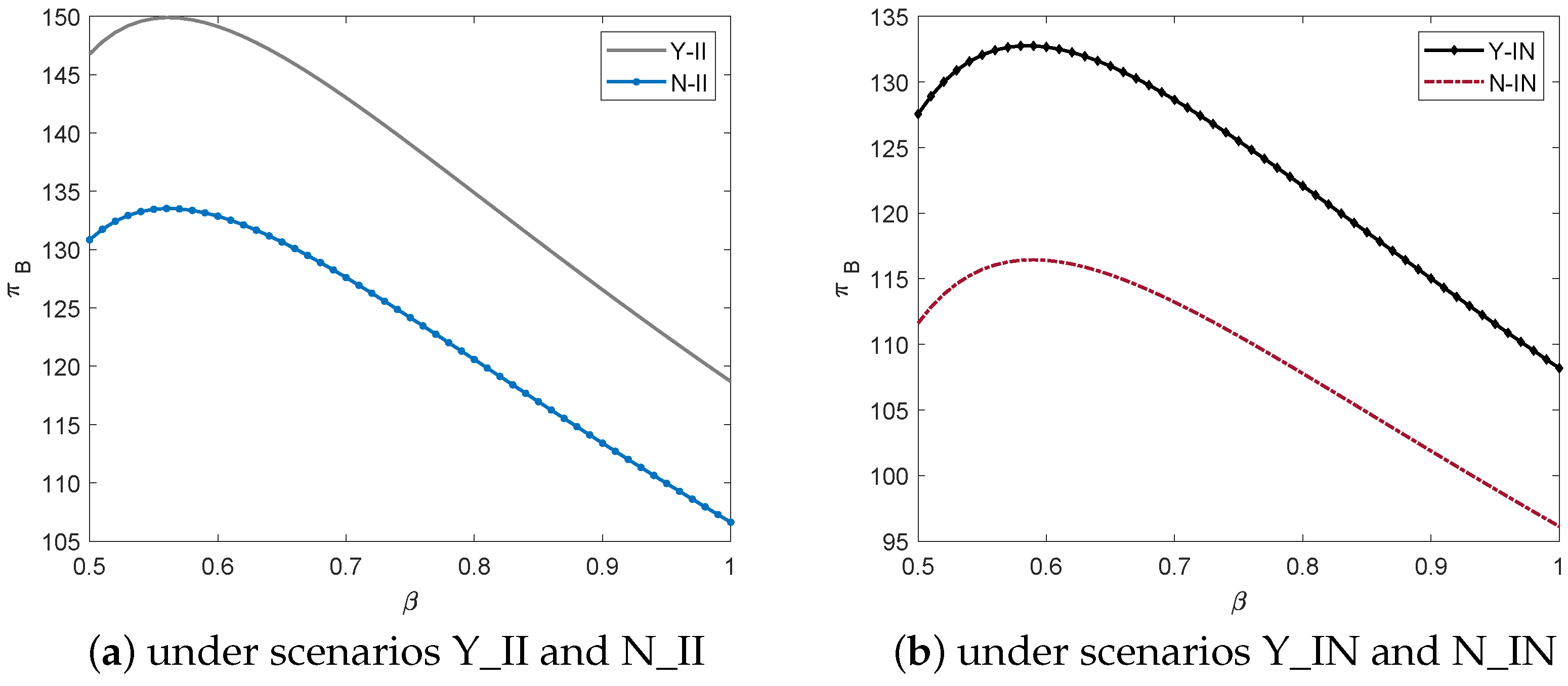
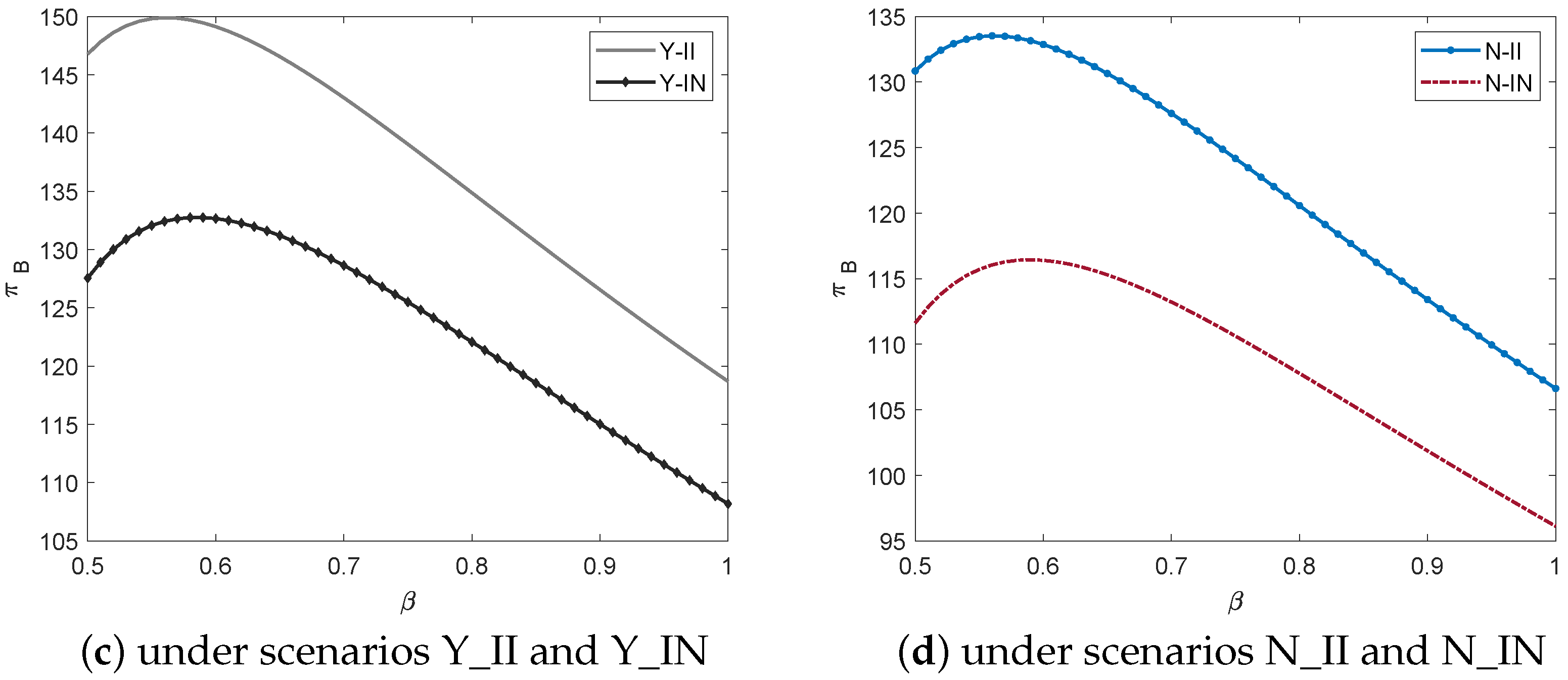
4.1. Profit Analysis for Retailers

With the guarantee that all variables are positive, the relevant parameters can be set as initial market potential $a=30$, information purchase fee and compensation fee $F=20$, unit shipping fee charged by the carrier to retailers ${\omega }_0=5$, unit shipping fee charged by the carrier to overseas customers ${\omega }_1=6$, the commission rate charged by the platform $\eta =0.02$, forecast of market demand $E\left[\epsilon \right|\mathrm{\Gamma }]=10$ and price sensitivity to its own quantity $\beta =1$. Since $\beta$ is set to be greater than $\gamma$, we let price sensitivity to its rivals’ quantity $\gamma =0.4$, and the value range of price sensitivity to its own quantity $\beta$ can be limited to the range $[0.5,1]$.

Figure 3a shows retailer A can obtain the biggest profit when retailer B obtains the information and chooses the strategy of no free shipping. Moreover, retailer A has a larger profit when retailer B obtains the information regardless of whether retailer B chooses free shipping. However, from Figure 3b, retailer B’s profit from offering free shipping is always greater than the profit from not offering, regardless of whether it gets information. Therefore, retailer B prefers to provide free shipping services. Concerning retailer B’s willingness to obtain the information, we find that when the information purchase fee $F=20$, $\beta$ is located in area a, whether or not free shipping is chosen, the profit when retailer B gets the information is always greater than the profit when it does not. However, when the price has a great influence on its own quantity, that is, $\beta$ is located in area b, retailer B will choose not to buy the information. We can speculate that retailer B is willing to spend a higher information cost to purchase information when the degree of necessity of the product is more elevated.

We can see that retailer B is uncertain about whether to purchase information when the information purchase fee is large. Proposition 4 states that the information purchase fee has a greater impact on retailer B’s decision to purchase information. We change the fee of purchasing information to $F=5$, and obtain Figure 4. As shown from Figure 4a,b, regardless of whether retailer B chooses free shipping, the profit of obtaining information is always greater than that of not obtaining information. Therefore, when the information purchase fee is small, retailer B ignores the effect of product necessity and purchases the information. Moreover, reducing the information purchase fee does not affect retailer B’s choice of free shipping decision (see Figure 4c,d). From this, we can see that the information purchase fee has an important influence on retailer B’s decision on whether to buy the information. That is, when the price is more sensitive to its own quantity (the necessity of the product is low), the platform needs to control the information purchase fee to enable information sharing.

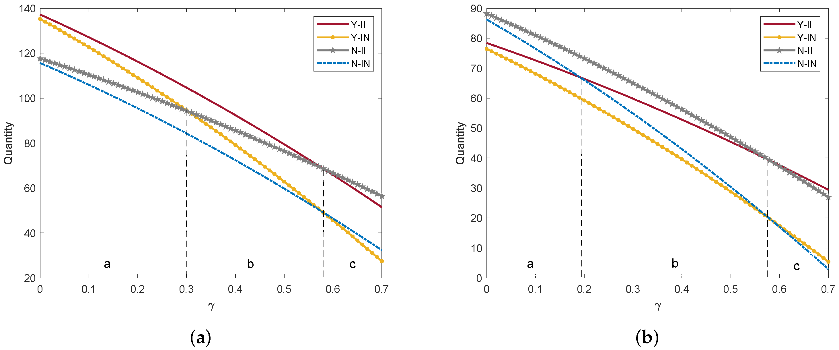
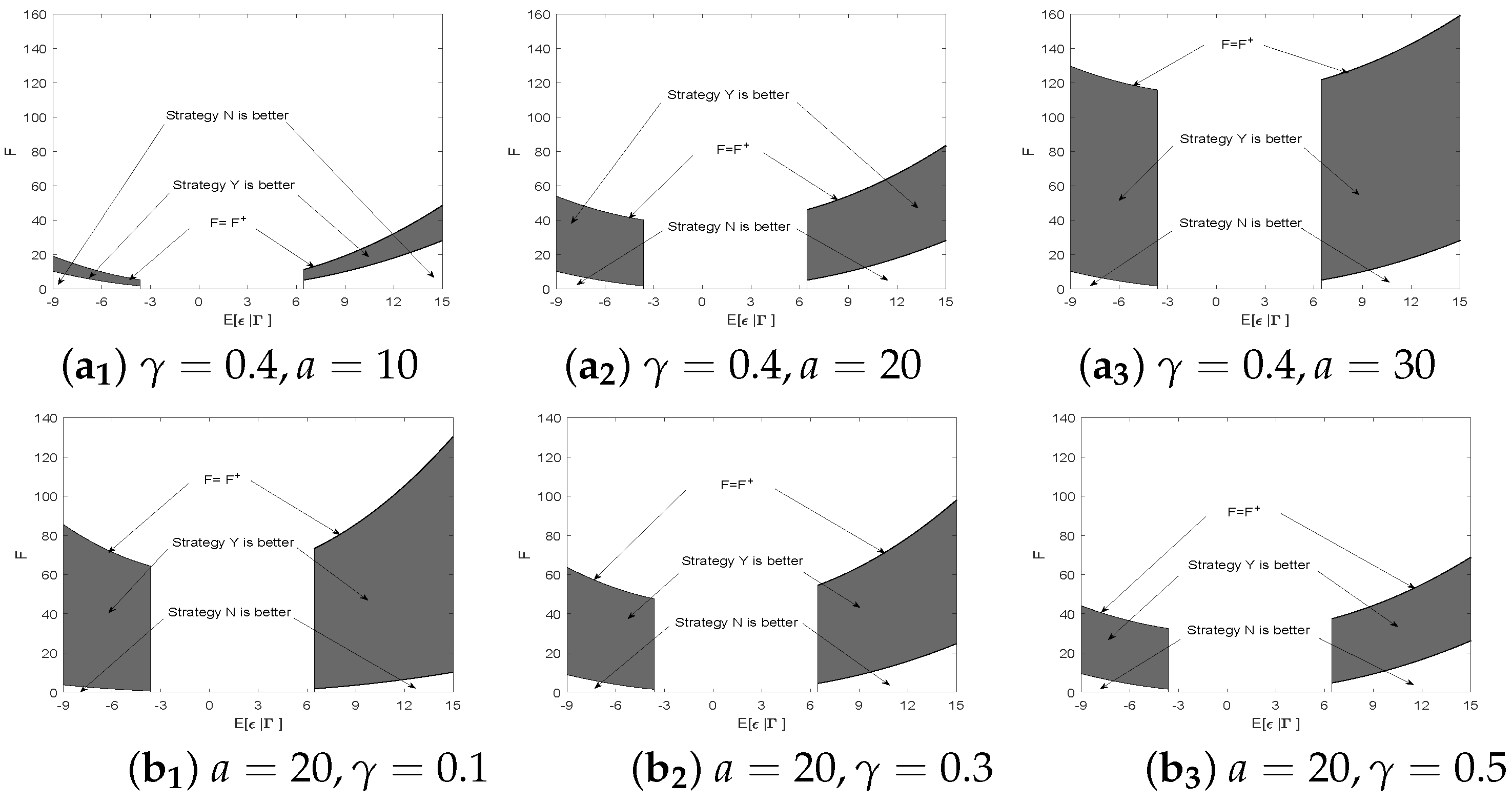
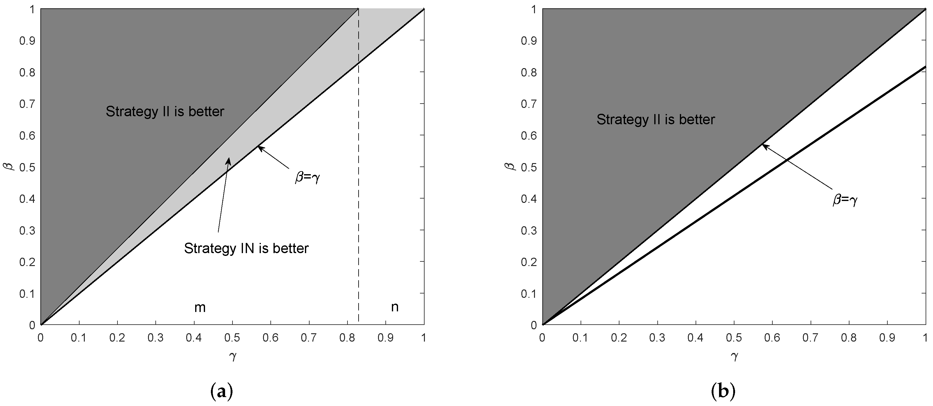
4.2. Strategic Choices for Retailers

We observe the effects of initial market potential and competitive intensity on retailer A’s willingness to share information, and draw Figure 5. We define the value ranges of $E\left[\epsilon \right|\mathrm{\Gamma }]$ and F in the graph to ensure that all variables are positive. Let $F<\frac{(1-\eta )\left(a\left(4{\beta }^2-2\beta \gamma -{\gamma }^2\right)+{\omega }_1\left({\gamma }^2-4{\beta }^2\right)+2\beta \gamma {\omega }_0\right){}^2}{16\beta {\left({\gamma }^2-2{\beta }^2\right)}^2}+\frac{(1-\eta ){\left(-4{\beta }^2+2\beta \gamma +{\gamma }^2\right)}^2}{16\beta {\left({\gamma }^2-2{\beta }^2\right)}^2}\times \frac{{\sigma }^4}{{\sigma }^2+{\sigma }_1^2}=F^{+}$, and draw the maximum value of F desirable in the graph. Consistent with the above variable settings, let the unit shipping fee charged by the carrier to retailers remain ${\omega }_0=5$, the unit shipping fee charged to overseas customers ${\omega }_1=6$, the commission rate charged by the platform $\eta =0.02$, and let price sensitivity to its own quantity $\beta =0.7$.

We observe the effect of initial potential changes in the market and changes in competitive intensity on the strategic choices of retailers A (see Figure 5). The greater the initial market potential, the greater the incentive for retailer A to share information. However, the effect of competition intensity on retailer A’s desire to share information is negative, the bigger the competition intensity, the less retailer A’s incentive to share information desire.

Next, we analyze retailer B’s free shipping strategy. With ${\omega }_0=5$, ${\omega }_1=6$, $1\ge \beta >\gamma >0$, according to Proposition 4 (b${}_3$–b${}_4$), we analyze the cases of $a<K_3$ and $a>K_3$ separately. In the range of definition, we let $a=6$ and $a=30$, respectively. Under the basic assumption that $\beta >\gamma$ is satisfied, we analyze retailer B’s preference by drawing Figure 6. It shows retailer B’s choice of free shipping strategy. We find that the probability of retailer B choosing free shipping is greater than the probability of selecting no free shipping when the initial market potential $a<K_3$. And when the competitive intensity of the market $\gamma$ is located in area m, the probability of retailer B choosing not to have free shipping increases with the competitive intensity. Still, when the competitive intensity is greater ($\gamma$ is located in area n), retailer B only chooses no free shipping.

When the initial market potential $a>K_3$, the shape of the graph remains the same regardless of the change in parameters, so retailer B always chooses the free shipping strategy. The possible reason is that when the initial market potential is small, retailer B has just entered the market and is less competitive. Faced with greater competitive pressure, retailer B is unwilling to risk high shipping fees. However, when the initial market potential is larger, the advantage of free shipping will increase the demand quantities, and then retailer B will choose to offer free shipping to be more competitive and maximize its profit.

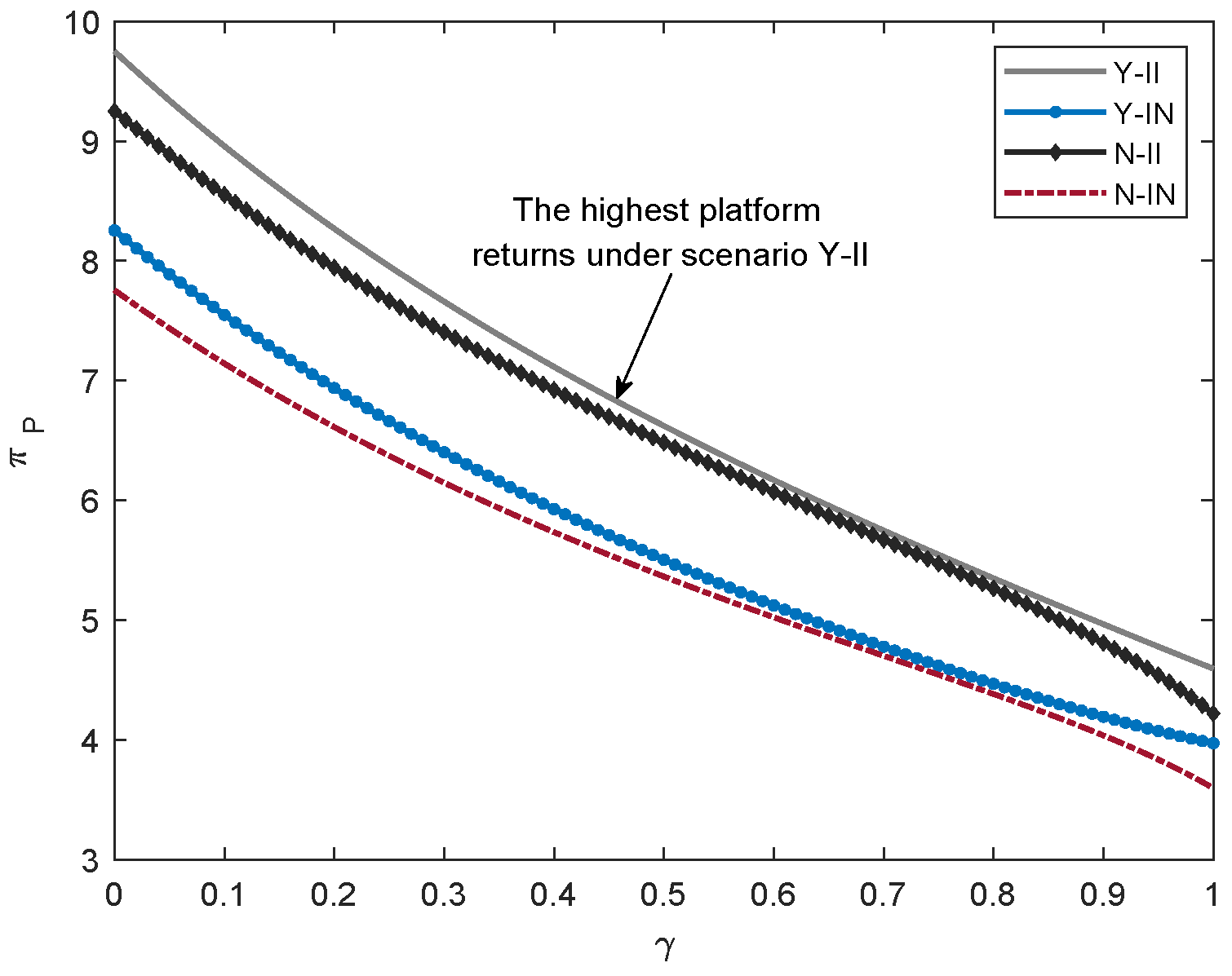
4.3. Platform Numerical Analysis

The number of sales on the platform is an essential indicator of e-commerce platform operations. To analyze the impact of market competition on the overall number of platform sales under different market forecasts, we set basic market potential $a=30$, price sensitivity to its own quantity $\beta =1$, unit shipping fee charged by the carrier to retailers ${\omega }_0=5$, unit shipping fee charged by the carrier to overseas customers ${\omega }_1=6$, and when the market demand forecast is positive, predicted value $E\left[\epsilon \right|\mathrm{\Gamma }]=10$, when it is negative, predicted value $E\left[\epsilon \right|\mathrm{\Gamma }]=-5$. The intensity of market competition $\gamma$ can be limited to a range $(0,0.7)$. Add the equilibrium quantities of retailers A and B in each case, $Q=q_A^{\mathrm{i}\_\mathrm{Ij}}+q_B^{\mathrm{i}\_\mathrm{Ij}}$, where $i\in [Y,N]$, $j\in [I,N]$. Substituting the above parameters into Q. As $\gamma$ increases gradually in the range of values, the total number of sales will change accordingly. We compare the total number of deals on the platform in four cases. To observe the law of substantial change, the results are mapped to graphs to analyze the influence of competition intensity on the total number of sales under different market forecasts.

From Figure 7, we can see that the overall number of sales on the platform decreases as the intensity of competition increases. Further, the number of sales is greater when the forecast for the market is positive than when it is negative. Figure 7a shows the results for an uncertain market with a positive demand forecast. While the market competition is small ($\gamma$ is located in area a), the total number of sales on the platform at the time retailer B obtains the information is greater. When the competition intensity is in the middle region ($\gamma$ is located in area b), the platform has a greater total number of sales when retailer B chooses free shipping. And when the market competition is strong ($\gamma$ is located in area c), the platform’s total number of sales when retailer B chooses free shipping is still greater than when shipping is not free. Still, the platform’s total number of sales is larger when retailer B does not obtain the information. This is because, under fierce competition, retailer B will reduce its quantitative decisions based on the principle of risk aversion if market demand information is known. Figure 7b shows the results when the market demand forecast is negative. Interestingly, when there is less competition, the platform sells more when retailer B does not obtain the information. The reason is that here the market demand forecast for uncertainty is negative. After getting information, retailer B naturally makes fewer quantitative decisions. However, when the competitive pressure is particularly high ($\gamma$ is located in the c area), the total platform sales are greater at the time retailer B gets the information. The possible reason for this is that retailer A will reduce its quantitative decision when faced with greater market pressure and a negative market forecast. Under the Stackelberg game, retailer B’s quantitative decision will decrease with retailer A. If retailer B knows the demand information, it may increase part of the quantitative decision when retailer A reduces.

The intensity of market competition has a significant impact on the total number of transactions on the platform, and we further analyze the impact of market competition intensity on platform profits. We plot the profits of the platform in different scenarios under the market mode in Figure 8. Because the profits of the platform are drawn from the profits of retailers A and B, analyzing the profits of retailers A and B in Figure 3 together, we find that although the profits of retailer A are the largest in scenario Y_IN, the profits of the platform are the same as the profit profile of retailer B, which is larger in scenario Y_II. To achieve a win–win situation for all parties, the platform needs to develop appropriate operational strategies to influence factors such as initial market potential and market competition intensity, thus indirectly intervening in the strategic choices of retailers.

5. Discussion and Conclusions

It is crucial to consider how to operate the CBEC platform supply chain with long distances and high costs. We investigated the decision-making of retailers on CBEC platforms regarding information sharing and free shipping under the marketplace mode, and we examined the willingness of information sharing between the existing retailer and the new entrant retailers. The results obtained using theoretical and numerical analysis show that:

(1) In terms of the information-sharing strategy, we find that the existing retailer’s willingness to share information is influenced by initial market potential and competitive intensity. The effect of initial market potential on the willingness to share information is positive. As the initial market potential increases, the willingness of existing retailers to share information also increases. In contrast, the effect of market competition intensity on willingness to share information is negative, i.e., as competition intensity increases, the willingness of existing retailers to share information decreases. The existing retailer will share information when the initial market potential is larger, and the intensity of competition in the market is smaller. In addition, the information fee greatly influences the existing retailer’s willingness to share information and the willingness of the new retailer to acquire information. Information sharing can only be realized when the information fee meets certain conditions.

(2) In terms of the free shipping strategy, we find that both initial market potential and competitive intensity affect the choice of the new entrant retailer. When the initial market potential is larger, the new entrant retailer always chooses the free shipping strategy. However, when the initial market potential is smaller, the willingness to choose free shipping decreases as competition intensifies. And when the market tends to be perfectly competitive, the new entrant retailer will decide not to offer free shipping. It is worth noting that if the existing retailer offers free shipping, information sharing will not affect the retailer’s free shipping decision in a healthy competitive market environment. The new entrant will always offer free shipping, which is consistent with reality.

From the platform perspective, it is clear that the platform is most profitable when information sharing and free shipping occur simultaneously. For information sharing and free shipping to co-occur, the platform needs to set up reasonable operational strategies to meet the following conditions: the larger initial market potential, the smaller market competition intensity, and the reasonable information fee. Therefore, the platform could seize market share with other platforms by increasing advertising, improving service levels, and enriching products to increase initial market potential and reduce market competition intensity; it can also control the number of e-retailers on the platform and reduce market competition intensity. In addition, while maintaining product diversification, the platform should also consider the attributes of products sold by retailers. When the necessity of the product is higher, the new entrant retailer is willing to spend a higher information cost to purchase information.

The obtained results enrich the theoretical results of platform supply chains by starting from information sharing and free shipping strategies. However, there are still limitations in this paper. First, we set the shipping fee as an exogenous variable that is not generalizable. We consider setting the shipping fee as a decision variable in future studies and considering shipping fee discounts. Second, the service quality of transportation is also a vital issue in CBEC. In the future, we will discuss the competition among retailers by considering the quality of shipping service when free shipping is available. Finally, tax differences are prominent features of cross-border e-commerce. In the future, we will study the competition in the supply chain of B2B e-commerce platforms based on tax planning.

References

1. Awiagah, R.; Kang, J.; Lim, J.I. Factors affecting e-commerce adoption among SMEs in Ghana. Inf. Dev. 2016, 32, 815–836. [Google Scholar] [CrossRef]
2. Alzahrani, J. The impact of e-commerce adoption on business strategy in Saudi Arabian small and medium enterprises (SMEs). Rev. Econ. Polit. Sci. 2019, 4, 73–88. [Google Scholar] [CrossRef]
3. Wang, J. Opportunities and challenges of international e-commerce in the pilot areas of China. Int. J. Mark. Stud. 2014, 6, 141. [Google Scholar] [CrossRef]
4. Baek, E.; Lee, H.K.; Choo, H.J. Cross-border online shopping experiences of Chinese shoppers. Asia Pac. J. Mark. Logist. 2019, 32, 366–385. [Google Scholar] [CrossRef]
5. Hadasik, B.; Kubiczek, J. E-commerce market environment formed by the COVID-19 pandemic—A strategic analysis. Forum Sci. Oecon. 2022, 10, 25–52. [Google Scholar]
6. Adam, I.O.; Alhassan, M.D.; Afriyie, Y. What drives global B2C E-commerce? An analysis of the effect of ICT access, human resource development and regulatory environment. Technol. Anal. Strateg. Manag. 2020, 32, 835–850. [Google Scholar] [CrossRef]
7. Hua, G.; Wang, S.; Cheng, T. Optimal order lot sizing and pricing with free shipping. Eur. J. Oper. Res. 2012, 218, 435–441. [Google Scholar] [CrossRef]
8. Shehu, E.; Papies, D.; Neslin, S.A. Free shipping promotions and product returns. J. Mark. Res. 2020, 57, 640–658. [Google Scholar] [CrossRef]
9. Niu, B.; Xu, H.; Xie, F. Free shipping in cross-border supply chains considering tax disparity and carrier’s pricing decisions. Transp. Res. Part. Logist. Transp. Rev. 2021, 152, 102369. [Google Scholar] [CrossRef]
10. Song, Y.; Liu, J.; Zhang, W.; Li, J. Blockchains role in e-commerce sellers decision-making on information disclosure under competition. Ann. Oper. Res. 2022, 1–40. [Google Scholar] [CrossRef]
11. Qu, S.; Xu, L.; Mangla, S.K.; Chan, F.T.; Zhu, J.; Arisian, S. Matchmaking in reward-based crowdfunding platforms: A hybrid machine learning approach. Int. J. Prod. Res. 2022, 60, 7551–7571. [Google Scholar] [CrossRef]
12. Qu, S.; Li, Y.; Ji, Y. The mixed integer robust maximum expert consensus models for large-scale GDM under uncertainty circumstances. Appl. Soft Comput. 2021, 107, 107369. [Google Scholar] [CrossRef]
13. Dominguez, R.; Cannella, S.; Barbosa-Póvoa, A.P.; Framinan, J.M. OVAP: A strategy to implement partial information sharing among supply chain retailers. Transp. Res. Part. Logist. Transp. Rev. 2018, 110, 122–136. [Google Scholar] [CrossRef]
14. Lv, Q. Supply chain decision-making of cross-border E-commerce platforms. Adv. Ind. Eng. Manag. 2018, 7, 1–5. [Google Scholar]
15. Lu, Y.H.; Yeh, C.C.; Liau, T.W. Exploring the key factors affecting the usage intention for cross-border e-commerce platforms based on DEMATEL and EDAS method. Electron. Commer. Res. 2022, 1–23. [Google Scholar] [CrossRef]
16. Zha, X.; Zhang, X.; Liu, Y.; Dan, B. Bonded-warehouse or direct-mail? Logistics mode choice in a cross-border e-commerce supply chain with platform information sharing. Electron. Commer. Res. Appl. 2022, 54, 101181. [Google Scholar] [CrossRef]
17. Qi, X.; Chan, J.H.; Hu, J.; Li, Y. Motivations for selecting cross-border e-commerce as a foreign market entry mode. Ind. Mark. Manag. 2020, 89, 50–60. [Google Scholar] [CrossRef]
18. Cao, K.; Xu, Y.; Cao, J.; Xu, B.; Wang, J. Whether a retailer should enter an e-commerce platform taking into account consumer returns. Int. Trans. Oper. Res. 2020, 27, 2878–2898. [Google Scholar] [CrossRef]
19. Jiang, B.; Jerath, K.; Srinivasan, K. Firm strategies in the mid tail of platform-based retailing. Mark. Sci. 2011, 30, 757–775. [Google Scholar] [CrossRef]
20. Li, C.; Chu, M.; Zhou, C.; Xie, W. Is it always advantageous to add-on item recommendation service with a contingent free shipping policy in platform retailing? Electron. Commer. Res. Appl. 2019, 37, 100883. [Google Scholar] [CrossRef]
21. Wang, Y.Y.; Li, J. Research on pricing, service and logistic decision-making of E-supply chain with Free Shipping strategy. J. Control Decis. 2018, 5, 319–337. [Google Scholar] [CrossRef]
22. Han, S.; Chen, S.; Yang, K.; Li, H.; Yang, F.; Luo, Z. Free shipping policy for imported cross-border e-commerce platforms. Ann. Oper. Res. 2022, 1–30. [Google Scholar] [CrossRef]
23. Etumnu, C.E. Free shipping. Appl. Econ. Lett. 2022, 1–4. [Google Scholar] [CrossRef]
24. Leng, M.; Becerril-Arreola, R. Joint pricing and contingent free-shipping decisions in B2C transactions. Prod. Oper. Manag. 2010, 19, 390–405. [Google Scholar] [CrossRef]
25. Rui, G.; XiaXia, M.; TianXing, S. Research on the Impact of Consumers—Time Sensitivity on E-commerce Free Shipping Strategy. In Proceedings of the 2020 Chinese Control And Decision Conference (CCDC), Hefei, China, 22–24 August 2020; pp. 4204–4209. [Google Scholar]
26. Li, L.; Zhang, H. Confidentiality and information sharing in supply chain coordination. Manag. Sci. 2008, 54, 1467–1481. [Google Scholar] [CrossRef]
27. Jain, A.; Seshadri, S.; Sohoni, M. Differential pricing for information sharing under competition. Prod. Oper. Manag. 2011, 20, 235–252. [Google Scholar] [CrossRef]
28. Ha, A.Y.; Tong, S.; Zhang, H. Sharing demand information in competing supply chains with production diseconomies. Manag. Sci. 2011, 57, 566–581. [Google Scholar] [CrossRef]
29. Shang, W.; Ha, A.Y.; Tong, S. Information sharing in a supply chain with a common retailer. Manag. Sci. 2016, 62, 245–263. [Google Scholar] [CrossRef]
30. Huang, S.; Guan, X.; Chen, Y.J. Retailer information sharing with supplier encroachment. Prod. Oper. Manag. 2018, 27, 1133–1147. [Google Scholar] [CrossRef]
31. Min, Z.; Mikai, X.; Debao, D. Research on game strategy of information sharing in cross-border e-commerce supply chain between manufacturers and retailers. In Proceedings of the Advances in Intelligent Systems and Interactive Applications, Proceedings of the 4th International Conference on Intelligent, Interactive Systems and Applications (IISA2019), Bangkok, Thailand, 28–30 June 2019; Springer: Berlin/Heidelberg, Germany, 2020; pp. 399–406. [Google Scholar]
32. Kirby, A.J. Trade associations as information exchange mechanisms. Rand J. Econ. 1988, 19, 138–146. [Google Scholar] [CrossRef]
33. Niu, B.; Dai, Z.; Chen, L. Information leakage in a cross-border logistics supply chain considering demand uncertainty and signal inference. Ann. Oper. Res. 2022, 309, 785–816. [Google Scholar] [CrossRef]
34. Liu, Z.; Zhang, D.J.; Zhang, F. Information sharing on retail platforms. Manuf. Serv. Oper. Manag. 2021, 23, 606–619. [Google Scholar] [CrossRef]
35. Mukhopadhyay, S.K.; Yue, X.; Zhu, X. A Stackelberg model of pricing of complementary goods under information asymmetry. Int. J. Prod. Econ. 2011, 134, 424–433. [Google Scholar] [CrossRef]
36. Xu, X.; Chen, Y.; He, P.; Yu, Y.; Bi, G. The selection of marketplace mode and reselling mode with demand disruptions under cap-and-trade regulation. Int. J. Prod. Res. 2021, 1–20. [Google Scholar] [CrossRef]
37. Simon, D.; Fischbach, K.; Schoder, D. Enterprise architecture management and its role in corporate strategic management. Inf. Syst. Bus. Manag. 2014, 12, 5–42. [Google Scholar] [CrossRef]
38. Qu, S.; Shu, L.; Yao, J. Optimal pricing and service level in supply chain considering misreport behavior and fairness concern. Comput. Ind. Eng. 2022, 174, 108759. [Google Scholar] [CrossRef]
39. Bai, Q.; Xu, J.; Gong, Y.; Chauhan, S.S. Robust decisions for regulated sustainable manufacturing with partial demand information: Mandatory emission capacity versus emission tax. Eur. J. Oper. Res. 2022, 298, 874–893. [Google Scholar] [CrossRef]
40. Niu, B.; Dai, Z.; Zhuo, X. Co-opetition effect of promised-delivery-time sensitive demand on air cargo carriers—Big data investment and demand signal sharing decisions. Transp. Res. Part. Logist. Transp. Rev. 2019, 123, 29–44. [Google Scholar] [CrossRef]
41. Xing, W.; Li, Q.; Zhao, X.; Li, J. Information sale and contract selection under downstream competition. Transp. Res. Part. Logist. Transp. Rev. 2020, 136, 101870. [Google Scholar] [CrossRef]
42. Singh, N.; Vives, X. Price and quantity competition in a differentiated duopoly. Rand J. Econ. 1984, 15, 546–554. [Google Scholar] [CrossRef]
43. Roy, R.A. Market Information and Firm Performance. Manag. Sci. 2000, 46, 1075–1084. [Google Scholar]
44. Bai, Q.; Xu, J.; Chauhan, S.S. Effects of sustainability investment and risk aversion on a two-stage supply chain coordination under a carbon tax policy. Comput. Ind. Eng. 2020, 142, 106324. [Google Scholar] [CrossRef]
Figure 1. Supply chain structure.
Sustainability 15 03350 g001
Figure 2. Sequence of events.
Sustainability 15 03350 g002
Figure 3. The changes in retailer A and B’s profit with respect to β under four scenarios. (a) Retailer A. (b) Retailer B.
Sustainability 15 03350 g003
Figure 4. Profits comparison of retailer B under different scenarios ( F = 5 ).
Sustainability 15 03350 g004aSustainability 15 03350 g004b
Figure 5. Retailer A’s preference over sharing information strategy.
Sustainability 15 03350 g005
Figure 6. Retailer B’s preference over free shipping strategy. (a) a < K 3 . (b) a > K 3 .
Sustainability 15 03350 g006
Figure 7. The size of overseas market comparison of four scenarios under different market forecasts. (a) ( ε + ε 1 ) > 0 . (b) ( ε + ε 1 ) < 0 .
Sustainability 15 03350 g007
Figure 8. Profit comparison of platform P under four scenarios.
Sustainability 15 03350 g008