An Autonomous Marine Mucilage Monitoring System

Abstract

Mucilage bloom is a current issue, especially for countries in the Mediterranean Basin, due to economic activities and ecological effects. The main causes are increased nutrient load due to organic and industrial pollution in the sea, global warming, and meteorological conditions at a level that can trigger mucilage bloom. It is important to take permanent measures to combat the increased nutrient load causing mucilage. However, there are various actions that can be performed during the mucilage bloom period, especially the collection of mucilage on the sea surface. Surface vehicles can be used to monitor and collect mucilage on the sea surface. The aim of this study is to design an autonomous marine mucilage monitoring system for systems such as unmanned surface vehicles (USV). We suggest monitoring the risky Marmara Sea continuously and recording some of the key parameters using a USV. The onboard solution proposed in this study has an architect based on a three-tier mucilage monitoring system. In the first tier, the sea surface is scanned with camera(s) in a certain radius in real time. When mucilage-candidate areas are determined, the vehicle is directed to this region autonomously. In the second tier, seawater in the region is measured in real time with some onboard sensors, pH level, conductivity, and dissolved oxygen level. The third tier is where real samples at three different depths are collected (if possible) for detailed posterior lab analysis. We have compared image processing, CNN (ResNet50), kNN, SVM, and FFNN approaches and have shown that the accuracy of our proposed mucilage classification method offers better and more promising performance.

1. Introduction

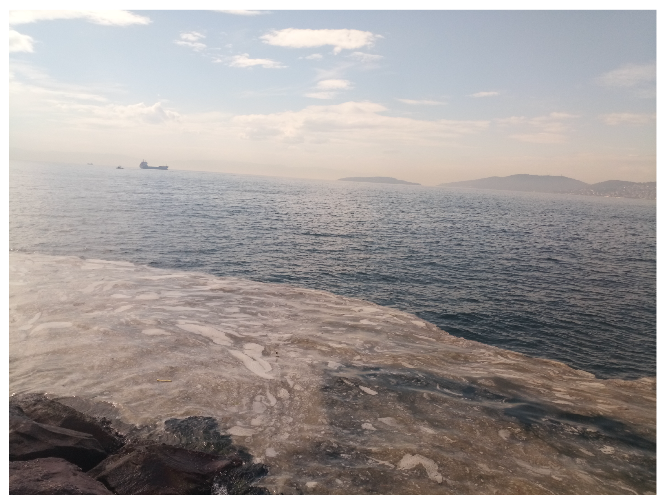
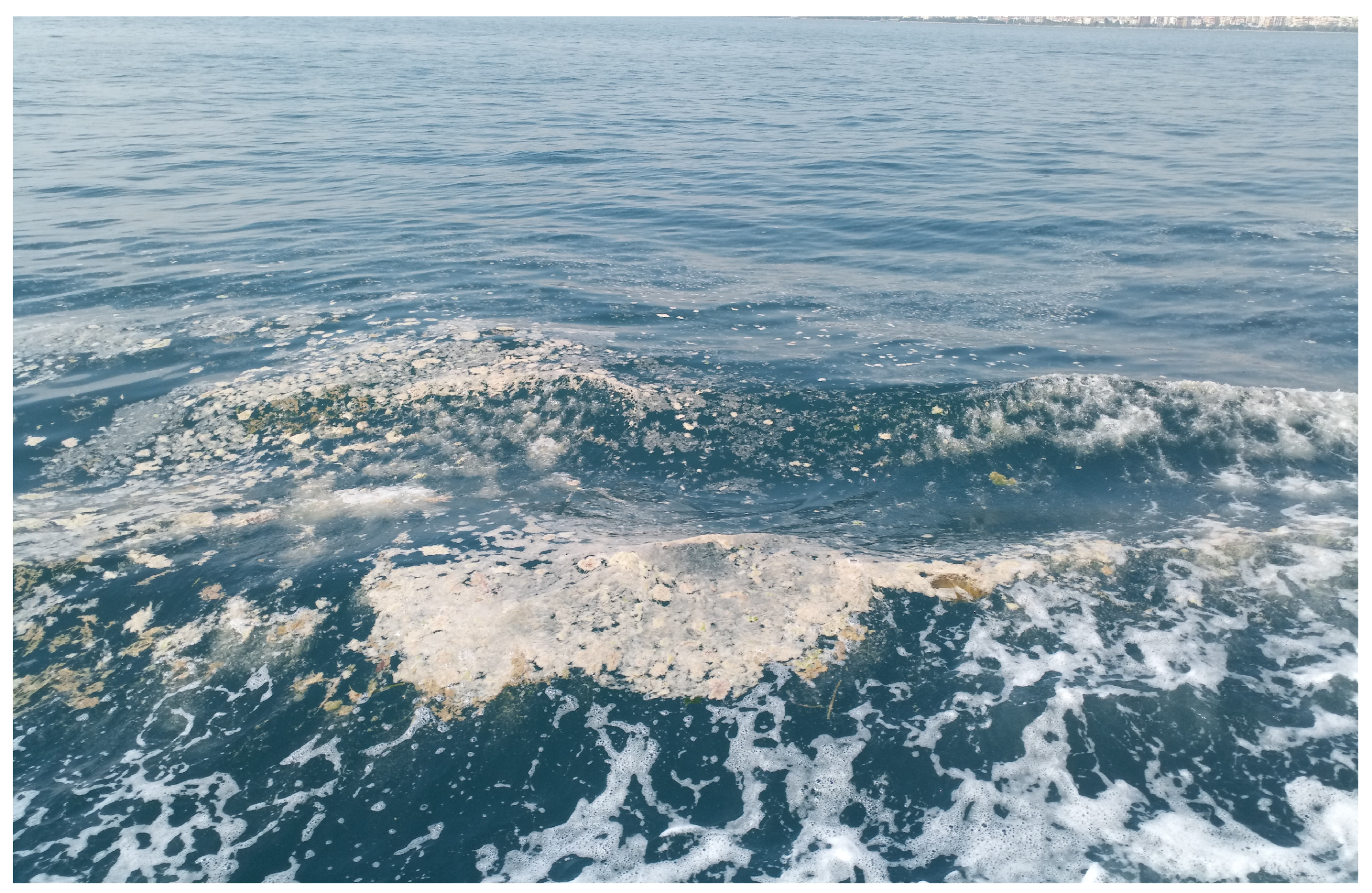
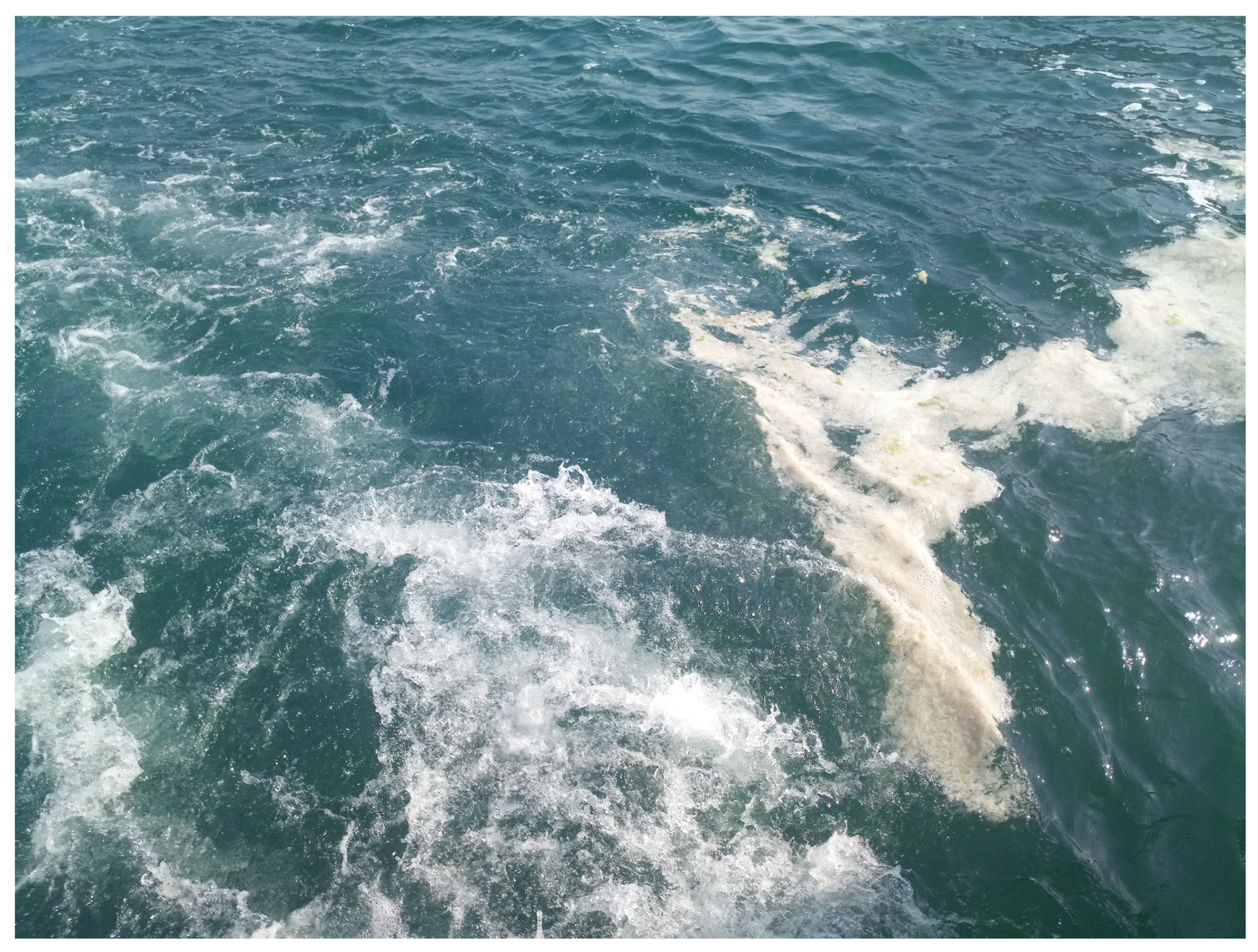
Mucilage is a phenomenon that is caused by several different macro-aggregates. Marine snow and sea snow terms are also used for marine mucilage. Although it is sometimes only possible to observe mucilage in deep water, it is also observed on the sea’s surface very often as creamy or gelatinous substances [1]. An example of creamy marine mucilage is given in Figure 1, and an example of gelatinous marine mucilage is given in Figure 2. The area of each mucilage part on the sea’s surface can exhibit different sizes within a wide range. The small mucilage parts can be observed frequently on sea surfaces; however, the large ones can be observed at the time of mucilage bloom [1]. Nevertheless, mucilage is a phenomenon of nature. There are some factors that increase the volume of mucilage, such as high levels of industrialization, the increase in the usage of agricultural chemicals, a substantial amount of fishing, and a high volume of marine traffic. If the conditions are met, factors such as increasing temperatures or a change in wind speed can provoke a mucilage bloom [1]. In the study of Komuscu et al. [2], it has also been shown in detail that mucilage cannot be explained only by a change in meteorological conditions, but a combination of other environmental factors and meteorological conditions can cause the phenomenon of mucilage bloom [2].

There are several studies that monitor sea surfaces. Satellite-based data were used in some of these studies [3,4,5,6,7,8,9,10]. Rasuly et al. [3] examined satellite images of the Caspian Sea’s coasts in their study. The authors proposed a method to determine the changes in the water level on the coasts by evaluating satellite images [3]. Bondur et al. [4] examined anthropogenic influences in the Mamola Bay region of Hawaii, USA, using sensor data from different satellites [4]. Messager et al. [5] performed ocean monitoring using synthetic aperture radar (SAR) data. One of the aims of the study targeted oil spill detection. A support vector machine (SVM)-based classification has also been utilized for this process [5]. Ferreira et al. [6] used satellite data to monitor chlorophyll-a concentrations in the Western Antarctic Peninsula. The authors proposed a custom algorithm and used machine learning methods for this purpose [6]. Khan et al. [7] investigated satellite data to monitor glaciers. They used SVM, ANN, and RF methods and compared the success of these methods to their application [7]. Shen et al. [8] used satellite data to classify sea ice types. CNN, k-nearest neighbor (kNN), and SVM are some of the methods used for this purpose. The accuracy rates of the different methods used are provided comparatively [8]. Gokaraju et al. [9] proposed a method that monitors harmful algal blooms in the US Gulf of Mexico region using satellite-based sensor data. For this purpose, an SVM-based method was developed [9]. Hereher investigated a system that monitors sea surface temperatures using satellite image data [10]. There are also studies aiming to monitor marine mucilage, one of the sea’s surface irregularities, using satellite data. Kavzoglu et al. [11] investigated a method for describing mucilage areas using satellite-based photos. A random-forest-based method was used to detect mucilage areas. The authors focused on finding differences in the patterns on the sea’s surface due to the ship’s movements and marine mucilage [11]. Yagci et al. [1] also determined whether there was mucilage by using satellite images. In the method they used, they made use of moderate-resolution imaging spectroradiometer (MODIS) products that contained satellite images. A mucilage index was created by using the green and blue pixel values of the sea images and the near-infrared (NIR) and short-wave infrared (SWIR) values. The algorithm decides whether mucilage is present or not by performing evaluations according to this index using the data coming from the satellite’s images [1]. In the study of Cavalli [12], MODIS was also used. In that study, sea surface temperatures were calculated using MODIS data [12]. Acar et al. [13] used image data taken from satellites to monitor marine mucilage. Satellite data were retrieved from the Google Earth Engine. Firstly, the authors used several indexes in order to mask clouds, such as the normalized difference vegetation index (NDVI) and normalized difference water index (NDWI). After that, the median filter was applied to the images. Using a supervised random forest (RF) classifier, the mucilage and non-mucilage areas on the sea’s surface were detected [13]. Another study that focused on marine mucilage detection using satellite data was presented by Tassan [14]. In his work, the data of satellite-based and advanced very high-resolution radiometers (AVHRR) were used to monitor floating mucilage parts on sea surfaces [14].

Utilizing unmanned aerial vehicles is also a common method for detecting irregularities on the sea’s surface and beaches. Pinto et al. [15] attempted to detect pollution on Portuguese beaches. In the aforementioned study, the areas that are contaminated with large-scale objects on the beach were determined by using different machine learning methods, which were classified according to their types. The authors added that one of the aims of the study was to accurately direct cleaning personnel on beaches [15]. Goncalves et al. [16] collected images from Portuguese beaches in their study and investigated the observed pollution elements in the images. This study also included contamination detection with machine learning methods compared with manual contamination detection using operators. CNN and RF methods were used as the machine-learning methods. The authors proposed that machine-learning methods would yield better results when the database grew and when the number of these types of studies increased [16]. Goncalves et al. [17] examined unmanned aerial vehicle images that they took from the Portuguese beaches in their study. In the obtained data, they attempted to detect polluted areas by using three different object-oriented machine learning methods, namely kNN, SVM, and RF. In their comparison, the RF method produced more successful results among these three methods. It has been emphasized that the kNN method is an effective method for non-experts due to its simplicity [17]. Fallati et al. [18] applied CNN-based deep learning methods in their study. The images were obtained by using unmanned aerial vehicles over the beaches of the Republic of Maldives. In that study, the researchers also classified identified pollutants according to their types [18]. One of the problems that have increased in recent years and threaten both nature and the economy is the jellyfish problem [19]. Kim et al. [20] monitored jellyfish in the images obtained from unmanned aerial vehicles using CNN-based classifiers. The authors stated that they achieved accuracy values over 80 percent [20]. Narmillan et al. [21]. investigated UAV multispectral images to monitor fields. The success of different machine learning methods was compared to find the best accuracy [21]. Goncalves et al. [22] aimed to obtain three-dimensional image data of coastal areas in their study. The main motivation of their study was to determine the maintenance needs of rocky coastal groins. For this purpose, both UAV and terrestrial laser scanning (TLS) systems were used, and the success rates of these systems were compared [22]. There is also a study that used UAVs to image phaeocystis globosa algal bloom, which exhibits a gelatinous appearance that is similar to the mucilage that it can take on from time to time [23]. Using hyperspectral imaging, regions of high algal bloom were identified by UAVs [23]. Manned aerial vehicles were also used to monitor marine mucilage. Zambianchi et al. [24] monitored marine mucilage on sea surfaces using manned aircraft to classify regions as those with mucilage and those without mucilage. Red, green, and blue (RGB)-based thresholding algorithms were used [24].

Unmanned/manned surface vehicles are commonly used for marine fauna monitoring [25,26]. Tian et al. [27] observed sea ice with the data they collected from the boat in their study. Since the detections made with the naked eye take a long time and are expensive, the authors have developed an algorithm to automate this task. Images taken from the surface vehicle have benefited from methods such as support vector machine (SVM) and random forest (RF), and they achieved successful results over four out of five. It was stated by the authors that this rate increased with the addition of different machine learning methods [27]. Cao et al. [28] investigated an USV to monitor quality of sea water. Data of total dissolved solids, pH and turbidity are used to decide the quality of water in that study [28]. Dabrowski et al. [29] processed data, taken from satellite, unmanned aerial vehicle (UAV) and USV together and observed the tombolo phenomenon in Sopot, Poland [29]. Specht et al. [30] investigated a bathymetric monitoring system for shallow waterbodies. Both UAV and USV are used in that system. For data processing several methods including artificial neural networks (ANN) are used [30]. Papachristopoulou et al. [31] observed a beach in Greece by surface vehicle and collected images with the cameras they placed on it. The authors evaluated the images they collected and observed the pollution on the beach [31]. Wang et al. [32] developed an unmanned surface vehicle to quickly detect incident of spill and collect spilled oil. This vehicle is equipped with 8 different cameras. The data collected by the camera is transferred to the central station via wireless Local Area Network (LAN). Data is processed in the center and determination is made also there [32]. Dowden et al. [33] examined the sea ice images that are collected on the ice-broken ship. Authors used two different neural networks methods to monitor sea ices namely Segmentation Network (SegNet) and Pyramid Parsing Network (PSPNet101). The PSPNet101 is combination of several methods, one of which is based on convolutional neural network (CNN) [33].

Mucilage-affected areas have been monitored using different sensors, such as temperature sensors, a pH meter, and dissolved oxygen meters, and this involves monitoring changes in the quality of seawater induced by marine mucilage [34]. Seiber et al. [35] investigated a Zigbee-based buoy network to monitor the seas for marine mucilage. Buoys are used to measure temperature, which is one of the symptoms indicating marine mucilage [35]. Martin et al. [36] conducted a study on the data of several sensors on buoys in the Ligurian Sea, and these sensors included temperature or salinity sensors. The data were collected during the period when the mucilage’s density increased in the Ligurian Sea and included data collected by other researchers during a period when similar events occurred in the Adriatic Sea; these data were compared. 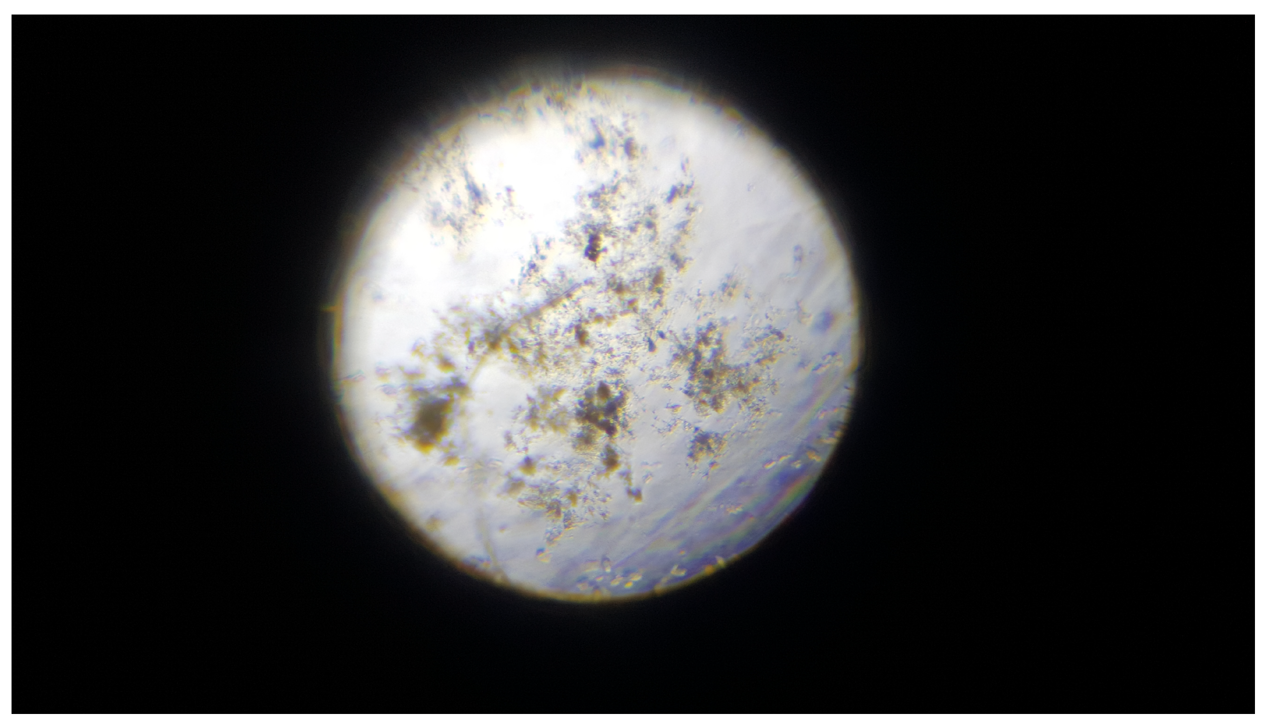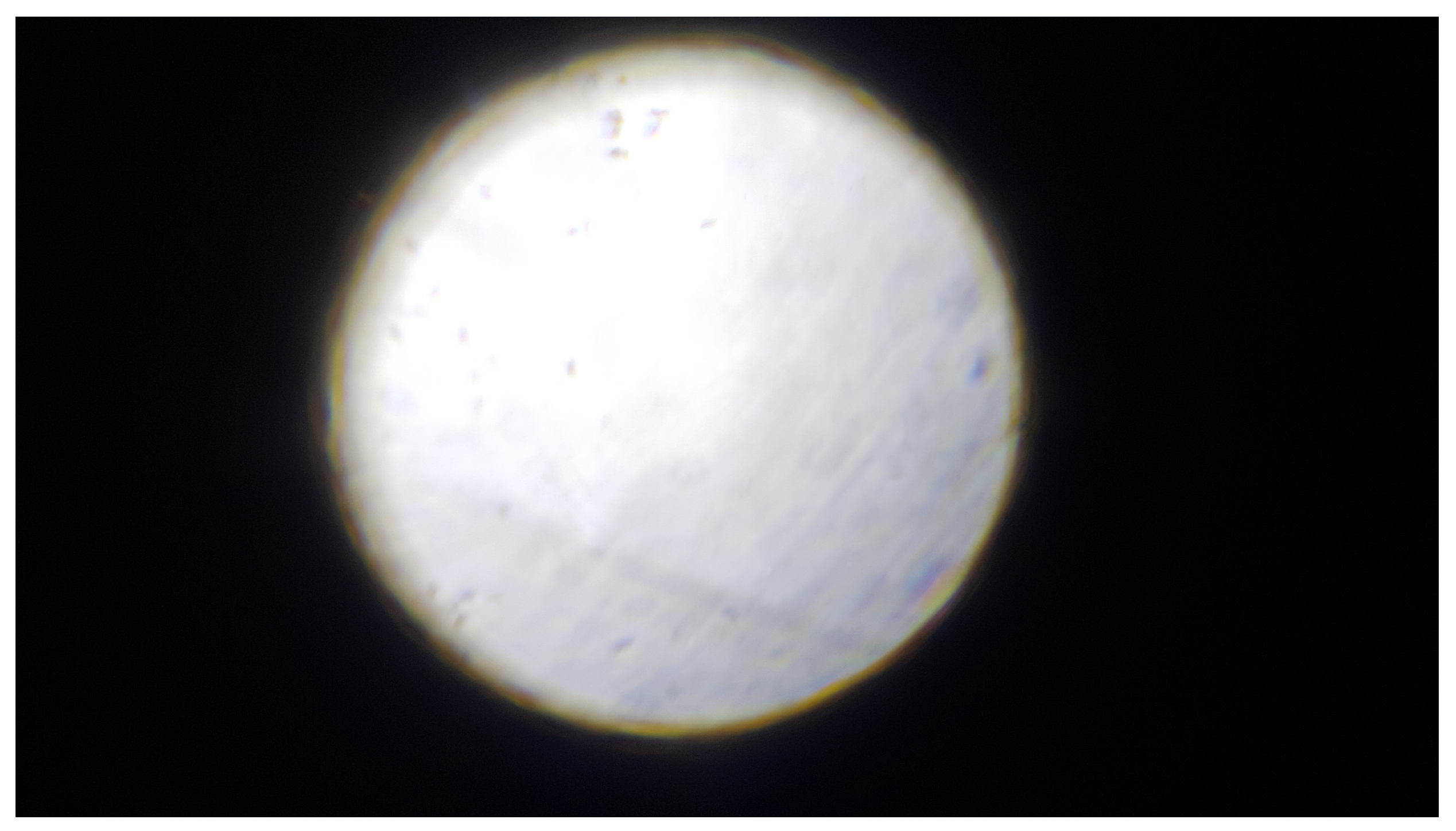Similarities between the data were also described in the study [36]. In addition to these measurements, samples taken from the sea could also be investigated by using microscopes and other sensors. Ohman et al. [37] investigated a study to analyze samples from the sea using optical zoom capability devices. Different types of zooplanktons and mucilage, also known as sea snow, were detected [37]. Totti et al. [38] investigated samples from the sea that were collected from the same locations but at different times: at the time of mucilage bloom and when there was no mucilage. The samples were investigated, and the number and types of plankton were calculated and noted, respectively. In addition, other sensors were used to detect the values of chemicals that were observed in marine mucilage samples by measuring phosphate ($P{O}_4$) and silicate ($Si{O}_4$) values [38]. Giani et al. [39] collected marine mucilage samples from the Northern Adriatic Sea. In the location where the data were collected, some parameters such as temperature, pH, and dissolved oxygen were measured. In addition, the collected data were investigated for their chemical content in the laboratory [39].

Mucilage not only harms the economy by decreasing income from recreation, fishing, and tourism, but it also harms ecology due to the low levels of dissolved oxygen that are observed during mucilage bloom. It affects the food chain of marine fauna [40]. The negative effects of mucilage increase the mortality ratio of different species and are in an extreme manner [40,41,42]. In addition, at the time of mucilage bloom, there is a record of the number of opportunistic species, such as ostracods [43]. Moreover, mucilage also harms the filters of ships; through them, seawater flows into the cooling system of the ship [44].

It is important to solve the aforementioned conditions that occur in order to decrease the volume of mucilage. Moreover, it is also important to prevent marine mucilage on the sea’s surface at the time of mucilage bloom [40]. Collecting mucilage parts on the sea surface helps increase the dissolved oxygen level in the sea [40]. In addition, stopping fishing operations at the time of mucilage bloom can also be useful since fish can eat mucilage [40,45]. Using beneficial bacteria is another way to prevent marine mucilage [46]. For such reasons, it is important to monitor marine mucilage and detect its locations.

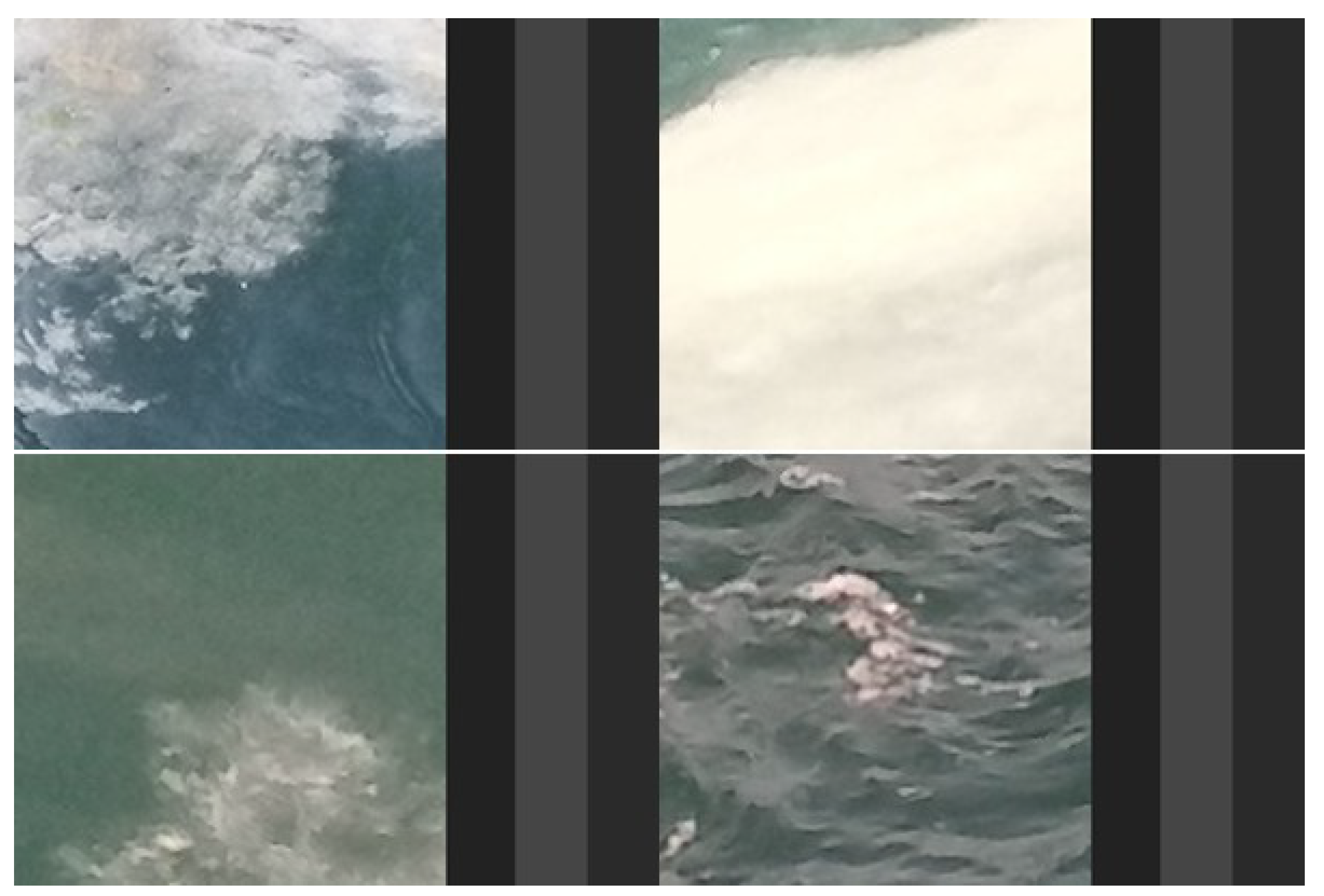
The goal of our study is to improve a system for monitoring marine mucilage on sea surfaces autonomously. There are different ways to monitor marine mucilage, such as using satellite-based or unmanned aerial vehicles (UAV)-based monitoring methods in addition to applying unmanned/manned surface vehicle-based monitoring. However, surface vehicles have the capability to struggle against marine mucilage when using different methods, as explained in the previous paragraph. It is possible to use UAVs to detect mucilage regions and to divert unmanned surface vehicles (USVs) to this region. However, performing both monitoring marine mucilage and preventing it using only one vehicle is more of an economical solution. For this reason, a single USV is accepted as a user of our investigated system. Three different measuring methods are developed in this study for USVs to monitor marine mucilage. First, the USV checks the areas on its route by taking images of the sea’s surfaces. Areas in the images are classified as mucilage candidate areas and non-mucilage areas. If mucilage-candidate areas are identified, the USV is directed to that region. After reaching the mucilage-candidate region, the USV collects data using its sensors, such as a pH meter, dissolved oxygen level sensor, and electrical conductivity sensor. The USV also collects samples from mucilage-candidate areas for analysis either on the USV itself or at the base station by using other sensors or microscopes. This analysis is applied as a useful tool for detecting marine mucilage in suspicious scenarios. Using different types of sensing methods increases the accuracy of detection for the mucilage. In addition, identifying mucilage-candidate regions primarily by using image analysis and directing the USV to those regions also saves time and energy.

2. Materials and Methods

The main goal of this study is to investigate a marine mucilage monitoring system. For this goal, a three-stage marine mucilage monitoring system was used in this study. The stages of the system are described below and shown in Figure 3.

• The sea surface is scanned with a camera operating within a certain radius and photos are taken. The mucilage-candidate areas are determined using image processing, and the USV is directed to mucilage-candidate areas.
• Seawater in the region is measured using the onboard sensors of the surface vehicle.
• The sea is monitored by using microscopes or other sensors via taking samples from the marine mucilage-candidate areas. These samples are evaluated in the laboratory.

The methods mentioned above are explained in the order of their application.

2.1. Monitoring Sea Surface Using Images Taken from Surface Vehicles

Different methods have been proposed for taking pictures of the sea’s surface with the camera placed in the USV and to search for mucilage from the photographs taken by that camera. Before this examination was made, pre-processing steps were necessary if the photographs were to also capture images in addition to the sea’s surface; in other words, the photographs could also include the sky. With these pre-processing steps, the horizon line between the sea and the sky was determined. There are many studies focused on determining the horizon line [47]. Let us briefly explain the method proposed by Sun et al [48] for USVs. In the described method, a horizon line determination method was developed using the line segment detection (LSD) [49] algorithm. The lines in the LSD algorithm include parts of the horizon as well as regions such as islands and ships. In order to prevent this, lines belonging to the horizon line were delineated by making use of the morphological structure and color pattern of the horizon line in the aforementioned study. Then the horizon line was defined by applying rectangle approximation [48].

After the sea’s surface was determined, mucilage areas were then searched for in these images. Different methods have been applied to this search process. One of the methods involves applying an original RGB-based thresholding method developed by the authors of this study. Apart from this, CNN, kNN, SVM and feed-forward neural network (FFNN) methods were also applied. The methods applied and the results achieved are explained in the subsections of this paper.

The data used to develop the described methods were drawn from vessels navigating the Sea of Marmara. Figure 4, Figure 5 and Figure 6 are some examples of the photographs used. Some of the photographs in this data set contain marine mucilage, and some do not.

2.1.1. RGB-Based Marine Mucilage Monitoring Method

Images of sea surfaces with and without mucilage were examined. These images were taken from different regions and at different periods with respect to daylight intensity. Mucilage and non-mucilage samples were randomly taken samples from the obtained photographs. However, as observed in Figure 4, it is quite possible that the wave foam and mucilage formed as a result of the movement of the surface vehicles in the same image. It is important to distinguish between the wave foam created by the USVs (that the system intends to use) and the wave foam created by other surface vehicles.

Sunlight has an important effect on photographs taken from the sea surface. To avoid this effect, normalization was applied to the images of sea surfaces. After normalization, the images were transformed into binary images. In binary images, white pixels indicate mucilage-candidate areas. The results were obtained when this developed method was applied to Figure 4, Figure 5 and Figure 6, and the results are shown in Figure 7. The developed RGB-based method is detailed in Appendix A.

2.1.2. Resnet-50 Based Marine Mucilage Monitoring Method

Artificial intelligence methods are widely used for the classification and detection of objects in image processing [50]. The accuracy level of convolutional neural networks (CNN), which is one of the artificial intelligence methods, is accepted as satisfactory in the field of image analysis [50]. CNN-based object classifying applications have a wide range of applications, such as face recognition, object detection on motorways, or vessel detection in maritime environments [50,51,52]. There are different layers inside CNNs, which include the input layer, convolution layer, and pooling layer, which is typically activated by the rectifier linear unit layer and fully connected layer [50].

Many neural network systems are focused on deeper learning. However, the deeper the learning, the more successful results do not necessarily follow. Resnet, the name of which comes from the unification of residual and network, illustrates this phenomenon. The main goal of Resnet is to produce more permanent results in image applications, such as object classification [50]. The Resnet-50 method, which was investigated by He et al. [53], was applied in this study to detect non-mucilage and mucilage-candidate regions. For this purpose, the images of the sea surfaces were divided into small regions in 150 × 150 pixels. These regions are presented to the previously trained Resnet-50 network. The regions determined as mucilage by the network as a result of classification are accepted as mucilage-candidate regions. The training data were randomly selected from the regions with and without mucilage, and the data set comprising 4100 mucilage and 4100 mucilage-free photographs was tested. One-third of these photographs were randomly selected as test data, and the remaining photographs were used as training data. The results are described in the next chapter.

2.1.3. kNN Based Marine Mucilage Monitoring Method

The k-nearest neighbor algorithm is a pattern classification method, and is widely used as a classifier [54]. This algorithm measures the distance between unlabeled observations and the sample data. Using the result of this measurement determines the class to which the observation’s results belong. The simplicity, high success rate, and well-known nature of the kNN algorithm make it a popular algorithm. The number of parameters used in the kNN algorithm can be determined according to the size of the preferred training data [55]. The kNN algorithm can use different distance measurement methods including Euclidean and Manhattan distances [56]. Prasath et al. suggested that both methods work with similar accuracies [55]. The basic working algorithm of the kNN method is as follows. According to the distance metric chosen, the training data located within the neighborhood of the determined k value of the sample (test sample) to be classified are verified. Depending on the class that has more training samples in this k neighborhood, the relevant test sample is determined as belonging to that class [55,57]. The kNN algorithm has a huge usage area. An example of this is the classification of the different color space information data with respect to polluted and clean areas on the beaches using the kNN algorithm [17].

In this study, luminance-based YCbCr, perceptually uniform (CIE-Lab), and hue-based (HSV) color spaces are also used in addition to the RGB color space to increase the accuracy of classification. A data set was created from 15 × 15 visuals of regions with and without mucilage. R, G, B, Y, Cb, Cr, H, S, V, CIE-L, CIE-A, and CIE-B values of 225 pixels in these 15 × 15 images were averaged within themselves. A sequence of values calculated in this manner represents an example. A number of 1125 samples with mucilage and 1125 samples without mucilage were randomly selected. Care was taken to include both the sea surface alone and the sea surface samples containing wave foam in non-mucilage samples. In addition, samples taken under different daylight conditions were included in both training data groups. These examples are presented to the kNN algorithm in two ways. In the first method, predetermined data involving 1800 instances were used as training data, 450 ones of data were used as test data, and the result was obtained. In the second method, 10% of the training data were randomly allocated as test data, and all data were used as both training and test data by subjecting them to 10-fold cross-validation. For both methods, the k-value of the kNN algorithm was chosen as 5. The results are provided in the next chapter.

2.1.4. SVM Based Marine Mucilage Monitoring Method

The support vector machine is a classification method that aims to distinguish data into two classes. The aim is to maximize the distance between the classes in their separation from one another. An abundance of distinctive planes can be created in the distribution of data into the two classes. Here, the plane that maximizes the distance between the most remote elements of the separated classes is chosen as the distinctive plane [58,59]. Similar to the kNN application, the samples are presented to the SVM algorithm using the two methods described above. The results are provided in the next chapter.

2.1.5. Feed Forward Neural Network Based Marine Mucilage Monitoring Method

A feed-forward neural network (FFNN) is a commonly used artificial neural system that comprises multi layers. The first layer is an entry point of inputs into the system [60]. In feed-forward neural networks, the cells are arranged in layers, and the outputs of cells in one layer are input to the next layer via weights. The network output is determined by processing information in the middle and output layesr. With this structure, feed-forward networks perform a non-linear static function. It has been shown that a 3-layer FFNN can approximate any continuous function with the desired accuracy, provided that there are a sufficient number of cells in its middle layer [61]. A 3-layer FFNN consists of an input layer, an output layer, and a hidden layer [61]. An example of this type of FFNN is given in Figure 8. In this study, a 3-layer FFNN was used. The input layer received 12 different data instances, while the output layer projected the incoming data into two separate classes: mucilage-candidate and non-mucilage.

2.1.6. Comparison with Other Data Set

In the literature, as observed thus far, we have not discovered data sets used in publications targeting the processing of mucilage images taken from marine vessels. For this reason, and as a focus of this study, we examined studies focused on processing images taken from marine vessels and investigated the data set used in those studies.

For the classification of sea ice species, the work studied by Dowden et al. [33] was chosen as a comparative case study. In that study, the data set was created with screenshots taken from an icebreaker ship operating in Antarctica and from a video uploaded on YouTube at youtu.be/BNZu1uxNvlo [33]. In a related study, images in this data set were subjected to multiple classification operations, and they were classified as the ocean, first-year ice, gray ice, new ice, etc., and divided into classes. From the aforementioned YouTube video, 150 × 150 pixel images were created in 2 different groups, 320 of which contained only first-year ice and 320 images containing parts of the ocean, gray-ice, or new ice. In both groups, 80% of the data set was used for training, and 20% of the data set was used for testing. Comparing that study with ours will not yield meaningful results due to the different methods used, the different number of classes, etc. The purpose of using this dataset was to demonstrate that only the classification proposed by us is acceptable. The PSPNet101 method used in the aforementioned study is a method developed from the Resnet method [33]. In this respect, the results of the Resnet-50 method used in our study and the average results of the PSPNet101 method used in the aforementioned study are provided together in the next section.

In addition, the method suggested by Tian et al. [27] is also discussed. In their method, sea ice was searched in sea surface images using the SVM method, similar to other methods [27]. On the above-mentioned data set, pixels containing sea ice were searched for using the SVM method. The results are provided in the next section. Similarly to the previous method, it is meaningless to compare directly the results found by us in this method with the results in the mentioned work. The purpose of performing the application and providing the results in this data set is to show that the procedure is in accordance with studies in the literature and that the success rate is within acceptable limits.

The results are provided in the next section.

2.2. Marine Mucilage Monitoring Using On-Board Sensors

In 2021, samples were taken from the Marmara Sea, Istanbul, Anatolian Side, during the mucilage bloom period and during the normal period. The samples taken were measured with pH meters and electrical conductivity sensors. These measurement results were compared with the study van Eenennaam et al. [34]. Two artificial samples were also created to compare with the measurements made. In the first artificial sample, a natural acidic substance was added to standard seawater until it brought the pH level of this seawater to that of mucilage seawater. In the other artificial sample, a basic substance was added to the standard sample. With the basic substance added, the electrical conductivity of this sample was ensured to be equal to the mucilage sample. Measurements were made with the 86031 AZ IP67 model instrument of AZ Instrument Corp.

The samples used in the measurements are summarized in

Table 1. Samples used in the measurements via onboard sensors.

Sample Number	Sample Type
Sample-1	Istanbul Anatolian Side Standard (Mucilage-Free) Sea Water (IASSSW)
Sample-2	Istanbul Anatolian Side Mucilage Sea Water
Sample-3	Sea Water (IASSSW) + Acidic Waste (Soluble in Sea Water)
Sample-4	Sea Water (IASSSW) + Basic Waste (Soluble in Sea Water)

.

2.3. Marine Mucilage Monitoring Using Microscopes

In this study, it was predicted that a USV tasked with mucilage monitoring had the ability to take samples in addition to performing image processing and possessing measurement capabilities using onboard sensors. The samples discussed here can be measured with an in-vehicle microscope that is capable of autonomous focusing, or the samples can be measured in the laboratory to which they are taken. There are studies in the literature regarding this topic. For example, Ohman et al. determined the plankton species and mucilage by using a sampling device and FLIR camera attached to the USV [37].

In this study, a very low-cost JWIN JM-452M model microscope with 100×, 400×, and 1200× optical zoom features was used only in the 100x mode. A lower specification microscope was preferred as the goal was only to determine if mucilage was present. The data set used in this study consists of 35 mucilage and 35 non-mucilage microscope images. Some sample images are provided in Figure 9 and in Figure 10. The aforementioned data were processed using two different methods, and a distinction between mucilage-candidate sea water and non-mucilage sea water was attempted. The first of the methods was based on RGB-based thresholding. As for the second method, the CNN-based Resnet-50 method was used.

2.3.1. RGB Thresholding Based Marine Mucilage Monitoring Method Using Microscope

In this study, a method was proposed for the determination of mucilage-candidate and non-mucilage samples by using the grayscale pixel values of the pixels. When performing this step, the arithmetic means and mean square error methods were used, and thresholding was conducted.

First of all, the related photos were converted into grayscale. Then, the pixels surrounding the image from the lens in the photograph and the border regions of the lens with these black surrounding pixels were identified and separated. The remaining pixels were then averaged. The average is the first parameter. As for the second parameter, the value was obtained by dividing the mean by the value of the relevant pixel. For each pixel in this picture, this value was calculated by the mean square error method. The mean grayscale and the mean square error values were evaluated together to decide whether the picture belonged to the mucilage-candidate or non-mucilage category. The pseudo-code of this account is provided in Figure 11. The results are described in the next section.

2.3.2. Resnet-50 Based Marine Mucilage Monitoring Method Using Microscope

The Resnet-50 method, which is a CNN-based method, was explained in Section 2.1.2. Here, 24 data instances comprising both types (mucilage-candidate/non-mucilage) were reserved for training and 11 for testing purposes. The test’s results are explained in the next section.

2.4. Marine Mucilage Monitoring via Fusion of Image Processing and Onboard Sensors

Data fusion is created by bringing together different sources and is applied in many areas where the information flow from different sources is provided. Birogul et al. explained data fusion as a method of combining data flowing from many different sensors in order to conduct better evaluations than using data received from only one sensor [62]. Sensor fusion is also a subfield of data fusion. The use of different types of sensors observing the same event and the evaluation of the information received from different sensors together is called sensor fusion [63]. The data collected from different sensors are evaluated together with various static and dynamic methods. Autonomous vehicle applications can be given as an example of sensor fusion applications [64]. In the cases where the antenna used is quite large, it becomes difficult for humans to observe these antennas and to monitor discrete and instant information, which increases the need for sensor fusion [65]. In addition, obtaining better classification results and providing a more robust approach are among the reasons why sensor fusion is the preferred method [66].

In the fusion scenario of this study, a USV that is on patrol both takes a picture of the area it travels through during its route and receives onboard sensor data related to this area; the data are subjected to sensor fusion processes. For this goal, RGB photos with the size of 150 × 150 pixels and data from onboard sensors were fused and given to the Resnet-50 network, increasing the success rate. While doing this, the data received from the dissolved oxygen sensor was multiplied by 10 (in mg/L), then the calculated value was rounded to an integer and the first parameter value was found. Similarly, the second parameter value was calculated by multiplying by 10 the data received from the pH sensor. Finally, the data obtained from the electrical conductivity sensor were rounded to an integer, and the third parameter was obtained. All three parameters are converted to images with a size of 150 × 25 pixels separately. The R, G, and B parameters of all pixels of these images are assigned the same value. Images derived from these three parameters were combined with 150 × 150 pixel images. Examples of the combined pictures without mucilage are provided in Figure 12. Moreover, examples of the combined pictures with mucilage are provided in Figure 13.

A new data set of 8200 photographs were created by adding sensor data to 4100 mucilage and 4100 mucilage-free photographs. Of this data set, 66% of photographs were allocated as training data and 34% of photographs as test data and given to the Resnet-50 network. The results of these data are provided in the next chapter.

2.5. Marine Mucilage Monitoring Using Other Methods

With USVs, marine mucilage monitoring can be performed with different methods than those mentioned above. Although the three-step method described in this study provides sufficient accuracy for marine mucilage monitoring, in our opinion, some alternative methods are also explained here.

2.5.1. Marine Mucilage Monitoring Method Using Turbidity Sensor

Turbidity data can also be used to measure mucilage. There is a study showing that turbidity increases during mucilage bloom [2]. The turbidity levels of standard seawater were compared with the sample taken during the mucilage bloom period in the Marmara Sea. In the comparison, it was observed that mucilage seawater had 3% more turbidity.

The turbidity sensor used in this study is the DF Robot SKU SEN 0189 model turbidity sensor [67]. This sensor has two plastic waterproof protrusions. These two protrusions form a channel between them that allows water to flow. One of the protrusions has an LED, and the other has a photo-transistor. Depending on the turbidity of the water, the light intensity falling on the photo-transistor changes, which affects the output voltage. The output voltage is read in the analog-to-digital converter, and the turbidity difference between the samples is thus obtained.

2.5.2. Marine Mucilage Monitoring Method Using Phosphate Measuring

It is known that the increase in nutrient-loaded wastes released into seawaters triggers ecological events that cause mucilage [2]. For this reason, we expect high levels of substances considered as nutrient load in the mucilage water. This can also be observed in the literature [38]. Mucilage and non-mucilage seawater samples collected within the scope of this study were measured in terms of different components. We performed comparisons with respect to these components. Phosphate was mostly observed in different amounts in both the mucilage and non-mucilage samples, and the amount of phosphate in the mucilage sample was much higher. Phosphate measurements comprise one of the methods that can be used to determine mucilage-candidate regions, and this is consistent with other studies in the literature.

3. Results

3.1. Results for Marine Mucilage Monitoring with Sea Surface Images

3.1.1. Results for Resnet-50 Method on Sea Surface Images

First, the data were divided randomly into 512 training data and 128 test data instances. The number of samples with and without mucilage was equal in both groups. For this experiment, precision (P), recall (R), and F-Score (F) values were calculated. The formulas used to calculate these values are provided below [17]:

$$P(\%)=\frac{TP}{TP+FP}\times 100$$

(1)

$$R(\%)=\frac{TP}{TP+FN}\times 100$$

(2)

$$F(\%)=2\frac{PR}{P+R}\times 100$$

(3)

The results are provided in

Table 2. Results of Resnet-50 algorithm for 512 training samples and 128 test samples.

Algorithm	TP	FN	FP	P(%)	R(%)	F(%)
Resnet-50	56	8	2	96.55	87.50	91.80

.

3.1.2. Results of kNN, SVM and FFNN Algorithms

Classification using kNN, SVM, and FFNN algorithms was tested in two different methods. First, the data were divided into 1800 samples of training data and 450 samples of test data. The number of samples with and without mucilage was equal in both groups. After true-positive, true-negative, false-positive, and false-negative values were found, precision, recall, and F-Score values were calculated. The results are provided in

Table 3. Results of kNN, SVM and FFNN algorithms for 1800 training samples and 450 test samples.

Classifier	TP	FN	FP	P(%)	R(%)	F(%)
kNN	214	11	17	92.64	95.11	93.86
SVM	213	12	26	89.12	94.67	91.81
FFNN	214	11	13	94.27	95.11	94.69

.

As described in Section 2.3–Section 2.5, 10-fold cross-validation was also performed with kNN, SVM, and FFNN algorithms. The result of each cross-validation was averaged. These results are provided in

Table 4. Mean results of kNN, SVM, and FFNN algorithms for 2250 samples in a 10-fold cross-validation scheme.

Classifier	TP	FN	FP	P(%)	R(%)	F(%)
kNN	106.9	5.6	5.2	95.36	95.02	95.19
SVM	106.2	6.3	4.1	96.28	94.22	95.24
FFNN	109.4	3.1	5.2	95.46	97.24	96.34

.

3.1.3. Results of Using Methods in Other Data Set

First of all, the results of the classification study on the sea-ice data were obtained from the YouTube video (provided as the dataset source by Dowden et al. [33]). Since the Resnet-based PSPNet101 method was used in the aforementioned study, those results are also shared in

Table 5. Results of sea-ice classification explained Section 2.1.6.

Sample Number	Sample Type
Classifier	TP	FN	FP	P(%)	R(%)	F(%)	FPR	FNR	Accuracy
SVM	209	10	16	92.89	95.43	94.14	0.0692	0.0457	0.9422
Resnet-50	63	4	1	98.43	94.03	96.18	0.016	0.0597	0.9609
PSPNet101 of [33]	-	-	-	-	-	-	0.005	0.077	-
SVM Result of [27]	-	-	-	-	-	-	-	-	0.8

. The metrics used are provided below:

$$Accuracy=\frac{TP+TN}{TP+FP+TN+FN}$$

(4)

$$FPRate\left(FPR\right)=\frac{FP}{TN+FP}$$

(5)

$$FNrate\left(FNR\right)=\frac{FN}{TN+FP}$$

(6)

At the same time, the SVM method was used in the sea-ice study conducted by Tian et al. [27]. In Table 5, the results obtained with the kNN and SVM method for the sea-ice classification are shared. As explained in Section 2.1.6, it is not meaningful to directly compare the results here with those in related publications. The aim is only to explain that the applied classification method is also used in studies that classify differences on sea surfaces and in the images taken with surface vehicles and to state that the results that we found were within acceptable limits.

3.2. Results of On-Board Sensors

The sensor results specified in Section 2.3 are classified and explained by sensor type. In addition, comparisons of these results with those in the literature are provided in the next chapter.

Dissolved oxygen level values of samples are given in

Table 6. Dissolved oxygen level values of samples.

Sample Number	Dissolved Oxygen Level (mg/L)
Sample-1	5.2
Sample-2	3.6
Sample-3	5.3
Sample-4	4

.

The pH measurement results of samples are provided in

Table 7. pH measurement results of samples.

Sample Number	pH Level
Sample-1	8.25
Sample-2	7.03
Sample-3	7.04
Sample-4	10.2

.

The electrical conductivity measurements of samples are provided in

Table 8. Electrical conductivity measurement results of samples.

Sample Number	Electrical Conductivity (mS)
Sample-1	36.4
Sample-2	44
Sample-3	37
Sample-4	43

.

3.3. Results for Marine Mucilage Monitoring with Microscope Image Data

The results obtained when the RGB-based method and the Resnet-50 method were applied to 35 with marine mucilage and 35 non-mucilage photographs are provided in

Table 9. Results of classification of microscope photographs for marine mucilage.

Classifier	TP	FN	FP	P(%)	R(%)	F(%)
RGB-Based	34	1	1	97.14	97.14	97.14
Resnet-50 Based	10	1	1	90.9	90.9	90.9

. In the Resnet-50 method, 24 images from both groups were used for training, and 11 photographs were used for testing purposes.

Due to the scarcity of data subject to classification, the success of the Resnet-50 method was considered low, and we predict that if the data set is enlarged, the success rate will be higher, similar to the work conducted in this study, for which its results are shown in Table 2.

3.4. Results of Marine Mucilage Monitoring via Fusion of Image Processing and Onboard Sensors

In total, 4100 with mucilage and 4100 without mucilage images, which contain images and information about three different onboard sensors, were inputted into the Resnet-50 Network. Of these images, 66% were used for training, and 34% were used for testing purposes. The results produced by the network are provided in

Table 10. Results of Resnet-50 algorithm for 5412 training samples and 2788 test Samples for fusion images.

Classifier	TP	FN	FP	P(%)	R(%)	F(%)
Resnet-50	1176	218	34	97.87	98.85	98.34

.

4. Discussion

The application of unmanned surface vehicles is becoming increasingly common. In this study, it was predicted that unmanned surface vehicles could be used to monitor marine mucilage, which has become a common problem in many countries in the Mediterranean Basin, especially in Turkey. The support of a project for the use of UAV and USV together in the struggle against marine mucilage by an institution of the Turkish State also supports this previous assertion [68]. Unmanned surface vehicles can collect marine mucilage from the sea surface when mucilage blooms, in addition to monitoring mucilage. A three-stage mucilage determination system was envisaged to fulfill this task.

In the first step, the areas suspected of comprising mucilage were determined by using image processing. In this study, the image-based mucilage detection application was implemented using five different methods. All applied methods have been sufficiently successful and are preferred. The highest success rate was obtained by the FFNN method. Since the FFNN method has the highest success rate, using the FFNN method in the first stage (image processing) is strongly recommended if a computer with sufficient processing capability is available on the USV. In the second step, parameters such as pH, electrical conductivity, and dissolved oxygen level were measured in areas suspected of containing mucilage. In the literature (for example, in [34,40,42]), it has been stated that mucilage causes a decrease in oxygen levels in the seawater. Therefore, these measurements, provided in Table 6, are in line with studies in the literature. In addition, in the literature (for example, in [34]), it has been stated that mucilage causes a decrease in the pH level in seawater. Therefore, these measurements provided in Table 7 are in line with the studies in the literature. It has been explained in the literature that similar salinity levels were observed in the two different seas of the Mediterranean Sea during the mucilage bloom period: the Adriatic Sea and the Ligurian Sea [36]. Therefore, it can be expected that the salinity level will change during the mucilage period, and accordingly, electrical conductivity will change. In this respect, it can be said that the information provided in Table 8 is in accordance with the literature. The use of three different sensors allows the separation of with-mucilage seawater not only from non-mucilage (standard) seawater but also from seawater contaminated with the heavily acidic or heavily basic matter. This situation is shown in Table 6, Table 7 and Table 8. Sample 3 in these tables represents an intensely acidic pollutant, and Sample-4 represents an intensely basic pollutant which is described in Section 2.2. As a third step, samples were taken from the area suspected of containing mucilage, and the samples were examined under a microscope in the laboratory. Two different methods were used in this study. The success rates of the proposed methods are at an acceptable level. However, using the RGB-based method is recommended since the microscope examination is performed under controlled conditions.

In addition, two studies on the search for sea ice on the sea’s surface were also discussed for comparison purposes. In the comparison, it is observed that the methods applied here can also be used in alternative monitoring applications on the sea’s surface. There are studies that detected sea ice on the sea’s surface for manned or unmanned surface vehicles or observed pollution such as oil spills. For marine mucilage, studies have been conducted to determine marine mucilage with images taken from satellite or manned/unmanned aerial vehicles. In this study, unlike previous studies, we aimed to monitor marine mucilage areas for unmanned surface vehicles. Our results were compared with other studies in Section 3.1.3 that focused on classification of the sea’s surface. We show that our results are within the acceptable range.

In this study, it was assumed that image acquisition, onboard sensor usage, and sample-taking processes were carried out in appropriate meteorological conditions. Under adverse meteorological conditions, it may be necessary to establish a number of supporting mechanisms so that the specified measurements can be made with acceptable accuracy. This issue will be addressed by the authors in future studies. Another possible scenario, which takes pictures and collects onboard sensor data on a determined patrol route, is considered, and in this scenario, the images taken from the camera are combined with three different onboard sensor data and entered into the Resnet-50 Network. The results produced by the network have a very high success rate. Therefore, it is possible to consider that this method is quite useful and successful when the USV is required to follow a certain route continuously in its search for mucilage.

The authors of this study intend to develop an unmanned surface vehicle for mucilage monitoring and collection or intend to participate in studies conducted for this purpose in the near future. We also aim to design the underwater scanning features with mucilage in mind in addition to the surface mission requirements.

References

1. Yagci, A.L.; Colkesen, I.; Kavzoglu, T.; Sefercik, U.G. Daily monitoring of marine mucilage using the MODIS products: A case study of 2021 mucilage bloom in the Sea of Marmara, Turkey. Environ. Monit. Assess. 2022, 194, 1–20. [Google Scholar] [CrossRef] [PubMed]
2. Komuscu, A.U.; Aksoy, M.; Dogan, O.H. An Analysis of Meteorological Conditions in Relation to Occurrence of the Mucilage Outbreaks in Sea of Marmara, March-June 2021. Int. J. Environ. Geoinform. 2022, 9, 126–145. [Google Scholar] [CrossRef]
3. Rasuly, A.; Naghdifar, R.; Rasoli, M. Monitoring of Caspian Sea coastline changes using object-oriented techniques. In Proceedings of the International Society for Environmental Information Sciences 2010 Annual Conference, Beijing, China, 27–29 August 2010; pp. 416–426. [Google Scholar]
4. Bondur, V.G. Complex satellite monitoring of coastal water areas. In Proceedings of the 31st International Symposium on Remote Sensing of Environment, St. Petersburg, Russia, 20–24 May 2005. [Google Scholar]
5. Messager, C.; La, T.V.; Sahl, R.; Dupont, P.; Prothon, E.; Honnorat, M. Use of SAR Imagery and Artificial Intelligence for a Multi-Components Ocean Monitoring. In Proceedings of the IGARSS 2020 IEEE International Geoscience and Remote Sensing Symposium, Waikoloa, HI, USA, 26 September–2 October 2020; pp. 3817–3820. [Google Scholar]
6. Ferreira, A.; Brito, A.C.; Mendes, C.R.B.; Brotas, V.; Costa, R.R.; Guerreiro, C.V.; Sá, C.; Jackson, T. OC4-SO: A New Chlorophyll-a Algorithm for the Western Antarctic Peninsula Using Multi-Sensor Satellite Data. Remote Sens. 2022, 14, 1052. [Google Scholar] [CrossRef]
7. Khan, A.A.; Jamil, A.; Hussain, D.; Taj, M.; Jabeen, G.; Guerreiro, C.V.; Malik, M.K. Machine-Learning Algorithms for Mapping Debris-Covered Glaciers: The Hunza Basin Case Study. IEEE Access 2020, 84, 12725–12734. [Google Scholar] [CrossRef]
8. Shen, X.; Zhang, J.; Zhang, X.; Meng, J.; Ke, C. Sea ice classification using Cryosat-2 altimeter data by optimal classifier–feature assembly. IEEE Geosci. Remote Sens. Lett. 2017, 140, 1948–1952. [Google Scholar] [CrossRef]
9. Gokaraju, B.; Durbha, S.S.; King, R.L.; Younan, N.H. Sensor web and data mining approaches for Harmful algal bloom detection and monitoring in the Gulf of Mexico region. In Proceedings of the2009 IEEE International Geoscience and Remote Sensing Symposium, Cape Town, South Africa, 12–17 July 2009; Volume III, pp. 789–792. [Google Scholar]
10. Hereher, M.E. Climate Change during the Third Millennium—The Gulf Cooperation Council Countries. Sustainability 2022, 14, 14181. [Google Scholar] [CrossRef]
11. Kavzoğlu, T.; Tonbul, H.; Çölkesen, İ; Sefercik, U.G. The Use of Object-Based Image Analysis for Monitoring 2021 Marine Mucilage Bloom in the Sea of Marmara. Int. J. Environ. Geoinform. 2021, 8, 529–536. [Google Scholar] [CrossRef]
12. Cavalli, R.M. Retrieval of Sea Surface Temperature from MODIS Data in Coastal Waters. Sustainability 2017, 9, 2032. [Google Scholar] [CrossRef]
13. Acar, U.; Yilmaz, O.S.; Celen, M.; Ates, A.M.; Gulgen, F.; Sanli, F.B. Determination of mucilage in the Sea of Marmara using remote sensing techniques with google earth engine. Int. J. Environ. Geoinform. 2021, 8, 423–434. [Google Scholar] [CrossRef]
14. Tassan, S. An algorithm for the detection of the White-Tide (“mucilage”) phenomenon in the Adriatic Sea using AVHRR data. Remote Sens. Environ. 1993, 45, 29–42. [Google Scholar] [CrossRef]
15. Pinto, L.; Andriolo, U.; Gonçalves, G. Detecting stranded macro-litter categories on drone orthophoto by a multi-class Neural Network. Mar. Pollut. Bull. 2021, 169, 112594. [Google Scholar] [CrossRef] [PubMed]
16. Gonçalves, G.; Andriolo, U.; Pinto, L.; Duarte, D. Quantifying Mapping marine litter with Unmanned Aerial Systems: A showcase comparison among manual image screening and machine learning techniques. Mar. Pollut. Bull. 2020, 155, 111158. [Google Scholar] [CrossRef] [PubMed]
17. Gonçalves, G.; Andriolo, U.; Gonçalves, L.; Sobral, P.; Bessa, F. Quantifying Marine Macro Litter Abundance on a Sandy Beach Using Unmanned Aerial Systems and Object-Oriented Machine Learning Methods. Remote Sens. 2020, 12, 2599. [Google Scholar] [CrossRef]
18. Fallati, L.; Polidori, A.; Salvatore, C.; Saponari, L.; Savini, A.; Galli, P. Anthropogenic Marine Debris assessment with Unmanned Aerial Vehicle imagery and deep learning: A case study along the beaches of the Republic of Maldives. Sci. Total Environ. 2019, 693, 133581. [Google Scholar] [CrossRef] [PubMed]
19. Kim, D.H.; Seo, J.N.; Yoon, W.D.; Suh, Y.S. Estimating the economic damage caused by jellyfish to fisheries in Korea. Fish. Sci. 2012, 78, 1147–1152. [Google Scholar] [CrossRef]
20. Kim, H.; Koo, J.; Kim, D.; Jung, S.; Shin, J.U.; Lee, S.; Myung, H. Image-based monitoring of jellyfish using deep learning architecture. IEEE Sens. J. 2016, 16, 2215–2216. [Google Scholar] [CrossRef]
21. Narmilan, A.; Gonzalez, F.; Salgadoe, A.S.A.; Kumarasiri, U.W.L.M.; Weerasinghe, H.A.S.; Kulasekara, B.R. Predicting Canopy Chlorophyll Content in Sugarcane Crops Using Machine Learning Algorithms and Spectral Vegetation Indices Derived from UAV Multispectral Imagery. Remote Sens. 2022, 14, 1140. [Google Scholar] [CrossRef]
22. Gonçalves, D.; Gonçalves, G.; Pérez-Alvávez, J.A.; Andriolo, U. On the 3D Reconstruction of Coastal Structures by Unmanned Aerial Systems with Onboard Global Navigation Satellite System and Real-Time Kinematics and Terrestrial Laser Scanning. Remote Sens. 2022, 14, 1485. [Google Scholar] [CrossRef]
23. Li, X.; Shang, S.; Lee, Z.; Lin, G.; Zhang, Y.; Wu, J.; Kang, Z.; Liu, X.; Yin, C.; Gao, Y. Detection and Biomass Estimation of Phaeocystis globosa Blooms off Southern China From UAV-Based Hyperspectral Measurements. IEEE Trans. Geosci. Remote Sens. 2021, 60, 1–13. [Google Scholar] [CrossRef]
24. Zambianchi, E.; Calvitti, C.; Pcecamore, F.D.; Ferulano, E.; Lanciano, P. The mucilage phenomenon inthe northern Adriatic Sea, summer 1989: A study carried outwith remote sensing techniques. In Proceedings of the International Conference Marine Coastal Eutrophication, Bologna, Italy, 21–24 March 1990; pp. 581–598. [Google Scholar]
25. Verfuss, U.K.; Aniceto, A.S.; Harris, D.V.; Gillespie, D.; Fielding, S.; Jiménez, G.; Johnston, P.; Sinclair, R.R.; Sivertsen, A.; Solbo, A.S.; et al. TA review of unmanned vehicles for the detection and monitoring of marine fauna. Mar. Pollut. Bull. 2019, 140, 17–29. [Google Scholar] [CrossRef]
26. Marini, S.; Gjeci, N.; Govindaraj, S.; But, A.; Sportich, B.; Ottaviani, E.; Márquez, F.P.G.; Bernalte Sanchez, P.J.; Pedersen, J.; Clausen, C.V.; et al. ENDURUNS: An Integrated and Flexible Approach for Seabed Survey Through Autonomous Mobile Vehicles. J. Mar. Sci. Eng. 2020, 8, 633. [Google Scholar] [CrossRef]
27. Tian, K.; Liu, Z.; Li, L.; Zhou, N.; Zhao, Y. The Multi-Parameter Monitoring Method of Sea Ice Based on Image Processing Technique. In Proceedings of the 2021 IEEE 11th Annual International Conference on CYBER Technology in Automation, Jiaxing, China, 27–31 July 2021; pp. 510–513. [Google Scholar]
28. Cao, H.; Guo, Z.; Wang, S.; Cheng, H.; Zhan, C. Intelligent Wide-Area Water Quality Monitoring and Analysis System Exploiting Unmanned Surface Vehicles and Ensemble Learning. Water 2020, 12, 681. [Google Scholar] [CrossRef]
29. Dąbrowski, P.S.; Specht, C.; Specht, M.; Burdziakowski, P.; Makar, A.; Lewicka, O. Integration of multi-source geospatial data from GNSS receivers, terrestrial laser scanners, and unmanned aerial vehicles. Can. J. Remote Sens. 2021, 47, 621–634. [Google Scholar] [CrossRef]
30. Specht, M.; Stateczny, A.; Specht, C.; Widźgowski, S.; Lewicka, O.; Wiśniewska, M. Concept of an Innovative Autonomous Unmanned System for Bathymetric Monitoring of Shallow Waterbodies (INNOBAT System). Energies 2021, 14, 5370. [Google Scholar] [CrossRef]
31. Papachristopoulou, I.; Filippides, A.; Fakiris, E.; Papatheodorou, G. Vessel-based photographic assessment of beach litter in remote coasts. A wide scale application in Saronikos Gulf, Greece. Mar. Pollut. Bull. 2020, 150, 110684. [Google Scholar] [CrossRef]
32. Wang, J.; Ren, F.; Li, Z.; Liu, Z.; Zheng, X.; Yang, Y. Unmanned surface vessel for monitoring and recovering of spilled oil on water. In Proceedings of the OCEANS 2016, Shanghai, China, 10–13 April 2016. [Google Scholar]
33. Dowden, B.; De Silva, O.; Huang, W.; Oldford, D. Sea ice classification via deep neural network semantic segmentation. IEEE Sensors J. 2020, 21, 11879–11888. [Google Scholar] [CrossRef]
34. Van Eenennaam, J.S.; Rahsepar, S.; Radović, J.R.; Oldenburg, T.B.; Wonink, J.; Langenhoff, A.A.M.; Murk, A.J.; Foekema, E.M. Marine snow increases the adverse effects of oil on benthic invertebrates. Mar. Pollut. Bull. 2018, 126, 339–348. [Google Scholar] [CrossRef] [PubMed]
35. Sieber, A.; Cocco, M.; Markert, J.; Wagner, M.F.; Bedini, R.; Dario, P. ZigBee based buoy network platform for environmental monitoring and preservation: Temperature profiling for better understanding of Mucilage massive blooming. In Proceedings of the International Workshop on Intelligent Solutions in Embedded Systems, Regensburg, Germany, 10–11 July 2008. [Google Scholar]
36. Martín, J.; Miquel, J.C. High downward flux of mucilaginous aggregates in the Ligurian Sea during summer 2002: Similarities with the mucilage phenomenon in the Adriatic Sea. Mar. Ecol. 2010, 31, 393–406. [Google Scholar] [CrossRef]
37. Ohman, M.D.; Davis, R.E.; Sherman, J.T.; Grindley, K.R.; Whitmore, B.M.; Nickels, C.F.; Ellen, J.S. Zooglider: An autonomous vehicle for optical and acoustic sensing of zooplankton. Limnol. Oceanogr. Methods 2019, 17, 69–86. [Google Scholar] [CrossRef]
38. Totti, C.; Cangini, M.; Ferrari, C.; Kraus, R.; Pompei, M.; Pugnetti, A.; Romagnoli, T.; Vanucci, S.; Socal, G. Phytoplankton size-distribution and community structure in relation to mucilage occurrence in the northern Adriatic Sea. Sci. Total Environ. 2005, 353, 204–217. [Google Scholar] [CrossRef]
39. Giani, M.; Cicero, A.M.; Savelli, F.; Bruno, M.; Donati, G.; Farina, A.; Veschetti, E.; Volterra, L. Marine snow in the Adriatic Sea: A multifactorial study. In Marine Coastal Eutrophication; Vollenweider, R.A., Marchetti, R., Viviani, R., Eds.; Elsevier Science: Amsterdam, The Netherlands, 1992; pp. 539–550. [Google Scholar]
40. Savun-Hekimoğlu, B.; Gazioğlu, C. Mucilage problem in the semi-enclosed seas: Recent outbreak in the Sea of Marmara. Int. J. Environ. Geoinform. 2021, 8, 402–413. [Google Scholar] [CrossRef]
41. Özalp, H.B. A preliminary assessment of the mass mortality of some benthic species due to the mucilage phenomenon of 2021 in the Çanakkale Strait (Dardanelles) and North Aegean Sea. J. Black Sea/Mediterranean Environ. 2021, 27, 154–166. [Google Scholar]
42. Karadurmus, U.; Sari, M. Marine mucilage in the Sea of Marmara and its effects on the marine ecosystem: Mass deaths. Turk. J. Zool. 2022, 46, 93–102. [Google Scholar]
43. Salvi, G.; Acquavita, A.; Celio, M.; Ciriaco, S.; Cirilli, S.; Fernetti, M.; Pugliese, N. Ostracod Fauna: Eyewitness to Fifty Years of Anthropic Impact in the Gulf of Trieste. A Potential Key to the Future Evolution of Urban Ecosystems. Sustainability 2020, 12, 6954. [Google Scholar] [CrossRef]
44. Usluer, H.B. ffects of Mucilage on Safety Navigation in the Turkish Straits. Int. J. Environ. Geoinform. 2022, 9, 84–90. [Google Scholar] [CrossRef]
45. Sanver, U.; Yesildirek, A. Monitoring of Irregularity on Sea Surface from Land-Taken Images. In Proceedings of the 2022 Conference of Russian Young Researchers in Electrical and Electronic Engineering (ElConRus), St. Petersburg, Russia, 25–28 January 2022; pp. 1418–1422. [Google Scholar]
46. Savun-Hekimoğlu, B.; Erbay, B.; Burak, Z.S.; Gazioğlu, C.S. A Comparative MCDM Analysis of Potential Short-Term Measures for Dealing with Mucilage Problem in the Sea of Marmara. Int. J. Environ. Geoinform. 2021, 8, 572–580. [Google Scholar] [CrossRef]
47. Gershikov, E.; Libe, T.; Kosolapov, S. Horizon line detection in marine images: Which method to choose. Int. J. Adv. Intell. Syst. 2013, 6, 79–88. [Google Scholar]
48. Sun, Y.; Fu, L. Coarse-fine-stitched: A robust maritime horizon line detection method for unmanned surface vehicle applications. Sensors 2018, 18, 2825. [Google Scholar] [CrossRef]
49. Von Gioi, R.G.; Jakubowicz, J.; Morel, J.M.; Randall, G. LSD: A fast line segment detector with a false detection control. IEEE Trans. Pattern Anal. Mach. Intell. 2008, 32, 722–732. [Google Scholar] [CrossRef]
50. Sharma, N.; Vibhor, J.; Mishra, A. An analysis of convolutional neural networks for image classification. In Proceedings of the ICCIDS International Conference on Computational Intelligence and Data Science, Gurugram, India, 7–8 April 2018; pp. 377–384. [Google Scholar]
51. Jung, H.; Choi, M.; Jung, J.; LEE, J.; Kwon, S.; Jung, W.Y. ResNet-Based Vehicle Classification and Localization in Traffic Surveillance Systems. In Proceedings of the 2017 IEEE Conference on Computer Vision and Pattern Recognition Workshops (CVPRW), Honolulu, HI, USA, 21–26 July 2017; pp. 934–940. [Google Scholar]
52. Qiao, D.; Liu, G.; Zhang, J.; Zhang, Q.; Wu, G.; Dong, F. M3C: Multimodel-and-Multicue-Based Tracking by Detection of Surrounding Vessels in Maritime Environment for USV. Electronics 2019, 8, 723. [Google Scholar] [CrossRef]
53. He, K.; Zhang, X.; Ren, S.; Sun, J. Deep residual learning for image recognition. In Proceedings of the IEEE Conference on Computer Vision and Pattern Recognition, Las Vegas, NV, USA, 27–30 June 2016; pp. 770–778. [Google Scholar]
54. Eyupoglu, C. Implementation of color face recognition using PCA and k-NN classifier. In Proceedings of the IEEE NW Russia Young Researchers in Electrical and Electronic Engineering Conference, St. Petersburg, Russia, 2–3 February 2016; pp. 199–202. [Google Scholar]
55. Prasath, V.S.; Alfeilate, H.A.A.; Hassanate, A.B.; Lasassmehe, O.; Tarawnehf, A.S.; Alhasanatg, M.B.; Salmane, H.S.E. Effects of distance measure choice on kNN classifier performance-a review. arXiv 2017, arXiv:1708.04321. [Google Scholar]
56. King, R.C.; Villeneuve, E.; White, R.J.; Sherratt, R.S.; Holderbaum, W.; Harwin, W.S. Application of data fusion techniques and technologies for wearable health monitoring. Med. Eng. Phys. 2017, 42, 1–12. [Google Scholar] [CrossRef]
57. Alshboul, O.; Shehadeh, A.; Mamlook, R.E.A.; Almasabha, G.; Almuflih, A.S.; Alghamdi, S.Y. Prediction Liquidated Damages via Ensemble Machine Learning Model: Towards Sustainable Highway Construction Projects. Sustainability 2022, 14, 9303. [Google Scholar] [CrossRef]
58. Comak, E. Propasals to Solve Support Vector Machines Multiclass Problems. Master’s Thesis, Selcuk University, Konya, Turkey, 2004. [Google Scholar]
59. Xu, Z.; Chen, D. Detection Method for All Types of Traffic Conflicts in Work Zones. Sustainability 2022, 14, 14159. [Google Scholar] [CrossRef]
60. Yavuz, E.; Eyupoglu, C.; Sanver, U.; Yazici, R. An ensemble of neural networks for breast cancer diagnosis. In Proceedings of the 2017 International Conference on Computer Science and Engineering (UBMK), Antalya, Turkey, 5–8 October 2017; pp. 538–543. [Google Scholar]
61. Firat, M.; Güngör, M. Determination of carried suspended sediment concentration and amount by artificial neural networks. Teknik Dergi 2004, 15, 73. [Google Scholar]
62. Birogul, S.; Sonmez, Y.; Guvenc, U. A Survey of Data Fusion (Veri Füzyonuna Genel Bir Bakış). J. Polytech. 2007, 10, 235–240. [Google Scholar]
63. Dasarathy, B.V. Sensor fusion potential exploitation-innovative architectures and illustrative applications. Proc. IEEE 1997, 85, 24–38. [Google Scholar] [CrossRef]
64. Lundquist, C. Sensor Fusion for Automotive Applications. Ph.D. Thesis, Linköping University, Linköping, Sweden, 2011. [Google Scholar]
65. Fritze, A.; Uwe, M.; Volker, L. A support system for sensor and information fusion system design. Procedia Technol. 2016, 26, 580–587. [Google Scholar] [CrossRef]
66. Ayed, B.S.; Hanene, T.; Adel, M.A. Data fusion architectures: A survey and comparison. In Proceedings of the IEEE 15th International Conference on Intelligent Systems Design and Applications, Marrakech, Morocco, 14–16 December 2015; pp. 277–282. [Google Scholar]
67. DF Robot SKU SEN 018 Sensor Datasheet. Available online: https://dfimg.dfrobot.com/nobody/wiki/8e585d98aafe2bab22be39c5b68165c5.pdf (accessed on 13 May 2022).
68. Optimization and Artificial Intelligence Based Joint Mucilage Removal Approach with Autonomous Unmanned Marine and Aerial Vehicles (Otonom İnsansız Deniz ve Hava Araçları ile Optimizasyon ve Yapay Zeka Temelli Müşterek Müsilaj Temizleme Yaklaşımı), Supported Project List of The Scientific and Technological Research Council of Turkiye (TUBITAK). [Online]. Available online: https://tubitak.gov.tr/sites/default/files/26723/desteklenen_projeler-musilaj.pdf (accessed on 13 July 2022).
69. Hekimoğlu, M.A. Renkli Tanklarda Japon Balıklarının (Cyprinus auratus, 1778) Renklendirilmesi ve Gelişmesi Üzerine Bir Çalışma. Ege J. Fish. Aquat. Sci. 2005, 22, 137–141. [Google Scholar]
70. Sun, J.; Huang, Y. Modeling the Simultaneous Effects of Particle Size and Porosity in Simulating Geo-Materials. Materials 2022, 15, 1576. [Google Scholar] [CrossRef]
71. Precali, R.; Giani, M.; Marini, M.; Grilli, F.; Ferrari, C.R.; Pečar, O.; Paschini, E. Mucilaginous aggregates in the northern Adriatic in the period 1999–2002: Typology and distribution. Sci. Total. Environ. 2005, 353, 10–23. [Google Scholar] [CrossRef] [PubMed]
72. colocodes.io Web Site. [Online]. Available online: colorcodes.io (accessed on 13 July 2022).
73. Choi, J.-W.; Curry, R.; Elkaim, G. Path Planning Based on Bézier Curve for Autonomous Ground Vehicles. In Proceedings of the Advances in Electrical and Electronics Engineering—IAENG Special Edition of the World Congress on Engineering and Computer Science, San Francisco, CA, USA, 22–24 October 2008; pp. 158–166. [Google Scholar]
74. Ozmen, G. Facial Expression Recognition with Cubic Bezier Curves. Master’s Thesis, Trakya University, Edirne, Turkey, 2012. [Google Scholar]
Figure 1. Creamy marine mucilage (Istanbul Anatolian Side, Marmara Sea, June 2021).
Sustainability 15 03340 g001
Figure 2. Gelatinous marine mucilage (Istanbul Anatolian Side, Marmara Sea, March 2021).
Sustainability 15 03340 g002
Figure 3. The stages of the investigated marine mucilage monitoring system.
Sustainability 15 03340 g003
Figure 4. Marine mucilage with wave foam (Istanbul Anatolian side, Marmara Sea, June 2021).
Sustainability 15 03340 g004
Figure 5. Marine mucilage with wave foam (Istanbul Anatolian side, Marmara Sea, June 2021).
Sustainability 15 03340 g005
Figure 6. Wave foam without marine mucilage (Istanbul Anatolian side, Marmara Sea, June 2021).
Sustainability 15 03340 g006
Figure 7. Results of the RGB-based method applied to Figure 4 (a), Figure 5 (b), and Figure 6 (c).
Sustainability 15 03340 g007
Figure 8. An example of 3-layer FFNN.
Sustainability 15 03340 g008
Figure 9. Microscope image sample of sea-water with marine mucilage.
Sustainability 15 03340 g009
Figure 10. Microscope image sample of sea-water without marine mucilage.
Sustainability 15 03340 g010
Figure 11. The pseudo-code of RGB-based decision method using microscope images for marine mucilage.
Sustainability 15 03340 g011
Figure 12. Examples of the combined pictures without mucilage.
Sustainability 15 03340 g012
Figure 13. Examples of the combined pictures with mucilage.
Sustainability 15 03340 g013