1. Introduction
With the increase in travel demand and social-economic developments, high-speed railway (HSR) has gone through rapid construction and development in the past decade. With the extension of the HSR network in China and many other countries, the network operation, fast speed, and high density greatly improve the level of service for passengers and the operation efficiency of trains [
1,
2,
3].
Railway planning includes three classic management levels, i.e., strategic, tactical, and operational, which executes a combination of activities to reach the goal of ensuring that trains are run effectively and good-quality services are provided to passengers [
4,
5]. In railway planning, line planning is a significant process that transforms passenger flow to train flow to make the railway supply meet the travel demand. Line planning is to determine the train routes, frequencies, train capacities, and stopping patterns on the network [
1]. Conventional line planning studies concern the main sub-processes in line planning, such as route design, stop planning and frequency setting, and many researchers focus on the combination of them [
1]. Schöbel [
6] and Goerigk et al. [
7] provided a comprehensive review of the line planning models, algorithms, and approaches. Some major-related studies are summarized below.
Bussieck et al. [
8] introduced a mixed integer linear programming formulation to determine the optimal line system to satisfy the traffic requirements, with the objective of maximizing the number of direct travelers. Bussieck [
9] extended his research with both customer-oriented and cost-oriented line planning studies, then a heuristic variable fixing procedure was adopted to tackle both linear and nonlinear programming for cost-optimal line planning problems [
10]. Claessens et al. [
11] considered the cost-optimal line planning problem by an integer nonlinear programming model subject to service constraints and capacity requirements to obtain lines, line types, routes, frequencies, and train lengths; an algorithm based on constraint satisfaction and Branch-and-Bound procedures was adopted to solve the model. Chang et al. [
12] traded off operating costs and travel time loss to obtain a best-compromise line plan with many-to-many demand and capacity constraints. The model was solved by applying a fuzzy mathematical programming approach. Goossens et al. [
13] studied the cost-oriented single-type line planning problem to optimize the routes and hourly frequencies, and diverse halting patterns were further incorporated in Goossens et al. [
14] to design a multi-type line plan. Borndörfer et al. [
15,
16] established a multicommodity model to formulate the cost and customer-oriented line planning where passengers can freely choose paths and lines were dynamically generated. Park et al. [
17] adopted two halting patterns into line planning to optimize both operation cost and passenger travel time. Ulusoy et al. [
18] took heterogeneous demand into account and incorporated diverse stopping patterns into the analytical model that optimized both user cost and supplier cost, where the frequencies of each pattern were determined. Fu et al. [
19] set the candidate set of trains as the solving space and established the mixed integer programming model to optimize line planning, which was decomposed into a line plan determination sub-problem and a passenger flow assignment problem and solved iteratively. Fu et al. [
20,
21] studied the line planning problem by classifying stations and trains into different levels and addressed the line planning in stages to solve the high-level trains first, and the lower-level trains or stops were added to satisfy the remaining demand. Jamili et al. [
22] adopted the stop-skipping patterns to optimize the timetable for the urban railway line, where a small deviation from traffic analysis was accepted and the problem was solved by a fuzzy approach. Yue et al. [
23] adopted a column-generation-based algorithm to optimize the stopping pattern and timetabling of HSR systems where both passenger service demands and train scheduling were considered. Zhao et al. [
24] proposed an analytical method to formulate the HSR stop planning problem from the point of view of direct service between origin-destination (O-D) stations. The concept of stop probability was proposed for a mathematical formulation which was solved by an iterative algorithm combined with local search. More related studies can refer to Shi et al. [
25,
26], Goossens et al. [
27], Guan et al. [
28], Deng et al. [
29], Zhou et al. [
30], Wang et al. [
31], and Szeto et al. [
32].
With the development of line planning research, researchers gradually find the relationship between supply and demand. It means the transit capacity allocation should match the characteristics of passenger demand to improve the service level and reduce the operating cost. Many researchers incorporate the passenger flow assignment into line planning to measure the match degree between supply and demand. Shi et al. [
33] incorporated Stackelberg game theory into the line planning problem to optimize the comprehensive line plan including routes, frequencies, train types, and stopping patterns, which was formulated by a bi-level programming model. Shi et al. [
34] further considered the influence of travel cost on elastic demand in line planning. Kaspi and Raviv [
35] integrated line planning, timetabling and passenger routing decisions with the objective of minimizing both user inconvenience and operational costs, and solved the model by a cross-entropy metaheuristic. The above studies mainly consider edge-loaded flow or daily demand. To further investigate the fluctuation characters of passenger demand, Zhao et al. [
1] focused on the fluctuation characters of time-varying demand and proposed the line planning approach to balance the trade-offs between operating costs and passenger travel cost by a bi-level programming model based on Stackelberg game theory. The case study demonstrated that the optimized line plan can not only fit the fluctuation of travel demand but also increase the utilization ratio of the transit capacity. Zhou et al. [
36] further extended the line planning problem by merging the newly built railway lines, where trains were optimized on both the existing network and the merged new line. It can not only improve both service level and railway revenue but also ensure operation continuity of the existing trains.
The mentioned literature mainly focuses on the line planning for a single day in the planning stage. In fact, in the operation stage, besides the fluctuation of passenger demand within a day, the travel demand also present differences among different operation days. On the one hand, railway companies should design diverse line plans to match the demand fluctuations on different days; on the other hand, railway companies cannot design completely new line plans for each day because it would lead to rough organization and violate the travel habits of passengers. Thus, the faced challenge is to propose an approach to daily line planning that can not only fit the demand fluctuation but also ensure the operation stability. It is a significant issue for both resource utilization and operation sustainability in railway organizations, which can reach positive circulation and development in sustainable railway systems. Although some researchers studied the line planning adjustment problem [
37,
38,
39], they mainly focus on the slight qualitative adjustments according to the fluctuation of the total demand volume, not the quantitative optimization based on the space-time fluctuation change (volume and structure) among different days, and the adjusted results are generated for periodic or cyclic schedules, which is not suitable for HSR operations in China [
1,
21].
The main contribution of this paper is to propose an approach of daily line planning optimization for high-speed railway lines to trade off the system costs and operation stability. A bi-level programming model is constructed that involves the line planning adjustment and evaluation feedback to ensure the service level and the network limitations. The solving thought combined with trigger decision, space-time coupling, and joint iteration is adopted to solve the model under the framework of the Simulated Annealing Algorithm (SAA). The case study on practical data demonstrates the validity of the proposed approach.
2. Problem Statement
A line plan is a set of train lines with specific routes, frequencies, stopping patterns, and fleet sizes, which is distinct from timetabling with the time information of departure and arrival [
40]. To better match the time-varying demand in HSR systems, the line planning for HSR adopts the feature of timetabling and incorporates time information into the line plan. Then the line plan is actually a set of trains with diverse routes, stopping patterns, fleet sizes, and estimated starting times [
1].
Due to the change and fluctuation of travel demand, it is needed to adjust the line plan that is being executed to better satisfy the travel desires of passengers. However, it does not mean that the line plan can be adjusted in real-time, because the real-time adjustment would break the operation stability and influence the travel convenience for passengers. In practice, the railway company generally makes large-range adjustments in a regular cycle (by quarter or year) to obtain the comprehensive baseline plan without conflicts among trains, and then the whole trains of a daily line plan in this cycle would be generated based on it.
In general, to obtain a daily line plan, a reference line plan would be selected to reduce adjustment work, which should have similar fluctuation characters of travel demand on the adjustment day. It means the generation of a daily line plan is obtained by adjusting the reference line plan, which should consider the benefits of both travel demand and railway companies. The process not only includes the adjustments of the existing trains in the reference line plan but also involves the generation of new trains based on the baseline plan. In addition, in order to ensure the operation stability, the deviation degree between the adjusted line plan and the reference line plan should be considered.
Next, we analyze the components of daily line planning combined with the operation characters.
- (i)
The candidate set of space-time segments.
A space-time segment of a train contains the spatial route and the estimated starting time. Because daily line planning is executed based on the baseline plan, of which the space-time segments can avoid conflicts and satisfy the applicability of the HSR network, we adopt the candidate set of space-time segments to generate the routes and estimated starting times of trains to ensure the overall structure and operation stability during the corresponding cycle. It can also improve the feasibility of the optimized line plan. According to the estimated starting times, we can obtain the departure and arrival times at the subsequent stations, and the line plan can be illustrated by a train plan diagram [
1]. Since line planning is determined before scheduling, the newly generated conflicts in the optimization process can be ignored, which is also the assumption in [
1].
Stop planning is a trade-off between service and operation. More stops can satisfy more direct travel requirements but lead to long travel times and low passing capacity of HSR lines. In general, long-distance trains should mainly serve high-level stations and reduce the stop number to satisfy the travel requirements of long-distance passengers and reduce travel time; meanwhile, short-distance trains should stop at more low-level stations to serve short-distance travel. As for busy HSR lines, trains should have approximate stop ratios to improve the utilization ratio of HSR line capacity. In the optimization process, the stopping pattern can be properly adjusted according to the space-time distribution of travel demand to satisfy the service level and ensure the equilibrium of stop ratios among trains.
Fleet size means the number of carriages in a train. In China, HSR trains generally have two fleet sizes: short-fleet trains with one EMU and long-fleet trains with two EMUs. The long-fleet train can also be coupled with two short-fleet trains. The set of fleet size is determined by the distribution of characters of travel demand and the given load factor threshold. The adjustment of fleet size consists of the change of carriage number and EMU type. To ensure the operation stability, in this paper, it is prior to adjust the carriage number.
Given the HSR network where are the station set and section set, respectively, travel demand fluctuation and operation parameters, daily line planning involves adjusting the reference line plan based on the baseline plan according to the demand fluctuation. Then, the newly adjusted daily line plan is obtained to ensure the defined level of service for demand and the limit of transit capacity allocation on the network, with the trade-off between the system cost and the adjustment deviation.
Among the elements of train , is the space-time segment of train , including the sequence of passing stations and the estimated starting time, is the sequence of 0–1 stop symbols along the route, and is the symbol of fleet size: 1 for short-fleet trains and 2 for long-fleet or coupled-fleet trains.
4. Solving Algorithm
Daily line planning needs to trade off suitability and stability, so the solving algorithm should not only improve the match degree between the adjusted line plan and travel demand but also ensure a certain coupling degree before and after adjustment. Moreover, line planning is proven to be a large-scale non-convex problem or an NP-hard problem [
11,
21], so it is necessary to find an efficient algorithm to obtain a satisfactory solution. The SAA has good generality and robustness and has been proven to converge to the global optimal solution with probability 1 [
1]. Thus, we solve the daily line planning problem under the SAA framework.
4.1. Optimization Thought
- (i)
Trigger decision for adjustment
Frequent adjustments would add the complexity of transportation organization and influence the travel convenience for passengers. Thus, railway companies can only adjust line plans when the change in travel demand reaches a certain degree, not in real-time. It means adjustment for line planning needs certain trigger conditions.
- (ii)
Space-time coupling of train sets
Different from urban traffic, the travel behaviors of railway passengers are influenced by the existing line plans and schedules. Thus, line planning adjustment cannot deviate from the train operation regulations. To ensure the operation stability before and after adjustment, there should exist a space-time coupling relationship between the adjusted line plan and the reference line plan, i.e., a certain overlap degree. It is needed to select some trains from the reference line plan to remain in subsequent iterations, and the common trains of the adjusted line plan and the reference line plan should account for a certain proportion.
When selecting the remaining trains, we should choose the trains with good performance in the reference line plan, which can be selected by the operation indexes, such as load factor, dispatched passenger number, operation revenue, etc.
- (iii)
Joint iteration based on the Stackelberg game theory
Line planning should be executed from the perspective of both railway companies and travel demand. Railway companies are on the front foot to make a decision, then passengers make travel choices to give responses and feedback on the decision. In this game process, the two sides make decisions with the objective of maximizing self-benefits, where coordination and restriction occur until reaching the equilibrium state. This optimization belongs to the Stackelberg game in sequential games that describes the mutual influence and coordination in operation benefit and service utility between the two sides. It is a joint iteration process.
Based on the above optimization thoughts, the solving algorithm is designed based on the SAA framework and the baseline plan, including the following procedures where (iv)~(v) are repeatedly executed to adjust the daily line plan until the end condition.
- (i)
Trigger decision. Based on the current travel demand and the reference line plan, calculate the deviation of travel demand from the demand before adjustment, then determine whether to adjust the reference line plan according to the threshold of the trigger decision.
- (ii)
Initial solution generation and evaluation. If the trigger condition is satisfied, then set the reference line plan as the initial line plan, and evaluate the initial solution by the passenger flow assignment to obtain the initial objective value and other indexes.
- (iii)
Space-time coupled train set partition. According to the evaluation results of the initial solution, select the space-time coupled trains that need to remain, and determine the fixed train set and the adjusted train set.
- (iv)
Neighborhood solution searching and evaluation. Based on the baseline plan and space-time coupled train set partition, search for the neighborhood solution by the searching strategies, and evaluate the neighborhood solution by the passenger flow assignment to obtain the objective value of the neighborhood solution and other indexes.
- (v)
Solution update. Determine whether to update the neighborhood solution according to the update condition.
- (vi)
End condition examination.
4.2. Trigger Decision for Adjustment
Trigger decision is the precondition of line planning adjustment. The reference line plan can be adjusted only when the change in actual demand reaches a certain degree. When the demand fluctuation exceeds a certain range, it means the reference line plan cannot satisfy the travel requirements of actual demand, and it is necessary to make adjustments. The demand fluctuation is influenced by the change in demand volume and structures of the whole O-D pairs, not the total demand volume. We define two coefficients of demand fluctuation from different perspectives to describe the demand fluctuation degree and determine whether to make adjustments.
- (i)
Change of demand volume
As for the change of O-D demand, we adopt the absolute value of demand change to represent the demand fluctuation. As for the O-D pair
where
is the set of O-D pairs, assume that the original demand volume is
when designing the reference line plan. If the current actual demand volume is
, then the demand fluctuation coefficient is
- (ii)
Change in the overall level of demand distribution
From the perspective of the overall level of demand distribution, we compare the distribution structures of original demand and actual demand. We adopt the concept of Euclidean distance to calculate the overall level of demand distribution and obtain the change rate between the two distributions. In this technique, the demand distribution is viewed as a virtual point to represent the state of demand. The overall level of the original demand distribution is the Euclidean distance between the original demand distribution and zero flow distribution, while the demand change level is the Euclidean distance between the two distributions. The demand fluctuation coefficient is
The above two coefficients both represent the change rate of travel demand that should satisfy a certain range. If either coefficient exceeds the threshold, then make adjustments to the reference line plan; otherwise, it means the demand fluctuation is within the accepted range, and the reference line plan can still satisfy the actual travel demand.
4.3. Space-Time Coupled Train Set Partition
Line planning adjustment cannot completely deviate from the existing train operation regulations, that is, the adjustment should retain the advantages of the reference line plan as much as possible. It is needed to remain the trains with good performance, including most direct trains and local trains with high load factor or revenue. It is because these trains can satisfy the travel requirements of travel demand well and obtain good operation performance. The remained trains form the fixed train set.
Based on the evaluation results of the reference line plan, sort the trains by the operation indexes, such as load factor, dispatched passenger number, operation revenue, etc., select the remained trains combined with the train type and attributes, and determine the fixed trains set and the adjusted train set, where there should be a certain coupling degree between the fixed train set and the reference line plan.
The trains in the fixed train set should remain without adjustment as much as possible unless we have to make some minor adjustments in some special conditions (for example, to adjust the fleet size); besides, the trains in the adjusted train set are the base train set for neighborhood searching, which can be deleted, added, and comprehensively adjusted on the whole elements.
4.4. Neighborhood Searching Strategies
In the neighborhood searching process, neighborhood solutions are constructed according to the evaluation results from the lower level, where we need to consider two construction principles. On the one hand, we mainly adjust the trains in the adjusted train set and remain the fixed train set to ensure the operation stability, and the newly added trains should belong to the candidate set of space-time segments. On the other hand, we also need to make minor adjustments to the trains in the fixed train set to extend the solving space and avoid falling into local optimum too early. Combining the above principles, we design the following searching strategies:
This strategy deletes short-fleet trains with low load factors, which only applies to the adjusted train set. As for a short-fleet train in the adjusted train set, if the load factor is lower than a threshold value (such as 25%), then delete the train.
- (ii)
Fleet size adjustment strategy
This strategy adjusts fleet sizes, EMU types, and train capacities to change transit capacity allocation and make the average load factor within a reasonable range, which applies to the whole trains in the current solution. Since we need to retain the train elements of the fixed train set as much as possible, different probabilities are adopted for the adjustment in the fixed train set and the adjusted train set. Fleet size adjustment involves two situations.
Situation 1 Reduce the fleet sizes or capacities of long-fleet trains with low load factors.
As for a long-fleet train, if the load factor is within a low range (such as 40%~60%), then adjust its EMU type to a new long-fleet train with lower capacity with a certain probability (0.7 for the fixed train set and 0.9 for the adjusted train set).
As for a long-fleet train, if the load factor is lower than the threshold value (such as 40%), then adjust its EMU type or fleet size to a short-fleet train with a certain probability (0.7 for the fixed train set and 0.9 for the adjusted train set).
Situation 2 Add the fleet sizes or capacities of short-fleet trains with high load factors.
As for a short-fleet train, if the load factor is higher than the threshold value (such as 90%), then adjust its fleet size to a coupled-fleet train with the same EMU type with a certain probability (such as 0.1).
This strategy aims to add trains to satisfy the detained passenger demand and station service frequency requirement, involving two situations.
Situation 1 Add trains according to the detained demand distribution
According to the detained demand of each O-D pair , assign the detained demand along the shortest path between the O-D pairs on the HSR network and obtain the accumulated detained flow of each section. Collect the available trains in the candidate set, sort them by train O-D levels, starting intervals, and route lengths, and successively select the newly added trains. According to the detained demand distribution, assess each available train to determine whether it can satisfy the required load factor, and add the train if the load factor is satisfied. The fleet size of the selected train can be adjusted to satisfy the required load factor if necessary. Update the section flow by removing the transported section flow.
Situation 2 Add trains according to station service frequency
As for a station , if the lower limit of service frequency cannot be satisfied even if the whole passing trains stop at this station in the current solution, then we need to add new trains from the baseline plan. According to the above sort approach, collect the available trains which stop at , and add trains based on the service frequency deviation, where the stop balance should also be taken into account.
- (iv)
Stopping adjustment strategy
This strategy mainly applies to the adjusted train set, while the stops in the fixed train set can be adjusted under some special conditions. Assume that the are the stop number and the proportion of detained demand at in the current solution, then the needed stop number in the neighborhood solution is . Evenly set additional stops without conflict until the service frequency at reaches the needed number or all the passing trains on these routes stop at . Update the subsequent time information according to the new stopping pattern.
4.5. Solving Algorithm Framework
We design the solving algorithm under the framework of SAA, which is described in Algorithm 1.
| Algorithm 1. Solving algorithm framework of daily line planning for HSR lines |
Input HSR network, actual travel demand, original travel demand, operation parameters, initial and end temperature, i.e., , the maximum iteration number in an inner loop , and temperature drop ratio .
Output Optimized daily line plan and the best objective value .
Step 1 Trigger decision.Make the trigger decision by the technique in Section 4.2. If the trigger condition is satisfied, then go to Step 2; otherwise, end the algorithm.
Step 2 Evaluation of the reference line plan and space-time coupled train set partition.Evaluate the reference line plan (initial solution) by the passenger flow assignment and calculate the objective value . Set the current solution and the best solution . Determine the fixed train set and the adjusted train set by the approach in Section 4.3. Set the iteration number and the current temperature . Go to Step 3.
Step 3 Construction and evaluation of neighborhood solution.According to the current solution evaluation, make neighborhood searching by the searching strategies in Section 4.4 to construct the neighborhood solution . Evaluate by the passenger flow assignment and calculate the objective value . Go to Step 4.
Step 4 Update the current solution and the best solution.. If , then ; else if , then . Go to Step 5.
Step 5 Examination of the end condition of the inner loopIf , then , go to Step 6; otherwise, go to Step 3.
Step 6 Examination of the end condition of the outer loop |
5. Case Study
5.1. Input Data and Parameters
- (i)
HSR network and trains
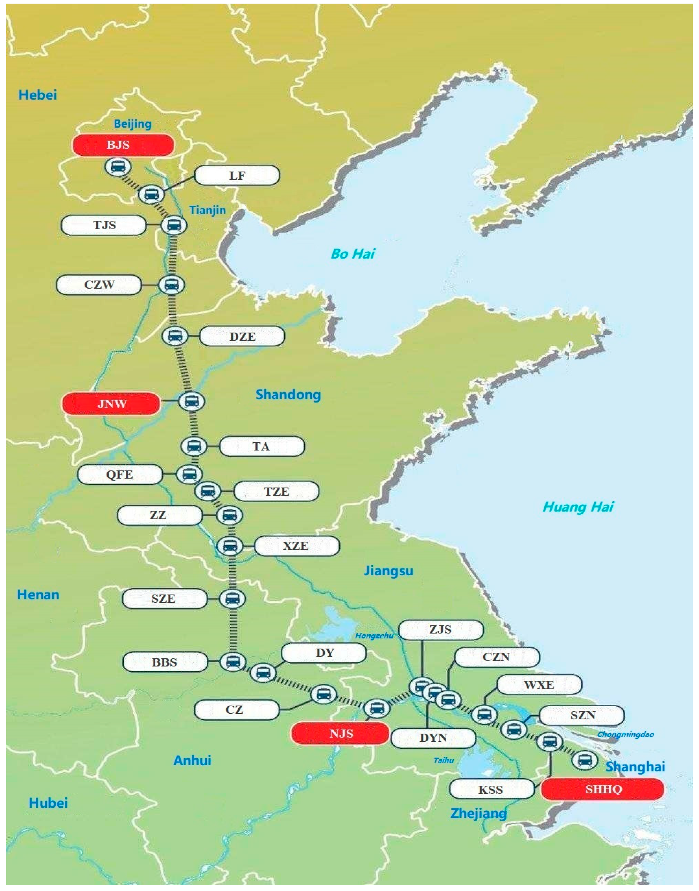
To evaluate the performance of the proposed approach, we present a case study on Beijing–Shanghai HSR Line (
Figure 1), one of the busiest HSR lines in China. It runs a total of 1318 km and is a main N-S railroad corridor in China, including 23 stations and 44 unidirectional sections, where the short names of the stations are illustrated in the figure. The 23 short names are Beijing South (BJS), Langfang (LF), Tianjin South (TJS), Cangzhou West (CZW), Dezhou East (DZE), Jinan West (JNW), Taian (TA), Qufu East (QFE), Tengzhou East (TZE), Zaozhuang (ZZ), Xuzhou East (XZE), Suzhou East (SZE), Bengbu South (BBS), Dingyuan (DY), Chuzhou (CZ), Nanjing South (NJS), Zhenjiang South (ZJS), Danyang North (DYN), Changzhou North (CZN), Wuxi East (WXE), Suzhou North (SZN), Kunshan South (KSS), and Shanghaihongqiao (SHHQ), respectively. The stop time at high-level stations is 3 min, while that at low-level stations is 2 min, which can be properly extended to avoid conflicts. The acceleration/deceleration time is set as 2 min.
The baseline plan is obtained from the data in the third quarter of 2021. The reference line plan consists of the trains running on 3 September 2021, which is adopted as the initial solution to adjust the line plan on 10 September 2021.
The travel demand data is obtained from the ticket sale data, including the original travel demand and the actual travel demand of each O-D pair . There are 96,581 passengers traveling on 3 September 2021, while the travel demand volume on 10 September 2021 grew to 108,990.
- (iii)
Operation parameters
The operation period is from 6:00 to 24:00, km, train, the lower limit of common train proportion , , are 60% and 85%, respectively, and the threshold for trigger decision is 0.1.
- (iv)
Model and algorithm parameters
According to the evaluation of the line plans of the Beijing–Shanghai HSR Line, we set the weights in the model (15): . The algorithm parameters are .
5.2. Performance Analysis
5.2.1. Analysis of Trigger Decision
We make the trigger decision based on the original travel demand and the actual travel demand. We calculate the two coefficients of demand fluctuation by Equations (16) and (17) and , which both exceed the threshold for trigger decision. Thus, the trigger condition is satisfied, then it is needed to make adjustments to the reference line plan.
5.2.2. Analysis of Space-Time Coupled Train Set Partition
Based on the actual travel demand on 10 September 2021, we evaluate the reference line plan (initial solution) by the passenger flow assignment approach in [
1] and [
42] to obtain the operation indexes. Among the diverse operation indexes, the load factor can not only represent the utilization ratio of transit capacity but also show the match degree between the transit capacity allocation and travel demand. Thus, we adopt the load factor as the criterion of space-time coupled train set partition.
Table 1 shows the distribution of train load factors of the reference line plan which represents a relatively uniform distribution, and the average load factor is 67.2%.
According to the lower limit of common train proportion, we sort the trains in the reference line plan by their load factors and select 62 trains to form the fixed train set, then the rest of the trains compose the adjusted train set. In the fixed train set, the average load factor reaches 70.73%, while that of the adjusted train set is only 29.66%.
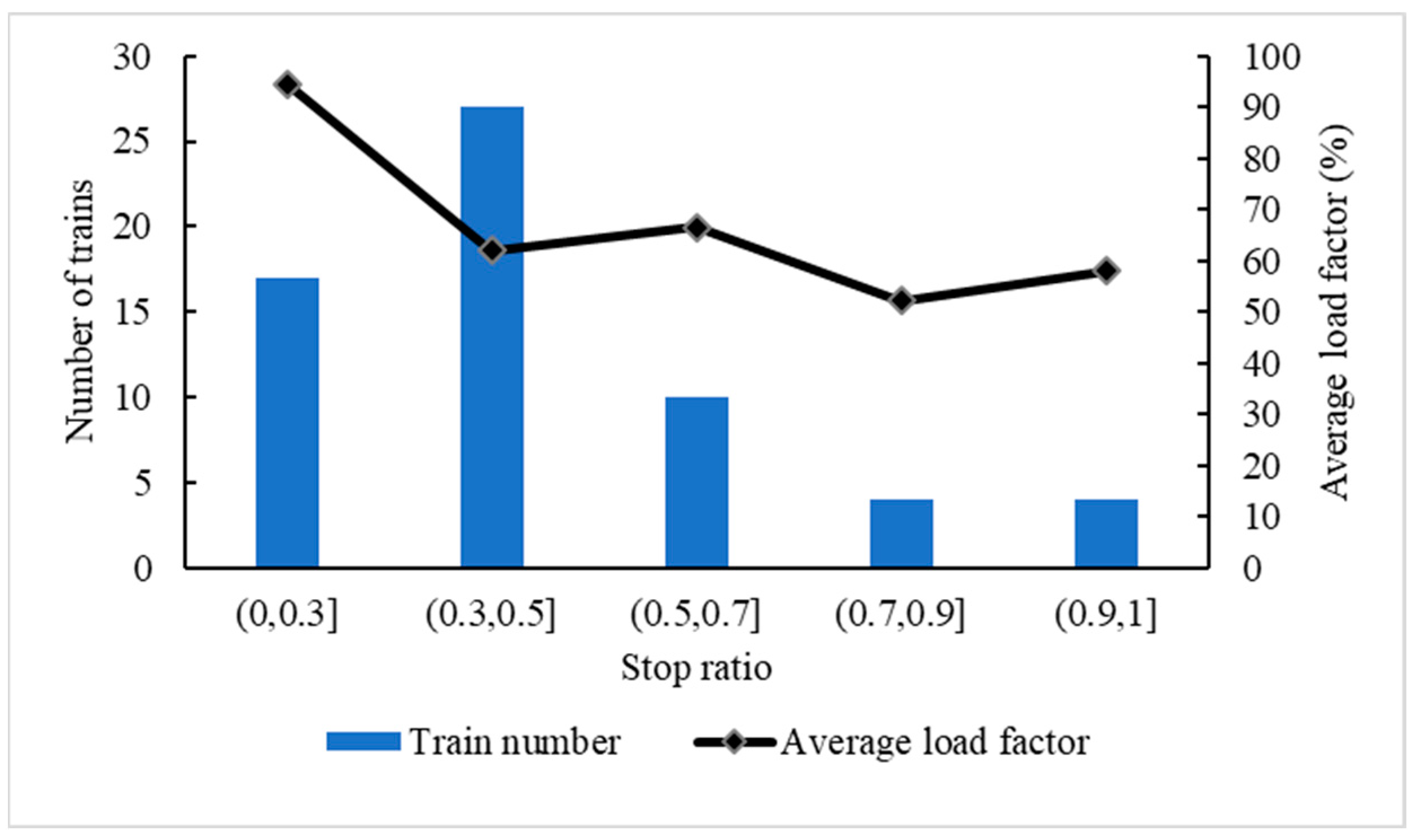
Figure 2 shows the distributions of train numbers and average load factors according to the stop ratios in the fixed train set. It indicates that the stop ratios of most trains in the fixed train set are relatively low (lower than 0.5), which means these trains mainly serve high-level stations with large travel demand volumes and high travel speeds, so the load factors are relatively high. Meanwhile, other trains add more stops to serve the passengers from/to low-level stations with less travel demand and low travel speeds, leading to low load factors.
5.2.3. Comparisons with the Reference Line Plan
We conduct the proposed LPP model in Microsoft Visual Studio 2015 on an Intel i7 2.4 GHZ with 16 GB RAM in the environment of Microsoft Win10. The computation time is 200 s.
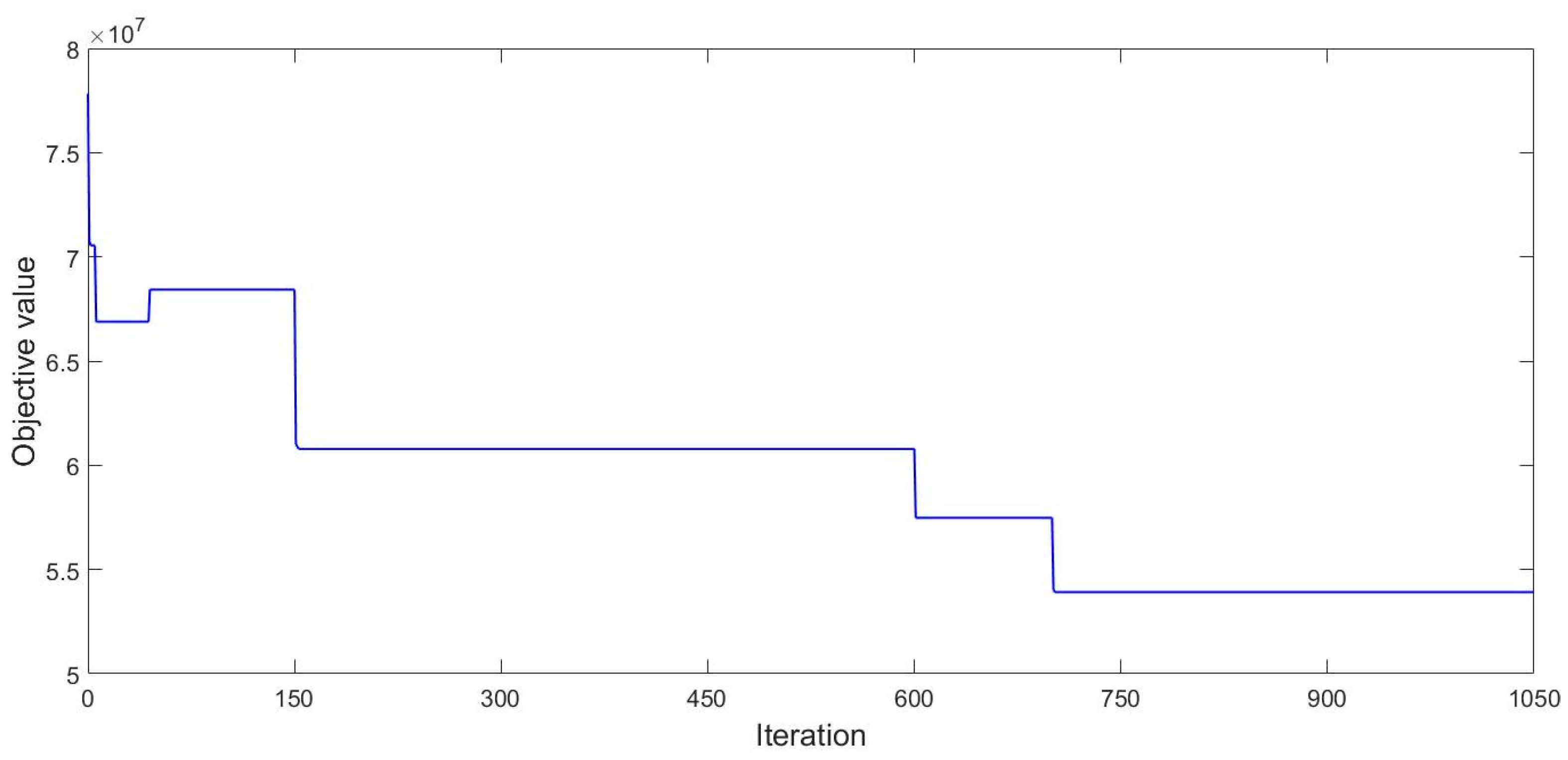
Figure 3 illustrates the convergence process of the objective value. It shows that the objective value reduces from 7.78
107 to 5.39
107, optimizing by 30.72% with a good convergence effect. Next, we make comparisons between the adjusted line plan and the reference line plan.
- (a)
Comparisons of operation indexes
Table 2 shows the comparisons of operation indexes. It indicates the adjusted line plan can obviously reduce the operation cost by comparing the EMU kilometers and train cost. In the optimization process, two trains are deleted from the reference line plan due to low load factors, while other trains are iteratively optimized by adjusting the train elements. The final common train proportion is 97.4%. In the reference line plan, there are 62 long-/coupled-fleet trains and 15 short-fleet trains, and the average load factor is 67.2%; after adjustment, the adjusted line plans have 75 trains with 50 long-/coupled-fleet trains and 25 short-fleet trains, and the average load factor increases to 76.36%. It is shown that the proportions of long-/coupled-fleet trains are both higher than those of short-fleet trains in the two line plans, which means the travel demand on the Beijing–Shanghai HSR Line has huge volume and uniform distributions. Thus, it is proper to operate long-/coupled-fleet trains on this line.
Table 3 shows the distribution of train load factors in the adjusted line plan. Compared with
Table 1, trains with high load factors are obviously more than those in the reference line plan. It indicates that searching strategies can match train operation and capacity allocation, which have the advantage of reducing operating costs.
- (b)
Comparisons of service indexes
Table 4 shows the comparisons of service indexes between the reference line plan and the adjusted line plan. In the adjusted line plan, the TTT, DPK, DPV, and ADT are all lower than those in the reference line plan. It indicates the adjusted transit capacity can better match the travel characters of demand, which is beneficial to reducing travel cost and improving service level. There are 5103 detained passenger kilometers in the adjusted line plan due to capacity constraints, accounting for lower than 0.01%, which means the adjusted line plan can provide sufficient transit capacity. The TMD increases after optimization because the proposed approach devotes to satisfying the travel requirements of passengers, then some transfer and shuttle phenomena would occur, leading to the mileage deviation from the shortest route. The TMD only accounts for 0.23%, which means the adjusted line plan can provide sufficient direct trains to satisfy passengers’ travel requirements.
Table 5 shows the comparison of the mileage distribution of detained passengers between the reference line plan and the adjusted line plan. In the reference line plan, more long-distance passengers are detained due to the unreasonable transit capacity allocation; the adjusted line plan optimizes the transit capacity allocation to better match travel demand, so the detained passengers are all short-/medium-distance passengers who have more travel modes to choose. The ADTs in the two line plans are both around 23 min, meaning passengers can find proper travel schemes within a short boarding deviation time.
Table 6 shows the change in station service frequencies and stop ratios after adjustment. Overall, the changes are slight. The service frequencies for the whole stations all satisfy the required lower limits, and the stop ratios in the adjusted line plan are slightly lower than those in the reference line plan. It indicates that the adjusted line plan rebalances the transit capacity by reducing the stop ratios and adjusting fleet sizes to match the travel requirements of passengers, thereby reducing travel time and improving the attraction to demand.
5.3. Analysis on Space-Time Transit Capacity Allocation
5.3.1. Train Plan Diagram
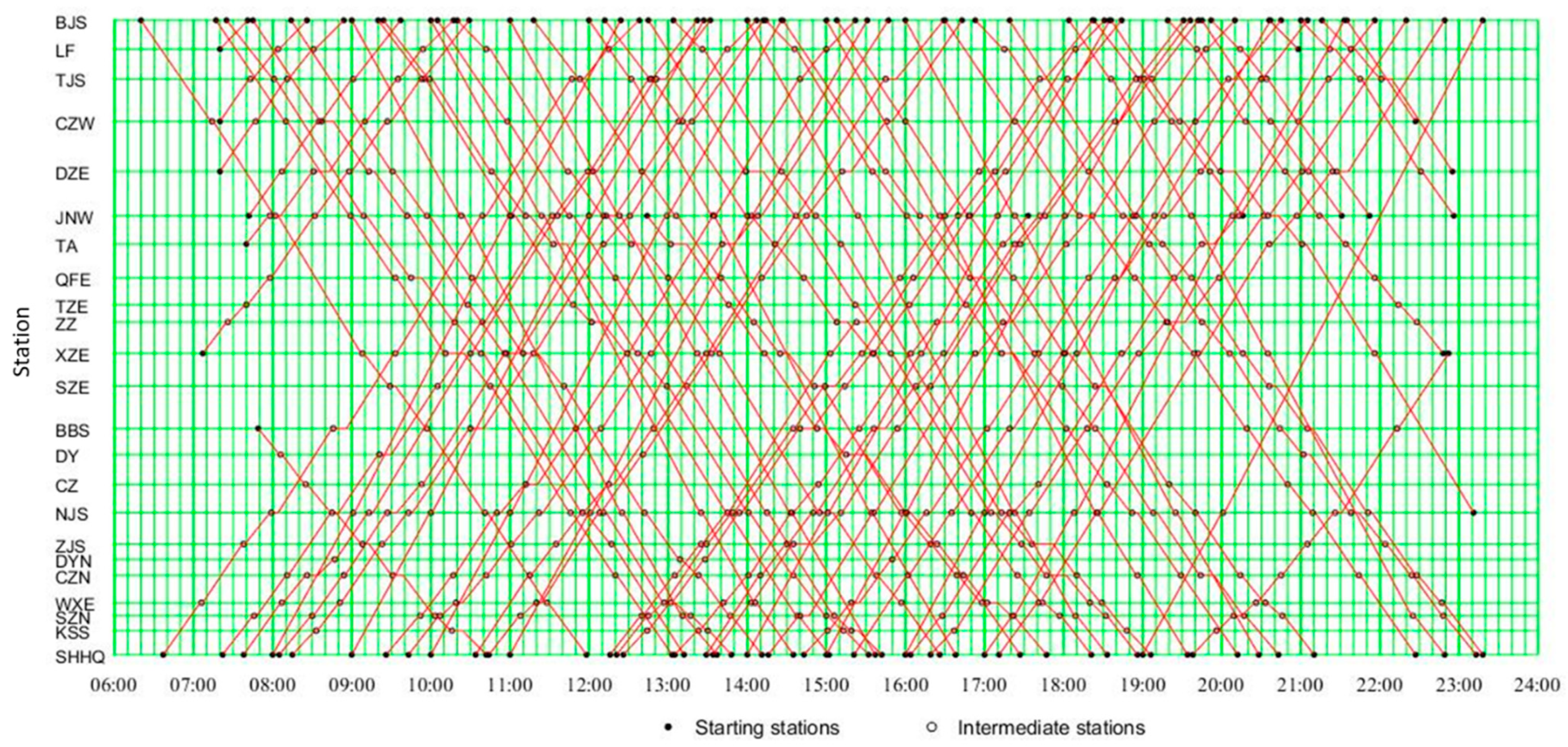
We present the train plan diagram of the adjusted line plan in
Figure 4 to show the train routes, stopping patterns, starting stations, and time information. In
Figure 4, the vertical axis presents the distribution of HSR stations, and the corresponding short names are illustrated (see
Section 5.1), while the horizontal axis presents the operation period of the day. It can also present the space-time distribution of trains during the whole day.
It can be seen that the majority of trains run along the whole line because the uniform distribution of section demand on this line is proper to operate such trains. There are also some regional trains with symmetry characters that distribute around both ends of the space-time zone, which aim to serve the regional travel demand and provide convenience for train circulation.
The length of Beijing–Shanghai HSR Line is 1318 km, and the total travel time along the line is around 6 h, which is suitable for arranging along-line trains with uniform starting times (6:00~19:00). The regional trains distribute the start and end period to serve commute passengers.
As for the station service frequency, there are only starting trains and some regional trains provide service during the early period (6:00~9:00), then the service frequencies for the station increase with time goes on, and the whole station can receive service during 12:00~18:00; because most trains run along the whole line, the number of starting trains gradually decreases after 18:00, and the service frequencies present the dropping trend; during 21:00~24:00, the station service has the symmetry characters with the early period. It shows the station service frequency presents a relatively uniform distribution, indicating that the optimization process can trade off the demand fluctuation characters and the uniformity of station service.
5.3.2. Space-Time Distribution Characters
Based on the HSR network and travel demand, we assign the O-D demand along the shortest paths between O-D pairs on the network to obtain the section flow and make a comparison with the transit capacity allocated for each section.
Figure 5 illustrates the bidirectional transit capacity and section flow along the line, where each section is presented by the short names of two neighbor stations (see
Section 5.1). It can be seen the bidirectional section flow distributions have relatively symmetry characters, where the down direction shows slight increases in the segments, such as BJS-JNW and XZE-NJS. Along the Beijing–Shanghai HSR Line, regional travel demand gathers in the segments including BJS-JNW, JNW-XZE, XZE-NJS, and NJS-SZN.
The bidirectional transit capacity allocations also present symmetry characters, which can satisfy the travel requirements of passengers. The transit capacity utilization ratios of segments at the ends of this line are relatively low and gradually increase in the middle of the line. Most trains run along the whole line and some trains run at the ends of the line, then the transit capacity at the ends would be relatively high, while the section flow at the ends is not accumulated demand, leading to low utilization ratios. In contrast, fewer trains run across the middle of the line, resulting in a lower transit capacity, while the middle section flow is obtained by demand accumulation, so the utilization ratios in the middle of the line are higher.
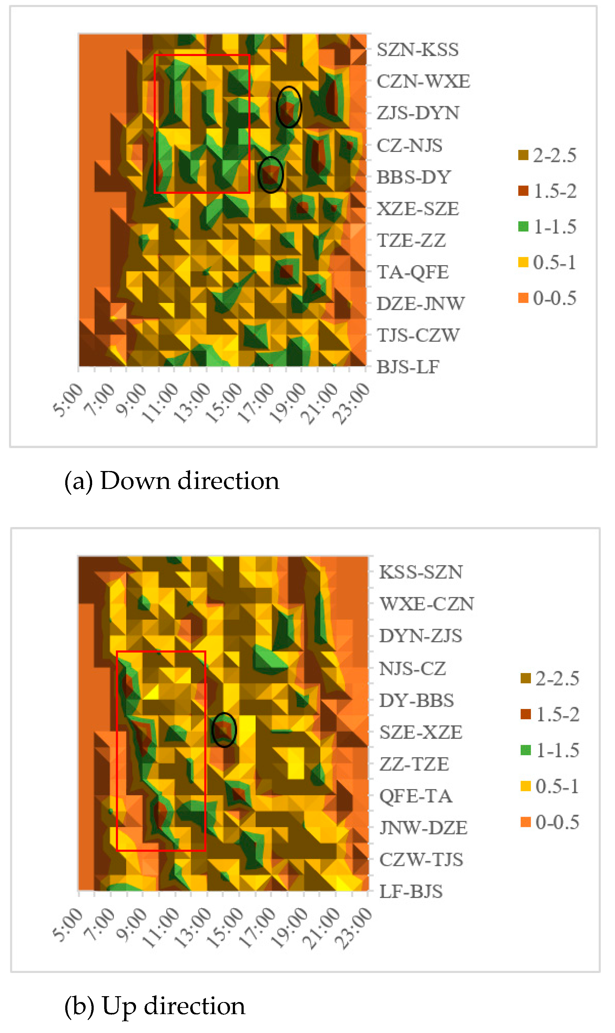
According to the demand intensity distributions and the train plan diagram, we can further obtain the space-time distributions of bidirectional section flow and transit capacity. We define the match degree between transit capacity and section flow, which is the ratio of section flow to transit capacity in each space-time unit. If the match degree is no larger than 1, then the transit capacity can satisfy the travel requirements; otherwise, the insufficient transit capacity cannot satisfy the corresponding passenger flow.
Figure 6 illustrates the space-time distribution of the match degree in the whole space-time operation zone. It can be seen that in the majority of space-time units, the transit capacity can satisfy the corresponding section flow. In some special space-time units, the allocated transit capacity is lower than the section flow. These units can be mainly classified into two categories.
- (i)
Continuous space-time zones with accumulation characters
These zones (red squares) have accumulation characters and generally distribute in the middle of the line. The stations in the middle of the line are generally intermediate stations without starting capacities, so the passenger demand have to wait for the trains starting from other stations, leading to delays in the service interval and accumulated passenger flow.
- (ii)
Single peak space-time units
These units (black circles) are small-range peaks due to demand fluctuation. Because trains all have specific discrete service zones, the continuous section flow in some space-time units cannot be served in time due to load factor requirements and capacity constraints. The remaining passenger flow need to adjust their departure times to board trains with sufficient capacity in neighbor zones.
5.4. Potential Indications of the Proposed Approach
According to the obtained results and analyses, we can obtain some indications and implications of the proposed approach for the practical HSR operation.
- (i)
The proposed approach can not only reduce operation costs and improve service level but also ensure the operation stability. It presents the obvious advantage of reducing operation cost.
- (ii)
High-quality trains generally have low stop ratios and high travel speed to attract more passenger demand. Operators can reasonably adjust the stop distributions of trains to rebalance the transit capacity allocation.
- (iii)
The space-time transit capacity allocation obtained by the proposed approach can satisfy the travel demand, except for some space-time units caused by practical reasons where the detained passenger demand can adjust their travel to receive travel service.
6. Conclusions
In this paper, we propose an approach of daily line planning optimization to trade off the system costs and the operation stability. The adjusted line plan is obtained by adjusting the reference line plan based on the baseline plan. A bi-level programming model is established based on Stackelberg game theory to describe the interaction and conflicts between railway companies and passengers, which incorporates the line planning adjustment and evaluation feedback. The concepts of space-time segment candidate set and common train proportion are adopted to ensure operation stability.
The daily line planning problem is solved under the SAA framework, involving trigger decision, space-time coupling, and joint iteration. The trigger decision is executed to determine whether to make adjustments and then the fixed train set and adjusted train set are classified according to evaluation on the reference line plan. Several neighborhood searching strategies are proposed to adjust train elements according to the evaluation results.
The adjusted line plan can not only optimize the system costs but also ensure the operation stability. It presents the obvious advantage of reducing operating costs and can also rebalance and provide sufficient transit capacity for passengers to improve service level and attraction to travel demand. The uniform distribution of passenger demand makes it suitable to set along-line trains with uniform starting times. As for the detailed space-time distribution, the transit capacity of most space-time units can satisfy the corresponding section flow, except for the special zones caused by station location and load factor requirements. By adopting the proposed approach, the optimized system costs and operation stability can improve resource utilization and benefit positive daily operation sustainability in railway systems. It is an effective technique for reaching sustainable railway operations and organizations.
Our future research can be extended in several aspects. First, we need to consider more practical factors in line planning optimization to realize more practical line plans, such as train circulation, coupling between in-line trains and cross-line trains, and the trade-offs between network operation and regional operation. Second, we can further investigate conflict resolution in line planning to improve the feasibility of line planning. Third, energy consumption is also a good research direction for line planning, and we can optimize the train speed profile to reach energy-saving goals.


