Sustainability Oriented Vehicle Route Planning Based on Time-Dependent Arc Travel Durations

Abstract

Traffic congestion has become a growing concern in cities, with both economic and environmental impacts on both individuals and the logistics industry. Therefore, a model of freight distribution in urban areas considering economic and environmental objectives needs to be established to alleviate the consequences. In this paper, a multi-stage heuristic algorithm is designed for solving the route planning based on time-dependent arc travel durations. The algorithm includes a savings method, a modified tabu search heuristic and a cycle transforming optimization (CTO) algorithm. Benchmark instances and the case of Jingdong, one of the largest e-commerce platforms in China, have been adopted to verify the accuracy and feasibility of the model and algorithm. Results of the performance test reveal that the designed algorithm is suitable for addressing large-scale instances. Based on the single objective models, two objectives referring to economical-related and environmental-related factors are considered in the proposed sustainability oriented bi-objective model, and a modified solution framework using a multi-objective decision making method with a relaxation coefficient which is designed for addressing the bi-objective model. Finally, the time-dependent arc travel durations based on real-time traffic information have been incorporated into the optimization algorithms, simulation of distribution process and dynamic route updating strategy, which can reduce costs and route-associated emissions of logistics companies.

1. Introduction

Efficient distribution and/or collection plays a significant role in urban logistics. To date, traffic congestion has been seriously affecting the development of urban logistics. For instance, bakeries need to deliver a variety of products to their shops or franchisees distributed throughout the city and collect the bread that is about to expire. On school days, school buses need to collect or send students from different communities on time, and large-scale supermarket chains need to deliver goods from the warehouse to the store. Route planning can improve transportation efficiency, cost saving and emission reduction [1]. In short, sustainability-oriented vehicle route planning in urban areas is a challenging and meaningful research topic.

Cities with a variety of high-quality resources attract a large number of people. An increasing number of citizens leads to the rapid rise in travel and logistics demand. Due to the limited transportation resources, traffic congestion occurs in the urban road network frequently. The time-dependent characteristics of traffic congestion have an important impact on the cost of urban logistics. For example, time-dependent travel durations affect vehicle speed, which in turn influences distribution cost. At the same time, the closer to the urban core, the more carbon emissions arise. The carbon emission is proportional to gross domestic product (GDP) per capita. Therefore, it is necessary to consider the impact of vehicles on the environment in the route optimization of urban logistics. The sustainable development of urban logistics includes economic factors and environmental aspects. The enterprise of urban logistics focuses on reducing the operational costs and impact of distribution vehicles on the environment through optimization models and algorithms.

This study focuses on providing a general methodology that contributes to the solution of urban logistics. Our methodology includes a calculation method of time-dependent arc durations, capacitated vehicle routing problem (CVRP) models, multi-stage heuristic algorithms, a simulation method, and a dynamic route updating strategy. The utilizing of the simulation method and dynamic route updating strategy is conducted to achieve sustainability-oriented vehicle routing planning in urban areas.

The residual parts are organized as follows: Section 2 is the literature review focusing on vehicle routing problems (VRP) and its variations. In Section 3, we present a formal description of the problem to be investigated as well as the calculation method of time-dependent arc durations in detail. Section 4 introduces two models with economic objective or environmental objective, respectively, and the detailed process of the multi-stage heuristic algorithm and the solution framework for bi-objective models are described in Section 5. The performance test of the multi-stage heuristic algorithm is implemented in Section 6. Section 7 includes a case study of a supermarket daily delivery. Finally, this study has been concluded in Section 8.

2. Literature Review

The literature review starts with the existing exact algorithm and heuristic algorithm. Then, the research focusing on time-dependent vehicle routing problems (TDVRP) is introduced. Finally, the studies closely related to sustainability-oriented vehicle routing problems are analyzed in objectives and solution methods.

A large number of exact algorithms have been developed for solving models related to CVRPs and its variants. Letchford et al. [2] proposed the first exact algorithm for the open version of the CVRP based on branch-and-cut (BC). Christiansen and Lysgaard [3] introduced a new branch-and-price (BP) algorithm for CVRP considering stochastic demands. The algorithm included the branch-and-bound and column generation subproblem. Xie et al. [4] established a multimodal hazmat location and routing model, and converted the model into a mixed integer linear program for using the CPLEX or other exact solvers. Gauvin et al. [5] proposed a branch-cut-and-price (BCP) algorithm for the vehicle routing problem with stochastic demands. Santos et al. [6] presented a BCP algorithm for the two-echelon vehicle routing problem. Dinh et al. [7] applied BCP and dynamic programming to solve the chance-capacitated vehicle routing problem. Munari et al. [8] proposed a BCP method based on a set partitioning formulation of the robust vehicle routing problem with time windows, which relies on the resource-constrained elementary shortest-path problem. Aiming at the vehicle routing problem with stochastic demands under optimal replenishment, Florio et al. [9] proposed a BCP algorithm that relies on an efficient labeling procedure, many dominance rules, and completion boundaries to column generation. Xiao et al. [10] constructed a linear programming model based on ε-accurate method, and the experimental results showed that the AMPL/CPLEX can solve the benchmark test instance of vehicle routing problems with a maximum of 25 clients. Based on a modified label setting algorithm, Zhang et al. [11] developed a BP algorithm to solve the shared autonomous electric vehicle routing problem.

Closely related to the algorithm designed in this study are the savings method and tabu search algorithm. The former was proposed for a larger truck dispatching problem [12], the results revealed that it was able to quickly obtain good solutions during the iterative process in a limited time. Since then, the algorithm has been widely developed and applied. Given that solutions generated by the savings method have a larger gap compared with the best solution, it needs to be further optimized, and a large number of works have used the tabu search algorithm to do so. Zidi et al. [13] designed a hybrid simulated annealing tabu search algorithm to provide an effective routing selection method for ambulances. The experimental results showed that the proposed algorithm performed better than the particle swarm optimization (PSO) and the genetic algorithm and exhibited less time consumption. Omidvar et al. [14] developed a two-phase model to solve time-dependent vehicle routing and scheduling problems. A mixed-integer programming model dealt with speed variations in road networks and generated a fixed node sequence for each route in the first phase, then the departure time of each fixed route was rearranged to avoid traffic jams as much as possible in the second phase. Combined with the multiple phase neighborhood search algorithm and greedy randomized adaptive search algorithm, a hybrid PSO algorithm was designed to deal with supply chain management problems [15]. Rong and Xu [16] developed a Stackelberg game analytical framework to obtain the stakeholder’s optimal solutions for green supply chain management. Akeb et al. [17] developed a multi-stage heuristic algorithm to solve the capacitated vehicle routing problem with time windows (CVRPTW). The three stages included clustering customers (grouping), constructing routes and intensification.

Various time-dependent functions between vehicle speed and departure time have been introduced in the TDVRP. Ichoua et al. [18] proposed time-dependent travel speeds with the “first-in-first-out” property to further enrich the TDVRP and considered many factors such as time of the day and different vehicle speeds. Lecluyse et al. [19] proposed a parallel tabu search algorithm for a static and dynamic TDVRP case. Jabali et al. [20] established a TDVRP model considering travel time, fuel consumption and CO₂ emission cost. The carbon emission was reduced by limiting vehicle speed and avoiding driving in peak hours. Qian and Eglese [21] considered time dependence and vehicle speed as decision variables to establish the vehicle routing problems with minimizing total greenhouse gas emissions, and adopted a column generation algorithm based on tabu search for verification in real cases. Cimen and Soysal [22] proposed a Markov decision model and used heuristic algorithms of approximate dynamic programming to solve TDVRP. Aiming at minimizing carbon emissions and total cost, Wang et al. [23] proposed a hybrid heuristic algorithm based on the savings method, scanning algorithm and multi-objective particle swarm optimization algorithm to solve the multi-depot vehicle routing problem with time-varying speeds. Huang et al. [24] regarded the problem of route selection as a kind of comprehensive decision in TDVRPs and established a TDVRP-path flexibility model under deterministic and random traffic conditions. Combined the order selection problem with TDVRP, Ma et al. [25] introduced an optimization model considering the delivery order, service order and the start time of the delivery task, and proposed an ant colony algorithm with local search operators. Fan et al. [26] proposed a hybrid metaheuristic algorithm to solve the time-dependent multi-depot vehicle routing problem. Combined the greedy randomized adaptive search procedure (GRASP) with the iterated local search (ILS), Allahyari et al. [27] designed a hybrid algorithm for solving the secure TDVRP considering time-dependent travel speeds. Recently, Schmidt et al. [28] proposed a metaheuristic based on an evolutionary search for the time-dependent fleet size and mix multi-depot vehicle routing problem. The modeling of sustainability-oriented vehicle routing problems mainly considers economic factors, environmental impacts or customer satisfaction, etc. Costa et al. [29] investigated a bi-objective green vehicle routing problem with time windows in which the minimization of CO₂ emission costs conflicts with the optimal economic cost of total driver wage that is associated with each passed unit of time. Poonthalir and Nadarajan [30] established a bi-objective green vehicle routing problem with variable speed constraints considering the minimization of path cost and fuel consumption, and designed a particle swarm optimization algorithm with greedy mutation operator to solve the problem. Zhao et al. [31] studied the time-varying bi-objective vehicle routing problem with time windows. The proposed mixed integer linear programming model with minimizing total transportation cost and time cost was solved by non-dominated sorting genetic algorithm (NSGA-II). Zhou et al. [32] proposed a NSGA-III algorithm with simulated annealing for the multi-objective waste collection routing problem. The economy, society, and environment objectives were considered for sustainable development of cities. Aiming at the multi-objective heterogeneous vehicle routing problem, Ghannadpour and Zarrabi [33] presented a bi-objective model based on fuel consumption and customer service priority to ensure the minimization of total vehicle driving distance, fleet size, fuel consumption and the maximization of customer satisfaction. Ren et al. [34] studied a mixed-energy fleet green vehicle routing problem with minimizes pollutant emissions and the total delay time. A modified variable neighborhood search algorithm with a selection mechanism was presented to find the Pareto frontier of the bi-objective model. Islam et al. [35] proposed a new hybrid PSO algorithm to deal with the mixed-fleet-based green clustered logistics problem under carbon emission cap in logistic industry. Amiri et al. [36] established a bi-objective model minimizing total cost and carbon emissions, and designed three multi-objective solutions (linear weighted sum, ε-constraint and hybrid method) based on the adaptive large neighborhood search (ALNS) algorithm. Glize et al. [37] introduced a ε-constraint method for the bi-objective vehicle routing problem based on column generation and enumeration algorithm. Zarouk et al. [38] constructed a bi-objective model for minimizing energy consumption and maximizing customer satisfaction and proposed a hybrid metaheuristic algorithm based on genetic algorithm and simulated annealing algorithm.

On the basis of the existing works mentioned above, four weaknesses can be found as follows. (a) Large-scale cases in real-world applications cannot be solved by exact algorithms in a reasonable time because the algorithms are time-consuming even when performing on small-scale instances. (b) Although the previous studies have solved the TDVRP in different ways, there is a significant research gap, i.e., few of them consider the real traffic information of target areas. (c) Common algorithms for solving bi-objective or multi-objective vehicle routing problems include multi-objective particle swarm optimization algorithm, multi-objective evolutionary algorithm and ε-constraint method. There are few works using multi-objective decision making methods. (d) Most of the existing work of vehicle routing problems focus on the theoretical optimization, and there are few application studies on whether the distribution scheme can be successfully fulfilled in the road network of the target area and how to fulfil it.

To fix the above weaknesses, a fast multi-stage hybrid heuristic algorithm is designed, which includes the savings method, the tabu search algorithm and the cycle transforming optimization algorithm. Based on the basic road network data and real-time traffic information of the target area, a segmental time-dependent arc travel duration calculation method is presented to address the time-dependent parameters in the vehicle routing problem. Meanwhile, a multi-objective decision making method with relaxation coefficient is used to solve the bi-objective problem. By adding constraints and control relaxation coefficient to the problem, the algorithm for solving the single-objective problem is transformed into the algorithm for solving the bi-objective or multi-objective problems. A simulation method and a dynamic route updating strategy are designed to verify whether the distribution scheme can be implemented and how to implement in the road network of the target area.

Based on the above analysis, this study focuses on the extension of providing efficient routes for freight distribution in urban areas. The contributions of this paper are summarized as follows:

• The establishment of a multi-stage heuristic algorithm to solve single-objective vehicle routing problems;
• The proposal of multi-objective decision-making method with relaxation coefficient to solve bi-objective or multi-objective vehicle routing problems;
• The design of a time-dependent arc duration calculation method and applying it to the optimization algorithms and simulation method;
• The development of a simulation method and dynamic route updating strategy.

3. Problem Description

3.1. Formal Description

In the investigated vehicle routing planning based on time-dependent arc travel durations, the locations of customers and depot and their corresponding relationship are modeled in a graph G = (V, A), which consists of a node’s set V and of an arc’s set A. Assuming the arc length $(i,j)=(j,i),\forall i,j=V$, the routing problem is referred to as undirected case, otherwise, it is called directed case. Each arc can be assigned a weight that may represent the corresponding travel distance and time-dependent travel duration. In addition, each customer has a request q, and development of optimization algorithms aims to meet the demands of customers with the minimum cost and emission by assigning deliver vehicles from the depot. This paper focuses on the undirected cases for benchmark instances and directed cases for practical scenario.

3.2. Time-Dependent Arc Durations

The time period T is equidistant divided into H time slots by time interval $\gamma$, that is to say, the continuous time range T is discretized into H time slots. Assuming the starting time is $t_0$, the time range T can be expressed as $T=\{t_0,t_0+\gamma ,\dots ,t_0+H\gamma \}$.

Let $T_h,h\in 1~H$ denote the number of slots, each time slot can be represented as a time range $[t_h,t_{h+1}]$, where $t_h$ is the start time and $t_{h+1}$ is the end time of the time slot $T_h$ Assume that $s_{ij}^h$ represents a time-dependent travel velocity of the arc $(i,j)$ in the time slot $T_h$, and vehicles pass through arc $(i,j)$ in a sequential mode (FIFO) between nodes i to j, in which several consecutive time slots could be consumed. Then, the piecewise linear function ${\tau }_{ij}(t)$ is defined to calculate the time-dependent arc durations.

$${\tau }_{ij}(de{p}_i(t))=\{\begin{array}{l}{L}_{ij}/s_{ij}^{h_a},if h_a=h_b\\ ar{r}_j(t)-ar{r}_i(t),if h_b=h_a+1\\ (t_{h_a+1}-ar{r}_i(t))+(h_b-h_a-1)\gamma +(ar{r}_j(t)-t_{h_b}),if h_b>h_a+1\end{array}$$

(1)

In Formula (1), $h_a$ and $h_b$ denote the depart slot and arrival slot, respectively, $ar{r}_i(t)$ represents the arrival time of the vehicle at node i. Without considering the service time of nodes, the arrival time at node i is equal to its departure time, i.e., $ar{r}_i(t)=de{p}_i(t)$. Then, Formula (1) is described below in detail.

(a)

If $h_a$ and $h_b$ in the same time slot, the time-dependent velocity on the arc is equivalent, and the time-dependent arc duration is the ratio of the distance L_ij to the time-dependent velocity $s_{ij}^{h_a}$.

(b)

If $h_a$ and $h_b$ within two adjacent time slots, the travel duration spans two time slots. The calculation method of time-dependent arc durations is illustrated in Figure 1a.

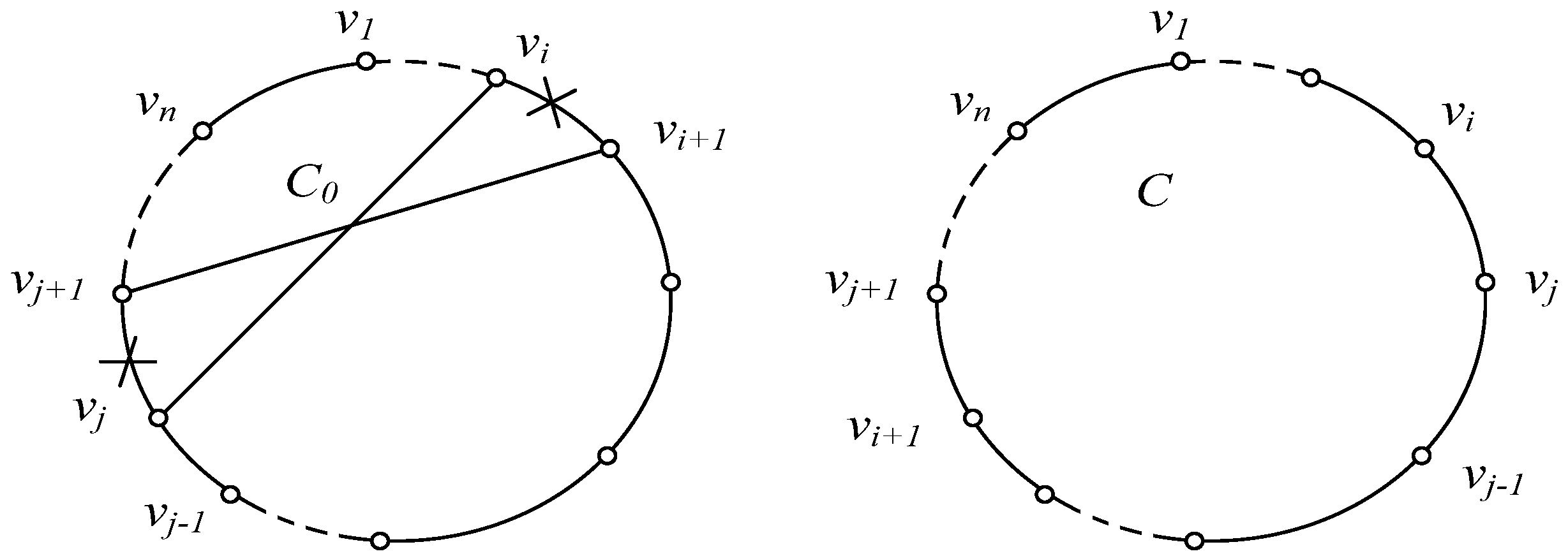
As can be seen from Figure 1a, arc length L_ij is divided into two segments, and the arrival time at node j from i is: $ar{r}_j(t)=ar{r}_i(t)+L_{il}/s_{il}^{h_a}+L_{lj}/s_{lj}^{h_b}$.

(c)

If $h_a$ and $h_b$ in two non-adjacent time slots, the travel duration on arc (i, j) is composed of three parts, as illustrated in Figure 1b. The first part is equal to the start time of time slot subtracting the start time of the node i. The second part contains a number of complete time slots. The third part is equal to the arrival time of the node j minusing the start time of the time slot $h_a+1$. As can be seen from Figure 1b, arc length L_ij is divided into n + 1 segments, and the arrival time at node j from i is: $ar{r}_j(t)=ar{r}_i(t)+L_{i{l}_1}/s_{i{l}_1}^{h_a}$ $+\left(n-1\right)\gamma +L_{l_{n}j}/s_{l_{n}j}^{h_b}$.

The parameter L_ij denotes the actual driving distance provided by the online map platform application program interfaces (APIs). The speed s_ij of each time slot is calculated by the basic data of road networks under the free flow state and traffic performance index (TPI). By continuously capturing data from the online map platform, the TPI of each time slot in the future can be predicted by deep learning methods to achieve full coverage of the time slot in the distribution process.

4. Problem Formulation

Two models are established separately based on the traditional CVRP model. Model 1 is to minimize the total travel distance, which satisfies the business objectives of urban logistics enterprises. Model 2 represents the minimization of total emissions, which meets the regulatory requirements of governments. Although the two models have the same constraints, they represent the interests of different participants. Model 1 represents the interests of logistics enterprises, whereas Model 2 represents the government’s environmental concerns.

4.1. Model 1

This model aims to minimize the total distance by using two sets of constraints related to vehicles, i.e., the capacity and maximum range. A three-index vehicle flow model for minimizing the total distance including a summation of the selected arc lengths is defined by:

$$Min{z}_1={\displaystyle \sum _{i=0}^n{\displaystyle \sum _{j=0}^n{\displaystyle \sum _{k=1}^m{d}_{ij}}{x}_{ijk}}},$$

(2)

where d_ij is equal to L_ij in Formula (1). The capacity constraints in Formula (3) indicates that the total amount of distribution tasks undertaken by the vehicle is not greater than its maximum capacity:

$${\displaystyle \sum _{i=1}^n{q}_i}{y}_{ik}\le Q,\forall k\in K$$

(3)

Constraints (4) ensure that the total distance of each route cannot exceed the maximum range of the vehicle:

$${\displaystyle \sum _{i=0}^n{\displaystyle \sum _{j=0}^n{d}_{ij}{x}_{ijk}}}\le L,\forall k\in K$$

(4)

Although the range of internal-combustion vehicles can be considered as unlimited, it should be regarded as an important factor with the popularization of new energy vehicles in the near future. Constraints (5) means that each customer is serviced by exactly one visit of a single vehicle:

$${\displaystyle \sum _{k=1}^m{y}_{ik}}=1,\forall i\in C$$

(5)

Each vehicle needs to start from and return to the distribution center according to:

$${\displaystyle \sum _{k=1}^m{y}_{0k}={\displaystyle \sum _{k=1}^m{y}_{k0}}=m}$$

(6)

The relationship between two kinds of decision variables is defined by constraints (7) and (8):

$${\displaystyle \sum _{i=0}^n{x}_{ijk}}=y_{jk},\forall j\in V ,k\in K$$

(7)

$${\displaystyle \sum _{j=0}^n{x}_{ijk}}=y_{ik},\forall i\in V,k\in K$$

(8)

The simple sub-tour elimination constraints are defined by:

$${\displaystyle \sum _{i\in S}{\displaystyle \sum _{j\in \left\{V\backslash S\right\}}{x}_{ijk}\ge y_{hk},\forall S\subseteq C ,h\in S,k\in K}}$$

(9)

Two sets of decision variables are given by:

$$x_{ijk}\in \{0,1\}\forall i,j\in V,i\ne j,k\in K$$

(10)

$$y_{ik}\in \{0,1\}\forall i\in V,k\in K$$

(11)

4.2. Model 2

The objective z₁ in Formula (2) ensures the lowest total distance of the solution. However, responsible logistics enterprises, as an important part of urban infrastructure, not only focus on minimizing their cost but also devote to mitigate the negative environmental impacts. To this end, another objective z₂ is defined and the constraints are the same to Model 1.

$$Min{z}_2=EF\cdot {\displaystyle \sum _{i=0}^n{\displaystyle \sum _{j=0}^n{\displaystyle \sum _{k=1}^m{d}_{ij}\cdot f(\frac{d_{ij}}{t_{ij}}})\cdot x_{ijk}}}$$

(12)

The objective represents minimizing the total carbon emission of distribution vehicles, in which the time-dependent travel duration $t_{ij}$ can be calculated by Formula (1) under a specific depart time. Meanwhile $f(\cdot )$ refers to regression functions defined in the computer program to calculate emissions from road transport (COPERT) model [39,40].

The COPERT is a method to estimate emissions for various types of vehicles on the road network. The method requires only a small amount of input data and can achieve accurate emission assessment for fuel vehicles. In addition to assessing carbon dioxide emissions, COPERT can also calculate emissions of four major pollutants, namely carbon monoxide, nitrogen oxides, volatile organic compounds and particulate matter. Meanwhile, the method uses a large number of actual activity data to construct emission factor functions for these substances. The key activity data include the number of vehicles in different emission categories/technologies, vehicle speed on different highway conditions (urban or rural), and the number of miles travelled under the same driving conditions, many other emission evaluation models are published except for the COPERT model. The COPERT model is adopted in this paper to calculate emission factors of carbon dioxide because the raw data it analyzed comes from the real-world intelligence traffic information system and the emission standard of vehicles used in the case study belongs to Euro III that is clearly pre-defined in the COPERT model.

Model 1 belongs to the mixed integer linear programming model and can be solved directly by off-the-shelf commercial solvers such as CPLEX. Unfortunately, the CPLEX solver becomes powerless when facing the large-scale instances (n > 18) because constraints (9) contain an exponential operation to enumerate all subsets of the set C. Model 2 is a mixed integer nonlinear programming model because of a nonlinear objective function contained. Therefore, a multi-stage heuristic algorithm is designed in the next section.

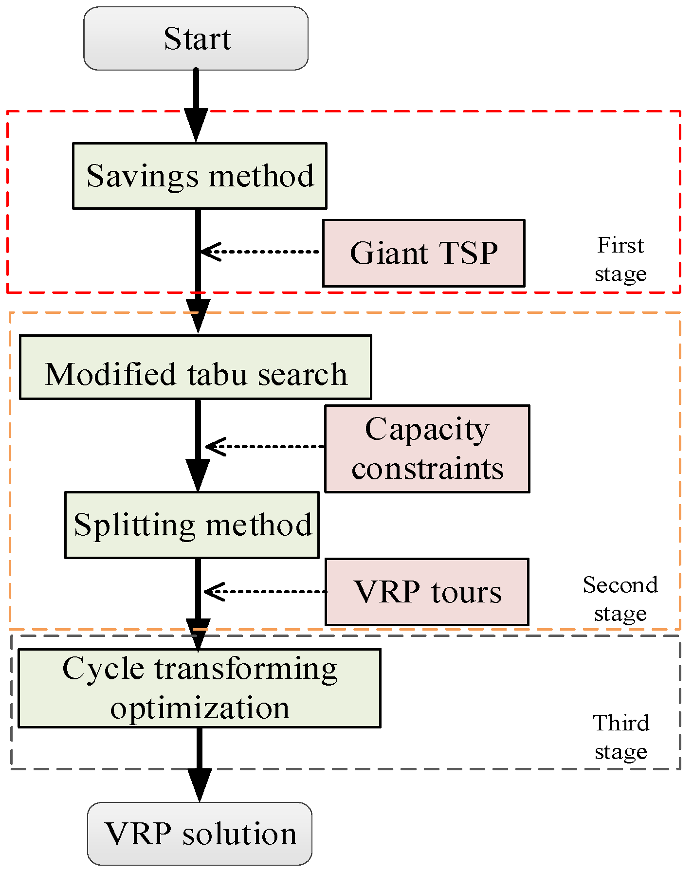
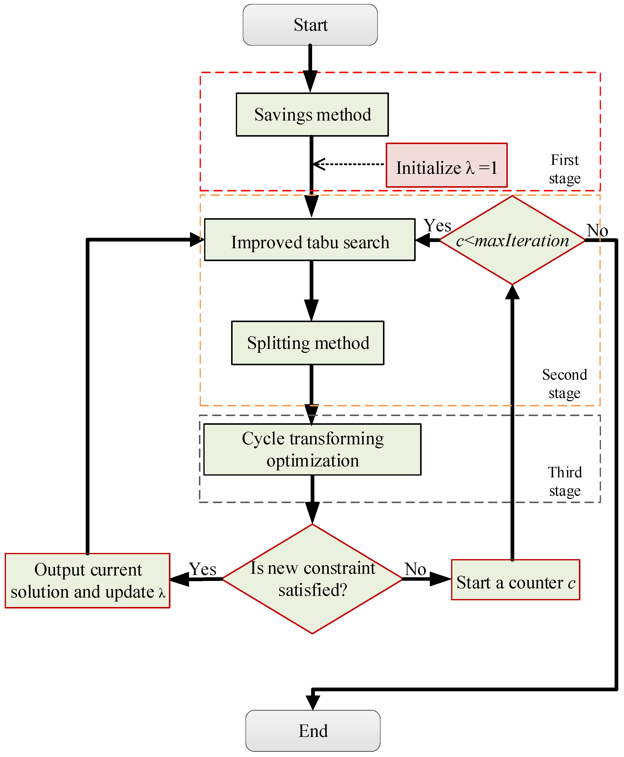
5. Solution Algorithm

The process of the multi-stage heuristic algorithm is shown in Figure 2. The first stage is to obtain a giant traveling salesman problem (TSP) tour by means of the savings method; the second stage is to perform a modified tabu search on the giant TSP tour and output a new one, and then this new giant TSP tour is split into multiple small TSP tours according to the capacity constraints; in the last stage, the small TSP tours representing each vehicle route are intensified by the CTO algorithm, separately.

5.1. First Stage: Savings Method

The principle of Clarke and Wright’s savings heuristic algorithm (CW) is to combine the two sub-tours in the transportation process into one tour [12]. Each combination is to reduce the total transportation distance as much as possible. The new vehicle is used until the loading of the current vehicle is full. The CW generates the distribution plan that minimizes the total travel distance according to the transportation capacity of the distribution center and the distance between the distribution center and customers. Meanwhile, the following constraints should be considered during the optimization process, i.e., all demands of customers, no vehicle is overloaded and the total daily operating time or mileage of each vehicle does not exceed the specified limit.

Natural numbers are used to encode nodes in this paper. During the execution of the first two stage heuristics, the depot is considered as a normal node and finally generates an optimized TSP tour. To increase the search space and to fully account for the performance of modern computers, the capacity constraints are temporarily relaxed in the first stage and second stage. The savings method used in this paper is shown in Figure 3.

5.2. Second Stage: Modified Tabu Search Algorithm

The tabu search was first proposed as a meta-heuristic for guiding and controlling heuristics, and five main concepts are included—initialization, moving and neighborhood, a tabu list, aspiration criteria and termination conditions [41]. A modified tabu search with four neighborhood operators based on node-exchanging is proposed in this paper. The detailed description of the modified tabu search algorithm is described in Algorithm 1.

Algorithm 1: Pseudo-code for the modified tabu search

1: Input X: a result of the CW   2: Preprocessing   3: Set the parameters e.g.history optimal solution (best), current solution (current)   4: Initialize counter: iteration, stop   5:While iteration < MAXiter and stop < MAXstop   6: For i = 0 to M   7:  Randomly select a move operator and generate a new solution X*   8:  Add X* to candidate list TL   9: End For   10: Sort the candidate list by fitness   11: If TL (1) < best Then   12:  stop = 0   13:  Update parameters   14:  If Tabu list not full Then   15:    Add best to Tabu list   16:   Else:   17:    Pop the first item of Tabu list   18:    Add best to the rear of Tabu list   19:   End If   20:  Else:   21:  stop = stop + 1   22:  search current from the Tabu list   23:  update the Tabu list   24:  End If   25:  iteration = iteration + 1   26: End While   27: Output Current solution

In each iteration, candidate solutions are obtained by randomly selecting a neighborhood operator, and the candidate with the minimum objective is added to the tabu table. Because the tabu search is sensitive to the quality of initial solution, a good initial solution can make it converge quickly. For this reason, CW is utilized to generate initial solution obtained in advance.

Inspired by the variable neighborhood search algorithm, the four neighborhood operators, the inverse neighborhood search operator, 1-opt insert search operator, 2-opt* exchange search operator and 3-opt exchange search operator, are designed. The operators are introduced as follows and illustrated in Figure 4.

(a)

Inverse neighborhood search operator: that is, randomly selecting a segment of route and reverse its order;

(b)

1-opt insert search operator: randomly selecting a node inserted into another location in the route;

(c)

2-opt* exchange search operator: randomly selecting two nodes to swap;

(d)

3-opt exchange search operator: randomly selecting three nodes to reassign its location.

The optimized TSP tour obtained by the modified tabu search is split into VRP solutions by using a liner splitting method [42].

5.3. Third Stage: Cycle Transforming Optimization Algorithm

The large number of experimental results show that the results outputted by the TS are worse than the optimal result. Therefore, it is necessary to perform further optimization after dividing a giant TSP tour into a VRP solution. The following two concepts in graph theory are presented for the sake of introducing the CTO algorithm.

Definition 1.

The Hamilton cycle with the smallest weight is the optimal H-cycle in a weighted graph G = (V, E), and the closed path with the minimum weight covering each vertex exactly once is the optimal TSP tour.

Definition 2.

Let $x,y,z\in V,z\ne x,x\ne y$, and if $w\left(x,y\right)\le w\left(x,z\right)+w\left(z,y\right)$ in a weighted graph G = (V, E), then the optimal H-cycle of G is also the optimal TSP tour.

These two definitions show that the optimal H-cycle of graph G is also the optimal TSP tour when the distance between nodes satisfies the triangle inequality [43]. However, solving both the optimal H-cycle and the optimal TSP tour are NP-hard problems, and there is no quick and exact solution algorithm at present, although this can be solved by the CTO algorithm. After obtaining the VRP solution with the modified TS algorithm designed in Section 5.2, the CTO algorithm is performed on each TSP tour to intensify the solution quality. The core of the CTO algorithm is illustrated in Figure 5.

The steps for conducting CTO algorithm are as follows:

Step 1 Take any initial TSP tour, $C_0=v_1,v_2,\cdots ,v_i,\cdots ,v_j,\cdots ,v_n,v_1$.

Step 2$\forall i,j,1<i+1<j<n$ if $w\left(v_i,v_j\right)+$ $w\left(v_{i+1},v_{j+1}\right)<$ $w\left(v_i,v_{i+1}\right)+w\left(v_j,v_{j+1}\right)$ is satisfied, then delete the arcs $\left(v_i,v_{i+1}\right)$ and $\left(v_j,v_{j+1}\right)$ from C₀, and add the arcs $\left(v_i,v_j\right)$ and $\left(v_{i+1},v_{j+1}\right)$ to C₀. Finally, a new cycle $C=v_1,v_2,$ $\cdots ,v_i,v_j,v_{j-1},$ is established, which will be an improvement on C₀.

Step 3 Repeat Step 2 for C until the inequality is not satisfied, and then the obtained C is the optimal TSP tour.

The pseudocode of the CTO algorithm is shown in Algorithm 2:

Algorithm 2: Pseudo-code for intensification stage

1: Input C0: initial TSP tour and $w$: weight matrix   2:C = C0   3: For i = 1 to N − 1   4:  For j = i + 1 to N − 1   5:   If $w\left(v_i,v_j\right)+w\left(v_{i+1},v_{j+1}\right)<w\left(v_i,v_{i+1}\right)+w\left(v_j,v_{j+1}\right)$   6:    Del. arc $\left(v_i,v_{i+1}\right)$ and from C   7:    Add arc $\left(v_i,v_j\right)$ and $\left(v_{i+1},v_{j+1}\right)$ to C   8:    Rebuild tour C   9:    End If   10:  End For   11: End For   12: Output C

Regarding the power of diversification and intensification, for the former, we are inspired by the classic 2-opt algorithm based on arc-exchanging. On this basis, the four operators based on node exchange combined are designed with our programming experience. For the latter, we utilize a programming technique that employs a two-layer loop to check whether each route has room for improvement. Although the TSP provided in the second stage is optimal, the VRP solution obtained by linear splitting may not be necessarily optimal. Therefore, it is possible to compensate for some defects generated in the splitting process using the CTO algorithm.

5.4. Solution Framework for Bi-Objective Models

If more than one objective is considered simultaneously when dealing with a problem, it belongs to the multi-objective decision problem (MDP). Setting a decision rule is required before solving the MDP; for example, “minimize the total distance and ensure that the total emission does not exceed 100 kg”. This is equivalent to solving an optimization problem of the following form:

$$Min{f}_1\left(x\right)$$

$$\mathrm{subject}\mathrm{to}:f_j\left(x\right)\le f_j^0,j=2,\cdots ,n,$$

(13)

$$x\in X,Xisfeasible$$

where $f_2^0~f_n^0$ is a given standard. If the standard is set too high, the corresponding constraints may become ineffective. If it is set too low, it may result in no feasible solution to the problem. Therefore, the optimal solutions $f_j^{*},j=2,\cdots ,n$ obtained by other single objectives are integrated into the problem (13), and the constraints in problem (13) are modified by:

$$f_j\left(x\right)\le f_j^{*}(1+\lambda ),j=2,\cdots ,n,$$

(14)

where λ is a relaxation coefficient in range [0, 1]. The solution framework for bi-objective models is designed Based on the proposed three-stage algorithm, as shown in Figure 6. Finally, the most satisfactory solution can be obtained.

The function of the counter c is to record the number of times the constraint is not satisfied under a given λ. The algorithm terminates if the counter reaches maxAttempts and a non-feasible solution is still to be found. Then, the feasible solution of the last output is the optimal solution under the decision rule.

6. Performance Test Based on Model 1

To verify the accuracy and generality, the algorithm is performed on benchmark instances and large-scale instances, which come from a famous benchmark website [44] and Jingdong global optimization challenge [45]. All the instances can be found in GitHub https://github.com/JinYuanzhi/CVRPrni (accessed on 11 November 2022). The parameters related to the vehicle and modified tabu search algorithm are listed in

Table 1. Parameter settings of the algorithm.

Type	Parameter	Description	Values
Vehicle	Vc	Variable cost	2 CNY·km−1
	Fc	Fixed cost	300 CNY per vehicle
	Q	Maximum load	2.5 metric tons
TS	Lentl	The length of tabu list	20
	MAXstop	The maximum number of times that the objective without improvement	50
	MAXiter	Maximum iterations	300

.

The hardware platform used in this study is a laptop with CPU i7-6560u and 8G memory, and the software platform was MATLAB R2019a for routing optimizations and the Python 3.7 for others.

6.1. Testing on Benchmark Instances

To verify the accuracy of the multi-stage heuristic algorithm proposed in this paper, the algorithm is performed on the 28 benchmark instances with known best results (KBR). The KBRs reported in the benchmark instance website are calculated by Equation (2), in which the Euclidean distance is used for computing parameters d_ij. The benchmark instances are grouped by two sets, labeled Set A and Set B, and the name of the instances provides general information. For example, the instance ‘A-n32-k5′ represents that this instance belongs to Set A and that the corresponding problem has 32 customers and 5 vehicles available. For the instances in Set A, customer locations are randomly generated in plane coordinates, whereas the instances in Set B are clustered instances. The customer demands in two sets are random, and less than the vehicle capacity 100. The optimal results obtained by 10 times run are shown in

Table 2. Performance test for instances in Set A.

Instance	KBR	Optimal	Gap	CPU Time (s)
A-n32-k5	784	808	3.06%	1.48
A-n33-k5	661	693	4.84%	1.83
A-n33-k6	742	799	7.68%	1.78
A-n34-k5	778	794	2.06%	1.78
A-n36-k5	799	829	3.75%	1.77
A-n37-k5	669	701	4.78%	1.59
A-n37-k6	949	990	4.32%	1.83
A-n38-k5	730	774	6.03%	1.77
A-n39-k6	831	876	5.42%	1.86
A-n45-k7	1146	1181	3.05%	1.83
A-n48-k7	1073	1119	4.29%	2.58
A-n53-k7	1010	1110	9.90%	1.83
A-n54-k7	1167	1249	7.03%	1.94
A-n55-k9	1073	1137	5.96%	1.86
Average			5.16%	1.84

and

Table 3. Performance test for instances in Set B.

Instance	KBR	Optimal	Gap	CPU Time (s)
B-n31-k5	672	692	2.98%	1.80
B-n34-k5	788	879	11.55%	1.78
B-n35-k5	955	976	2.20%	1.77
B-n38-k6	805	832	3.35%	2.14
B-n39-k5	549	607	10.56%	1.78
B-n43-k6	742	751	1.21%	1.63
B-n45-k5	751	782	4.13%	1.72
B-n45-k6	678	703	3.69%	1.88
B-n50-k7	741	792	6.88%	1.89
B-n52-k7	747	767	2.68%	1.91
B-n56-k7	707	768	8.63%	1.92
B-n57-k9	1598	1661	3.94%	2.22
B-n63-k10	1496	1588	6.15%	1.88
B-n67-k10	1032	1104	6.98%	2.39
Average			5.35%	1.91

.

The “Optimal” column represents the minimum z₁ of the 10 times run. As can be seen from Table 2 and Table 3, the average gap reported on the instances in Set B is close to that in Set A but the gaps in Set B have greater fluctuations, whereas little differences have been shown in terms of the average CPU time between the two sets. The algorithm can obtain a gap of about 5% compared with KBRs. The best result obtained on the benchmark instance B-N43-k6 is very close to the optimal solution, which is also comparable to that of exact algorithms. However, the exact algorithms cannot solve large-scale instances optimally in a short time. Finally, it is unfair to judge the merits of an algorithm only by its accuracy. The algorithm designed in this paper is characterized by its simplicity and rapidity and can be used to solve large-scale instances in a few seconds.

6.2. Testing on Large-Scale Instances

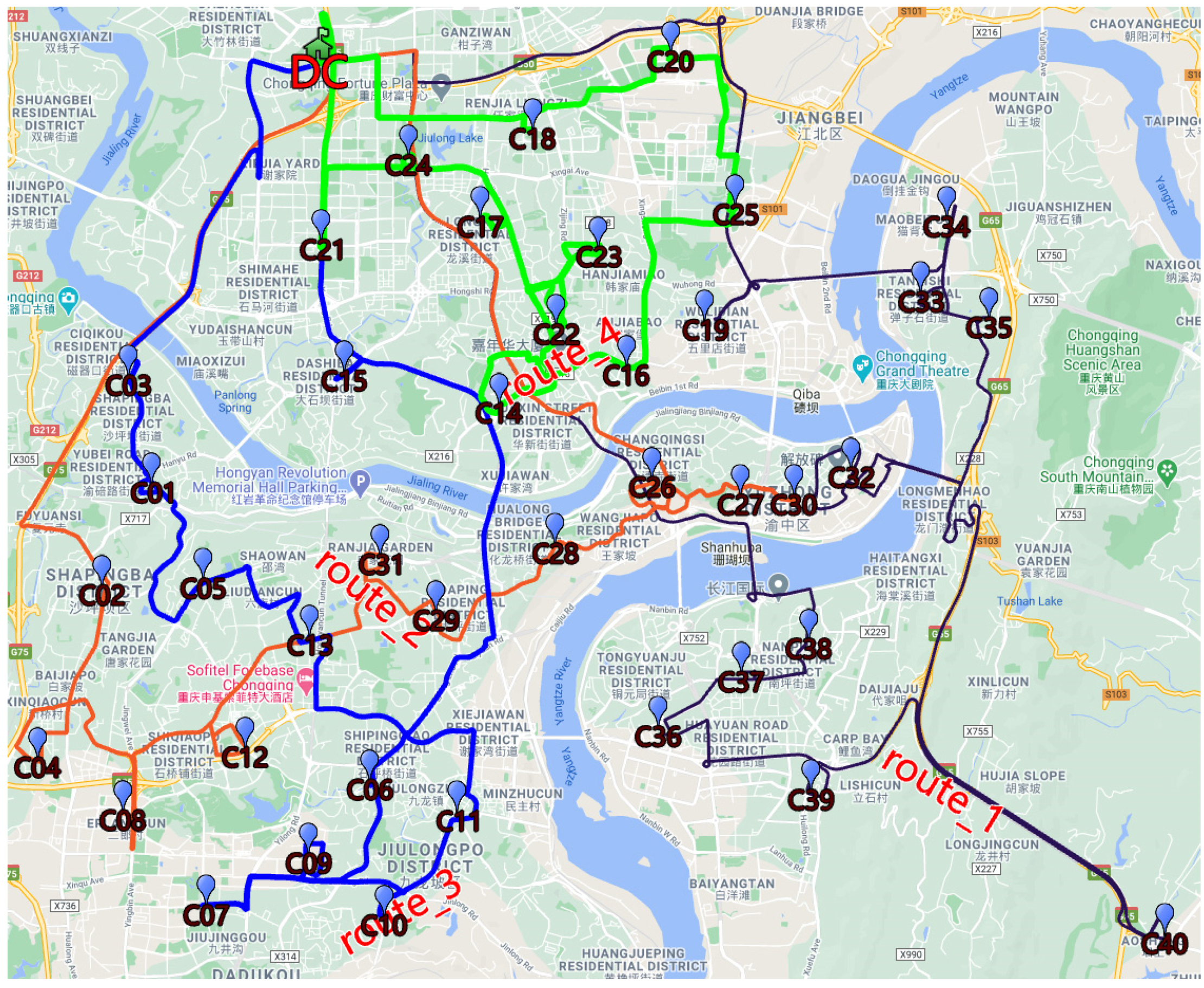
The benchmark instances tested above belong to the small-scale instance. Then, we select the instances with 100, 200, 500, 1000 and 1500 customers, respectively, (in short, JD ***, and *** represents the number of customers) from Jingdong’s delivery case in Beijing, China, as testing instances to verify the feasibility of the algorithm. The customers of the case are distributed in the Sixth Ring Road of Beijing, and the depot is located in Fangshan district of Beijing. The Haversine formula [46] is employed to calculate the distance $d_{ij}$, and the testing results are reported in

Table 4. Performance test on large-scale instances.

Instance	Vehicles	Distance (km)	Cost (CNY)
JD100	3	457.56	1815.12
JD200	8	823.6	4047.2
JD500	58	3826.63	25,053.26
JD1000	105	7195.42	45,890.84
JD1300	141	8569.18	59,438.36
JD1500	173	10,468.71	72,837.42

.

The results in Table 4 show that the proposed multi-stage heuristic algorithm is capable of solving large-scale instances.

Table 5. The time consumption of different stages.

Instance	CW (s)	TS (s)	CTO (s)	Total (s)
JD100	0.25	2.0781	0.0156	2.3
JD200	0.8438	2.4375	0.0313	3.3
JD500	2.9531	2.0313	0.0156	5
JD1000	21.9688	3.4844	0.0156	25.5
JD1300	57.4375	5.1563	0.0938	62.7
JD1500	85.3906	6.5781	0.0938	92.1

presents the CPU time of the three stages based on the large-scale instances above.

As can be seen from Table 5, the savings method in the first stage occupies most of the time in testing when the number of customers exceeds 500. Meanwhile, the time consumption of the modified tabu search algorithm in the second stage is only slightly increased with the scale, and the time consumption of the CTO algorithm in the third stage is almost negligible.

7. Case Study

The multi-stage heuristic algorithm proposed in Section 5 is used to plan freight distribution of a large supermarket in Chongqing, southwest of China. The supermarket has 40 stores (referred to as customers in what follows, numbered C01–C40) in urban areas and a large comprehensive distribution center (referred to as DC in what follows) located in the northwest of Chongqing city. The DC is responsible for the supply of certain consumer goods. The goods need to be delivered from the DC to each customer every day. The demand of customers is known in advance; thus, the demand is sent to DC every night. Then, the DC assigns deliver vehicles to meet the demand on the next day. The geographical locations of customers and DC are shown in Figure 7.

7.1. Appling the Algorithm Based on Model 1

A giant TSP tour is obtained by the savings method introduced in Section 5.1. Then, the modified tabu search algorithm proposed in Section 5.2 is performed on the giant TSP tour, which can generate an optimized giant TSP tour, and the optimized tour is divided into several routes according to the capacity constraints. Finally, an initial solution is achieved. The initial delivery routes are shown in Figure 8 and the corresponding travel distances and costs are reported in

Table 6. Comparison of travel distances and costs based on Figure 8.

	Tour Plan		Revised Tour Plan
	Distance (km)	Cost (CNY)	Distance (km)	Cost (CNY)
route_1	77.64	455.28	75.75	451.5
route_2	74.56	449.11	53.6	407.2
route_3	60.06	420.12	53.88	407.77
route_4	48.12	396.23	40.68	381.36
	260.38	1720.75	223.91	1647.83

. The tour plan on the left of Figure 8 is outputted by the modified tabu search algorithm and the revised tour plan on the right of Figure 8 is obtained by the CTO algorithm.

As shown on the right side of Figure 8, apart from the node sequence of route_3, which is not optimal, the other three routes are close to optimal. The data reported in Table 6 indicate that the CTO algorithm can reduce the total distance by 14% (36.47 km in total) and save costs by 4.24% (72.92 CNY).

After obtaining the revised tour plan, a simulation method is designed to explore the impact of different departure times on total estimated time of arrival (ETA) and emission, and even determine the best departure time. The method simulates vehicles operating their tasks by using multithreading. The calculation method of time-dependent arc durations is used to provide the time-dependent parameters based on Baidu Map APIs. The departure time starts at 6:30 a.m. and ends at 18:30 p.m. on a workday, with an interval of 1 h. The obtained results are listed in

Table 7. Simulation of the distribution process at different departure times.

Departure Time	ETA (min.)	Distance (km)	Emission (kg)
6:30	484.60	229.48	81.27
7:30	715.60	244.99	110.92
8:30	790.30	232.05	117.91
9:30	660.10	230.75	103.01
10:30	601.70	237.50	96.64
11:30	547.50	232.83	89.40
12:30	510.50	231.32	84.70
13:30	566.30	235.14	92.10
14:30	619.90	237.20	98.91
15:30	606.20	229.21	96.50
16:30	661.50	237.35	103.89
17:30	922.50	232.71	133.01
18:30	873.00	235.20	127.77
Average	658.44	234.29	102.77

.

As can be seen from Table 7, only subtle changes have been shown in terms of the total travel distance; however, selecting different departure times has a significant impact on the total ETA and emission. Because the daily replenishment of each store is not urgent, off-peak distribution may be the best way to reduce travel time and emissions. Although departing at 6.30 a.m. can completely avoid rush hour, many stores are not ready to receive their goods. Thus, a reasonable departure time is at 12:30.

The vehicle used in the case study has a self-weight of 2.8 metric tons and a maximum load of 2.5 metric tons, belonging to the diesel heavy-duty vehicle defined by the COPERT model. Therefore, the speed-dependent regression function for calculating carbon emissions is reported in

Table 8. Speed dependency of fuel consumption factors.

Speed Range (km·h−1)	Fuel Consumption Factor (g·km−1)	r2
0–47	$\mathrm{f}\left(v\right)=1425.2v^{-0.7593}$	0.99
47–100	$\mathrm{f}\left(v\right)=0.0082v^2-0.043v+60.12$	0.798

.

The variable v is the speed associated with the corresponding arc length divided by ETA obtained by the method presented in Section 3.2. The optimal speed is observed in Figure 9 according to the two speed-dependent regression functions.

As is shown in Figure 9, the piecewise function reaches the minimum value if v = 47. In other words, 47 km·h⁻¹ is the most cost-effective and eco-friendly speed. In fact, a low fuel consumption rate is presented if the speed is greater than 15 km·h⁻¹. The last column “r²” in Table 8 represents the determination coefficient of regression results. The closer the coefficient is to 1, the better the regression results are. The worst coefficient 0.798 is reported in the last row, which may be due to the insufficient number of samples with a speed greater than 47 km·h⁻¹.

The simulation method can save the cost for logistics enterprises compared with the real test of distribution process. Therefore, it can detect the best departure time for reducing the time consumption and emission.

7.2. Dynamic Route Updating Strategy

After obtaining the best departure time, a simple and fast dynamic route updating strategy is designed developed to tackle the changeable road-traffic conditions during the distribution process. The strategy starts multiple threads at run time, and the number of threads is the same as the number of routs. Each thread guides a remote vehicle and records the detailed path. If the vehicle reaches a customer node along the assigned route, the corresponding threading requests the latest distance matrix and time-dependent arc durations from Baidu Map by using the coordinates of the customer and unserved customers. Then, the OR-Tools solver is employed for solving a TSP. The next customer to be visit is determined according to the output of the solver. Finally, the real-time ETA and detailed driving paths between the two node pairs can be requested from online maps. This information is sent to the remote vehicle and recorded in a log file simultaneously.

The dynamic route updating strategy has been implemented by multithreading technology in Python [47]. Combined with the route fitting technology, the four routes are integrated into a map file shown in Figure 10 based on Google Map in an electronic view.

Using onboard global positioning system devices and communication networks, logistics companies can grasp the real-time location of delivery vehicles on electronic maps. The designed dynamic route updating procedure can be used to perceive real-time road traffic and determine the next driving path. Then, the detailed path information is transmitted to remote vehicles over the communication network.

7.3. Comparisons of Distance and Cost under Different Distance Calculation Methods

The Euclidean distance or Manhattan distance are usually adopted to calculate the distance matrix d in classic CVRP model. In fact, the alternative method of calculating the distance between each pair of points is the Haversine formula, called the Haversine distance. These distance measures can be feasible in the plain area. However, it may not work well in mountainous cities such as Chongqing, in the southwest of China, because there is a large deviation between the actual driving distance and calculated distance. To verify the impact of the different distance calculation methods, this paper conducts experiments based on the case of mountainous Chongqing City, and the result of 10 times run is presented in

Table 9. Comparison in the two methods of distance calculation.

Run No.	Real Distance		Haversine Distance
	Distance (km)	Cost (CNY)	Distance (km)	Cost (CNY)
1	238.73	1677.46	141.12	1482.24
2	248.49	1696.98	135.74	1471.48
3	230.16	1660.32	138.69	1477.38
4	227.69	1655.38	138.91	1477.82
5	242.71	1685.42	137.69	1475.38
6	239.23	1678.46	142.57	1485.14
7	237.36	1674.72	141.33	1482.66
8	235.81	1671.62	136.88	1473.76
9	248.65	1697.3	138.69	1477.38
10	244.22	1688.44	144.2	1488.4
Average	238.76	1677.52	139.07	1478.14
Radio	1.72	1.13

.

Table 9 shows that the ratio between the average actual driving distance and the Haversine distance is 1.72, whereas its cost ratio is 1.13. That is, the actual driving distance between each pair of nodes is much larger than the Haversine distance in the mountain city. Moreover, although the average distance increased by 72%, the total cost only increased by 13%. Similarly, the experiments are also performed on Jingdong instances in Beijing, China, which is a flat area. The average results are reported in

Table 10. Comparison of travel distances on large-scale instances.

Instance	Haversine Distance (km)	Real Distance (km)	R/H
JD100	457.56	738.37	1.61
JD200	823.60	1336.33	1.62
JD500	3826.63	5912.22	1.55
JD1000	7195.42	11,404.81	1.59
JD1300	8569.18	13,279.15	1.55
JD1500	10,468.71	15,997.52	1.53
Average			1.57

.

As can be seen from Table 10, the mean value of the ratio between the real driving distance and the Haversine distance (R/H) is 1.57, which is less than Chongqing’s 1.72. These ratios can provide a reference for other applications that need to estimate the actual driving distance.

The process for solving this case using the objective z₂ is similar to the above method and is not presented separately in this paper. Solving the case by considering both objectives is shown in the next section.

7.4. The Case Study Considering Both the Objective z₁ and z₂

For the data consistency and the reproducibility of experimental results, the time-dependent data used in Section 7.1 is also utilized here. Then, the algorithm is run 10 times with minimizing z₂ and the results are reported in

Table 11. The results based on minimizing z₂.

Run NO.	Distance (km)	Emission (kg)	Cost (CNY)	ETA (min.)
1	257.68	94.87	1715.35	552.19
2	231.75	92.77	1663.49	558.83
3	237.66	91.51	1675.32	541.04
4	235.19	89.74	1670.37	530.39
5	244.23	94.14	1688.46	556.82
6	240.69	93.86	1681.38	562.03
7	243.30	94.49	1686.60	563.60
8	236.13	90.03	1672.27	533.30
9	252.40	96.97	1704.80	571.44
10	256.62	95.84	1713.24	563.49
Average	243.56	93.42	1687.13	553.31

.

As can be seen from Table 11, the best solution is obtained in the fourth run, with the shortest distance of 235.19 km and the least emissions of 89.74 kg. Therefore, we can set the objective of minimizing z₁ by adding the new constraint $f_2\left(x\right)\le 89.74(1+\lambda )$ to the problem.

In this paper, the value of λ decreases from 1 to 0 with interval 0.1. The comparison between the result and the optimal solution with minimizing z₂ is reported in

Table 12. The result based on MDP.

	Distance (km)	Emission (kg)	Cost (CNY)	ETA (min.)
A satisfied solution	233.77	91.63	1667.53	543.80
The best solution with minimizing z2	235.19	89.74	1670.37	530.39

.

If the decision makers need to obtain solutions with higher quality, they just need to reduce the interval of descent and/or increase the upper bound of the counter if there is no feasible solution output, which, however, may require considerable computation time.

7.5. Managerial Insights

With the rapid increase in urban population, the number of private cars, buses, taxis and online ride-hailing vehicles has soared, resulting in frequent traffic jams. In recent years, the rapid development of e-commerce platforms has led to the increase in demand for logistics services. In the urban environment, how to deliver goods to customers in a low-cost and efficient way is the goal that decision makers of logistics pay attention to. Using the vehicle routing problem model to minimize travel distance, heuristic algorithm, simulation method of distribution scheme and dynamic route updating strategy can reduce the distribution cost of enterprises and improve their revenues. On the contrary, how to reduce the impact of delivery vehicles on the urban environment is the goal of governmental managers. The carbon emissions of distribution vehicles can be reduced by using the vehicle routing problem model with minimization carbon emissions, algorithm and the above two additional methods. The bi-objective model considering the minimization of travel distance and carbon emissions is very suitable in the context of energy saving and carbon reduction. No matter the single-objective model or the bi-objective model, the influence of traffic congestion on the model parameters should be considered in urban distribution scenarios. The calculation method of time-dependent arc durations can be used by the decision makers of logistics enterprises to estimate the time-dependent parameters in the distribution process. Combining the simulation method and dynamic route updating strategy ensures that the distribution tasks can be successfully completed in the road network of the target region. In addition, based on the online route update strategy, decision makers of logistics enterprises can use the free transport capacity resources to respond to the dynamic requests of customers quickly, and then obtain more income with lower route costs and carbon emissions. Finally, if the actual driving distance between node pairs is hard to collect, the decision makers of logistics enterprises can calculate an arc distance using the Haversine formula, and then the actual driving distance is estimated by multiplying the arc distance times the road detour coefficient (R/H) of the target area.

8. Conclusions and Future Work

This paper designs a multi-stage heuristic algorithm for the proposed CVRP models. The algorithm simplifies the savings method, adds four neighborhood operators into the tabu search algorithm to increase its diversity and enhances the solution quality by using the CTO algorithm. The accuracy and feasibility of the algorithm are verified by dealing with the benchmark instances and real large-scale instances. In addition, the daily distribution case of the supermarket shows that the designed algorithm can gradually improve the solution quality and finally obtain a good distribution scheme. The routes servicing all customers are vividly displayed in the real road network by means of the post-processing procedures. As for the bi-objective model, the modified framework is developed by using the multi-objective decision making method with relaxation coefficient. Decision-makers can flexibly set the relaxation coefficient according to their real needs to obtain the corresponding solutions.

Although the models and solution approach have many features, there are still some limitations in this study. The designed multi-stage heuristic algorithm abandons a lot of local search procedures in the third stage to achieve faster solution speed; therefore, it could be a good choice to apply some intra-route or inter-route node-exchange/relocation operators without greatly increasing computation time. Additionally, it could be significantly meaningful to further investigate the relationships between departure time, travel duration, travel distance and emissions. Moreover, because the splitting method for the giant TSP tour is linear, more effective methods could be developed.

References

1. Hannan, M.A.; Begum, R.; Al-Shetwi, A.Q.; Ker, P.; Al Mamun, M.; Hussain, A.; Basri, H.; Mahlia, T. Waste collection route optimisation model for linking cost saving and emission reduction to achieve sustainable development goals. Sustain. Cities Soc. 2020, 62, 102393. [Google Scholar] [CrossRef]
2. Letchford, A.N.; Lysgaard, J.; Eglese, R.W. A branch-and-cut algorithm for the capacitated open vehicle routing problem. J. Oper. Res. Soc. 2007, 58, 1642–1651. [Google Scholar] [CrossRef]
3. Christiansen, C.H.; Lysgaard, J. A branch-and-price algorithm for the capacitated vehicle routing problem with stochastic demands. Oper. Res. Lett. 2007, 35, 773–781. [Google Scholar] [CrossRef]
4. Xie, Y.; Lu, W.; Wang, W.; Quadrifoglio, L. A multimodal location and routing model for hazardous materials transportation. J. Hazard. Mater. 2012, 227–228, 135–141. [Google Scholar] [CrossRef]
5. Gauvin, C.; Desaulniers, G.; Gendreau, M. A branch-cut-and-price algorithm for the vehicle routing problem with stochastic demands. Comput. Oper. Res. 2014, 50, 141–153. [Google Scholar] [CrossRef]
6. Santos, F.A.; Mateus, G.R.; da Cunha, A.S. A Branch-and-Cut-and-Price Algorithm for the Two-Echelon Capacitated Vehicle Routing Problem. Transp. Sci. 2015, 49, 355–368. [Google Scholar] [CrossRef]
7. Dinh, T.; Fukasawa, R.; Luedtke, J. Exact algorithms for the chance-constrained vehicle routing problem. Math. Program. 2017, 172, 105–138. [Google Scholar] [CrossRef]
8. Munari, P.; Moreno, A.; De La Vega, J.; Alem, D.; Gondzio, J.; Morabito, R. The Robust Vehicle Routing Problem with Time Windows: Compact Formulation and Branch-Price-and-Cut Method. Transp. Sci. 2019, 53, 1043–1066. [Google Scholar] [CrossRef]
9. Florio, A.M.; Hartl, R.F.; Minner, S. New Exact Algorithm for the Vehicle Routing Problem with Stochastic Demands. Transp. Sci. 2020, 54, 1073–1090. [Google Scholar] [CrossRef]
10. Xiao, Y.; Zuo, X.; Huang, J.; Konak, A.; Xu, Y. The continuous pollution routing problem. Appl. Math. Comput. 2020, 387, 125072. [Google Scholar] [CrossRef]
11. Zhang, L.; Liu, Z.; Yu, L.; Fang, K.; Yao, B.; Yu, B. Routing optimization of shared autonomous electric vehicles under uncertain travel time and uncertain service time. Transp. Res. Part E Logist. Transp. Rev. 2021, 157, 102548. [Google Scholar] [CrossRef]
12. Clarke, G.; Wright, J.W. Scheduling of Vehicles from a Central Depot to a Number of Delivery Points. Oper. Res. 1964, 12, 568–581. [Google Scholar] [CrossRef]
13. Zidi, I.; Al-Omani, M.; Aldhafeeri, K. A New Approach Based on the Hybridization of Simulated Annealing Algorithm and Tabu Search to Solve the Static Ambulance Routing Problem. Procedia Comput. Sci. 2019, 159, 1216–1228. [Google Scholar] [CrossRef]
14. Omidvar, A.; Ozguven, E.E.; Vanli, O.A.; Tavakkoli-Moghaddam, R. A two-phase safe vehicle routing and scheduling problem: Formulations and solution algorithms. Arxiv Prepr. 2017, arXiv:07147. [Google Scholar]
15. Marinakis, Y.; Marinaki, M.; Dounias, G. A hybrid particle swarm optimization algorithm for the vehicle routing problem. Eng. Appl. Artif. Intell. 2010, 23, 463–472. [Google Scholar] [CrossRef]
16. Rong, L.; Xu, M. Impact of Altruistic Preference and Government Subsidy on the Multinational Green Supply Chain under Dynamic Tariff. Environ. Dev. Sustain. 2021, 24, 1928–1958. [Google Scholar] [CrossRef]
17. Akeb, H.; Bouchakhchoukha, A.; Hifi, M. A Three-Stage Heuristic for the Capacitated Vehicle Routing Problem with Time Windows, in Recent Advances in Computational Optimization: Results of the Workshop on Computational Optimization WCO 2013; Fidanova, S., Ed.; Springer International Publishing: Cham, Cambodia, 2015; pp. 1–19. [Google Scholar]
18. Ichoua, S.; Gendreau, M.; Potvin, J.-Y. Vehicle dispatching with time-dependent travel times. Eur. J. Oper. Res. 2003, 144, 379–396. [Google Scholar] [CrossRef]
19. Lecluyse, C.; Van Woensel, T.; Peremans, H. Vehicle routing with stochastic time-dependent travel times. 4OR A Q. J. Oper. Res. 2009, 7, 363–377. [Google Scholar] [CrossRef]
20. Jabali, O.; Van Woensel, T.; de Kok, A.G. Analysis of Travel Times and CO2Emissions in Time-Dependent Vehicle Routing. Prod. Oper. Manag. 2012, 21, 1060–1074. [Google Scholar] [CrossRef]
21. Qian, J.; Eglese, R. Fuel emissions optimization in vehicle routing problems with time-varying speeds. Eur. J. Oper. Res. 2016, 248, 840–848. [Google Scholar] [CrossRef]
22. Çimen, M.; Soysal, M. Time-dependent green vehicle routing problem with stochastic vehicle speeds: An approximate dynamic programming algorithm. Transp. Res. Part D Transp. Environ. 2017, 54, 82–98. [Google Scholar] [CrossRef]
23. Wang, Y.; Assogba, K.; Fan, J.; Xu, M.; Liu, Y.; Wang, H. Multi-depot green vehicle routing problem with shared transportation resource: Integration of time-dependent speed and piecewise penalty cost. J. Clean. Prod. 2019, 232, 12–29. [Google Scholar] [CrossRef]
24. Huang, Y.; Zhao, L.; Van Woensel, T.; Gross, J.-P. Time-dependent vehicle routing problem with path flexibility. Transp. Res. Part B Methodol. 2017, 95, 169–195. [Google Scholar] [CrossRef]
25. Ma, Z.-J.; Wu, Y.; Dai, Y. A combined order selection and time-dependent vehicle routing problem with time widows for perishable product delivery. Comput. Ind. Eng. 2017, 114, 101–113. [Google Scholar] [CrossRef]
26. Fan, H.; Zhang, Y.; Tian, P.; Lv, Y.; Fan, H. Time-dependent multi-depot green vehicle routing problem with time windows considering temporal-spatial distance. Comput. Oper. Res. 2021, 129, 105211. [Google Scholar] [CrossRef]
27. Allahyari, S.; Yaghoubi, S.; Van Woensel, T. The secure time-dependent vehicle routing problem with uncertain demands. Comput. Oper. Res. 2021, 131, 105253. [Google Scholar] [CrossRef]
28. Schmidt, C.E.; Silva, A.C.; Darvish, M.; Coelho, L.C. Time-dependent fleet size and mix multi-depot vehicle routing problem. Int. J. Prod. Econ. 2023, 255, 108653. [Google Scholar] [CrossRef]
29. Costa, L.; Lust, T.; Kramer, R.; Subramanian, A. A two-phase Pareto local search heuristic for the bi-objective pollution-routing problem. Networks 2018, 72, 311–336. [Google Scholar] [CrossRef]
30. Poonthalir, G.; Nadarajan, R. A Fuel Efficient Green Vehicle Routing Problem with varying speed constraint (F-GVRP). Expert Syst. Appl. 2018, 100, 131–144. [Google Scholar] [CrossRef]
31. Zhao, P.; Luo, W.; Han, X. Time-dependent and bi-objective vehicle routing problem with time windows. Adv. Prod. Eng. Manag. 2019, 14, 201–212. [Google Scholar] [CrossRef]
32. Zhou, J.; Zhang, M.; Wu, S. Multi-Objective Vehicle Routing Problem for Waste Classification and Collection with Sustainable Concerns: The Case of Shanghai City. Sustainability 2022, 14, 11498. [Google Scholar] [CrossRef]
33. Ghannadpour, S.F.; Zarrabi, A. Multi-objective heterogeneous vehicle routing and scheduling problem with energy minimizing. Swarm Evol. Comput. 2018, 44, 728–747. [Google Scholar] [CrossRef]
34. Ren, X.; Huang, H.; Feng, S.; Liang, G. An improved variable neighborhood search for bi-objective mixed-energy fleet vehicle routing problem. J. Clean. Prod. 2020, 275, 124155. [Google Scholar] [CrossRef]
35. Islam, A.; Gajpal, Y.; ElMekkawy, T.Y. Mixed fleet based green clustered logistics problem under carbon emission cap. Sustain. Cities Soc. 2021, 72, 103074. [Google Scholar] [CrossRef]
36. Amiri, A.; Amin, S.H.; Zolfagharinia, H. A bi-objective green vehicle routing problem with a mixed fleet of conventional and electric trucks: Considering charging power and density of stations. Expert Syst. Appl. 2023, 213, 119228. [Google Scholar] [CrossRef]
37. Glize, E.; Jozefowiez, N.; Ngueveu, S.U. An ε-constraint column generation-and-enumeration algorithm for Bi-Objective Vehicle Routing Problems. Comput. Oper. Res. 2022, 138, 105570. [Google Scholar] [CrossRef]
38. Zarouk, Y.; Mahdavi, I.; Rezaeian, J.; Santos-Arteaga, F.J. A novel multi-objective green vehicle routing and scheduling model with stochastic demand, supply, and variable travel times. Comput. Oper. Res. 2022, 141, 105698. [Google Scholar] [CrossRef]
39. EMISIA. Methodology for the Calculation of Emissions–COPERTE V. 2022. Available online: https://www.emisia.com/utilities/copert/documentation/ (accessed on 3 November 2022).
40. Ntziachristos, L.; Samaras, Z. Copert III Methodology and Emission Factors (Version 2.1); Eggleston, S., Gorissen, N., Hassel, D., Hickman, A.-J., Joumard, R., Rijkeboer, R., White, L., Zierock, K.-H., Eds.; European Environment Agency, ETC/AE: Copenhagen, Denmark, 2000; Available online: https://vergina.eng.auth.gr/mech/lat/copert/C3v2_1MR.pdf (accessed on 1 May 2022).
41. Gendreau, M. An Introduction to Tabu Search. In Handbook of Metaheuristics; Glover, F., Kochenberger, G.A., Eds.; Springer US: Boston, MA, USA, 2003; pp. 37–54. [Google Scholar]
42. Jin, Y.; Ge, X.; Zhang, L.; Ren, J. A two-stage algorithm for bi-objective logistics model of cash-in-transit vehicle routing problems with economic and environmental optimization based on real-time traffic data. J. Ind. Inf. Integr. 2021, 26, 100273. [Google Scholar] [CrossRef]
43. Bondy, J.A.; Murty, U.S.R. Graph Theory, 1st ed.; Springer: Berlin/Heidelberg, Germany, 2007; p. 650. [Google Scholar]
44. Augerat, P.; Naddef, D.; Belenguer, J.M.; Benavent, E.; Corberan, A.; Rinaldi, G. The VRP Web. 2022. Available online: http://www.bernabe.dorronsoro.es/vrp/index.html (accessed on 3 March 2022).
45. Jingdong (JD). The Global Optimization Challenge. 2018. Available online: https://medium.com/jd-technology-blog (accessed on 3 March 2022).
46. Nichat, M.K.; Chopde, R.N.; Nichat, M. Landmark Based Shortest Path Detection By Using A* Algorithm and Haversine Formula. Int. J. Innov. Res. Comput. Commun. Eng. 2013, 1, 299. [Google Scholar]
47. Ge, X.; Jin, Y.; Zhang, L. Genetic-based algorithms for cash-in-transit multi depot vehicle routing problems: Economic and environmental optimization. Environ. Dev. Sustain. 2022, 25, 557–586. [Google Scholar] [CrossRef]
Figure 1. The detailed information of calculating the time-dependent arc durations.
Sustainability 15 03208 g001
Figure 2. The framework of multi-stage heuristic algorithm.
Sustainability 15 03208 g002
Figure 3. An illustration of the savings method.
Sustainability 15 03208 g003
Figure 4. An illustration of neighborhood operators.
Sustainability 15 03208 g004
Figure 5. An illustration of the CTO algorithm.
Sustainability 15 03208 g005
Figure 6. The modified solution framework for bi-objective models.
Sustainability 15 03208 g006
Figure 7. The geographical location of nodes.
Sustainability 15 03208 g007
Figure 8. Comparison of the results obtained by the last two stages of the proposed algorithm.
Sustainability 15 03208 g008
Figure 9. The relationship between speeds and fuel consumption factors.
Sustainability 15 03208 g009
Figure 10. Real distribution routes.
Sustainability 15 03208 g010