The Spatio-Temporal Pattern of Regional Coordinated Development in the Common Prosperity Demonstration Zone—Evidence from Zhejiang Province

Abstract

Achieving common prosperity is the essential requirement of socialism and promoting regional coordinated development (RCD) is an important path to achieving common prosperity. This study uses data from Zhejiang Province from 2011 to 2020, a demonstration zone of common prosperity, to construct an evaluation model of RCD, assess the regional development level and coordinated development degree, and then analyze the regional differences and spatial correlation pattern of RCD. The following results were obtained: (1) The economic, social, and ecological subsystems of all cities or counties show a continuous or fluctuating rise, and the regional coordinated development level of each study unit also shows a rising trend. This shows that steady regional development is the fundamental material basis for common prosperity. (2) The level of economic and social development shows a pattern of high in the north and low in the south, while the level of ecological development shows a pattern of high in the south and low in the north. The level of RCD evolves from a very uneven spatial distribution to a good level of coordinated development in most cities. It shows that the equalization of development among regions is a realistic manifestation of common prosperity. (3) The level of RCD in Zhejiang Province has greater intra-regional than inter-regional differences, and the differences in RCD in the north are greater than those in the south. The differences between regions have been narrowing. It shows a significant positive spatial correlation, with high-value regions tending to be adjacent to high-value regions and low-value regions tending to be adjacent to low-value regions. In sum, the development of Zhejiang Province in the last decade provides evidence of its role as a demonstration zone for common prosperity. It confirms that coordinated regional development is the fundamental way to achieve common prosperity.

1. Introduction

Common prosperity is the essential provision of socialism with Chinese characteristics and the goal of China’s struggle at this stage [1]. In 2020, the Communist Party of China (CPC) has made a major strategic plan to “solidly promote common prosperity”. In 2021, the 14th Five-Year Plan and the outline of the 2035 Vision put forward the requirement of promoting common prosperity and supported Zhejiang’s high-quality development to build a common prosperity demonstration zone. In 2022, the 20th National Congress of CPC first proposed that common prosperity is an important feature of Chinese-style modernization. In the latest theory of Marxism’s Chineseization, regional coordinated development (RCD) is a major initiative to promote common prosperity [2]. Unbalanced and insufficient regional development is a constraint to solidly promoting common prosperity, which must be achieved with RCD. The important thesis of RCD in the new era sprouted from the “Mountain and Sea Collaboration Project” introduced by Zhejiang Province in 2003, which is an important initiative to promote common prosperity [3]. The 18th National Congress pointed out that “promoting coordinated development, synergistic and common development in all regions”, the 19th National Congress pointed out that the “overall strategy for regional development” has been upgraded to a “regional coordinated development strategy”, and the 20th National Congress placed “coordination” in the prominent position of regional development. Therefore, this study measures and evaluates various aspects of Zhejiang Province under the perspective of common prosperity with the level of RCD as the criterion and suggests development policies for other provinces.

In 2020, China’s per capita GDP reached USD 11,300, per capita disposable income reached USD 32,189, and its urbanization rate reached 63.89%. The development of the national economy and cities has made high achievements, but unbalanced and insufficient development is still the main problem of Chinese society. As a demonstration zone for common prosperity, Zhejiang Province has the following two advantages [4]: (1) A high degree of prosperity, per capita disposable income of CNY 52,397 in 2020, only lower than Beijing and Shanghai, a per capita GDP of CNY 101,000, ranking sixth in the country, and urban and rural residents’ income for 20 and 36 consecutive years, respectively, ranked no. 1 in the country’s provinces and regions. (2) A high degree of common, the income ratio of urban and rural residents in 2020 was 1.96:1. It was only higher than Tianjin and Heilongjiang, whose income ratio of urban and rural residents in 2020 was 1.67:1. It is the only province in which the income of residents of all municipalities exceeds the national average. Therefore, Zhejiang Province has served as a demonstration zone for common prosperity. The following issues are studied using spatial-temporal analysis from the three subsystems of economy, society, and ecology under the system of RCD: (1) To assess the governance effects of coordinated regional development. (2) To summarize the governance experience of coordinated regional development as well as its optimization and improvement.

The system of measurement indicators focuses on two aspects—coordination and development. Qin (2013) constructs the evaluation system of the regional economic coordinated development level from inter-regional economic linkage, regional economic growth, and the regional economic difference value [5]. Yang (2017) constructs the evaluation system of coordinated development from urbanization, informatization, industrialization, greening, and agricultural modernization [6]. Ruan (2017) constructs the degree of coordinated urban–rural development from the development indexes of urban and rural areas [7]. Deng (2019) measures the coordinated development of the region from the coordination of the development of three major economic, social, and ecological systems [8]. The model of the common prosperity index is constructed from three aspects of development, sharing, and sustainability [9]. In the process of index construction, the related literature neglects the mutual influence relationships among the indexes, resulting in the redundancy of the indexes, and the weight determination process is too subjective, or the amount of data is insufficient, resulting in a reduction in the validity of the weights. Therefore, this paper improves the index system setting and weight calculation methods, which are described in Section 2.1 Indicator System.

This paper focuses on measuring and analyzing the development level, coordination degree, regional differences, and spatial correlation pattern of the RCD. The measurements in the references are organized according to the above four aspects. (1) The measurement of development level is mainly evaluated and measured using the entropy-weighted TOPSIS model [10], quadratic weighted principal component analysis [11], and AHP-fuzzy comprehensive evaluation method [12]. (2) For the measurement of the coordination level, some scholars in the existing research construct the formula for the coordination coefficient among population, land, and economic systems and grade the level of coordinated development [13]. (3) For the analysis of regional differences, some scholars decompose and study the level of water resources [14], employment segregation [15], land use efficiency [16], and green technology innovation efficiency [17] using the Theil index. (4) The spatial correlation pattern is mainly measured using the Moran index [18].

Based on the literature, RCD is the coordinated and sustainable development among economic, social, and ecological subsystems within a region on the one hand, and the coordinated economic development between regions on the other [19]. This study argues that while ensuring the coordinated development of subsystems within a region, it is also necessary to reduce the differences in coordinated development between regions and gradually achieve common prosperity under the joint promotion of the market and government. Therefore, the level of RCD needs to be measured in four aspects: development level, degree of coordination, regional differences, and spatial correlation pattern. The main contribution of this study is to provide empirical evidence for the socialist theory of commonwealth with Chinese characteristics in practice [20] and to further analyze the spatial and temporal pattern of regional coordinated development in Zhejiang Province at the county scale in a more microscopic and detailed way, and its practical experience can also provide a reference for other regions.

The remainder of this paper is organized as follows. Section 2 presents the main indicators, data sources, and study area of this paper. Section 3 presents the main methods, such as the PCA-TOPSIS model, the Coordinated Development Model, and the Theil and Moran indices, in preparation for the empirical analysis in the later section. Section 4 presents the empirical results and analysis. Section 5 provides conclusions and policy recommendations.

2. Indicator System and Data Sources

2.1. Indicator System

According to the 14th Five-Year Plan and the outline of the 2035 Vision, the national economy, social development, and ecological civilization are equally important. On the premise of data availability, following the principles of scientific, systematic, and representative, and based on the existing regional coordinated development performance measurement index system in the literature, this study identifies three major target layers including the economic, social, and ecological subsystems. A total of 19 indicators were eventually selected and distinguished between the positive and negative direction of the indicators, as shown in

Table 1. Evaluation system of indicators for measuring the level of regional coordinated development.

Target Layer	Criterion Layer	Indicator Layer	Direction	Weight
Economic Subsystem	Economic strength	Per capita GDP (CNY 10,000)	Positive	23.03
		Per capita total retail sales of consumer goods	Positive	25.55
		Per capita local fiscal revenue (CNY 10,000)	Positive	22.89
	Economic structure	The ratio of the tertiary industry to GDP (%)	Positive	3.19
		Industrial output as a ratio of industrial and agricultural industries (%)	Positive	17.04
	Economic openness	Total imports and exports (USD 10,000)	Positive	8.30
Social Subsystem	Infrastructure	Number of beds in medical institutions per 10,000 population (beds per 10,000 population)	Positive	12.83
		Mobile phone subscriptions per capita (households/person)	Positive	13.15
		Freight traffic per capita (tons/person)	Positive	6.72
	Social Security	Urban to rural income ratio (%)	Negative	3.04
		Medical insurance coverage (%)	Positive	13.50
		Pension insurance coverage (%)	Positive	9.52
		Unemployment insurance coverage (%)	Positive	13.33
	Science and Education	Education as a share of fiscal expenditure (%)	Positive	6.94
		Number of primary and secondary school students per capita (students)	Positive	11.31
		Number of invention patents per 10,000 people (pieces per 10,000 people)	Positive	9.65
Ecological Subsystem	Resource utilization	Crop area is sown per capita (thousands of hectares per 10,000 people)	Positive	26.46
	Environmental quality	Air quality PM2.5 concentration (μg/m3)	Negative	50.69
	Green development	Carbon emissions per unit of GDP (million tons/billion RMB)	Negative	22.85

. Among them, the weight is calculated with the PCA method, which is detailed in Section 3.1.2.

Firstly, six indicators are constructed to evaluate the level of development of the economic subsystem from three criterion levels: economic strength, economic structure, and economic openness. Among them, GDP, total retail consumer goods [21], and local fiscal revenue are used to measure economic strength, the ratio of the tertiary industry to GDP and industrial output as a ratio of industrial and agricultural industries are used to measure economic structure, and total imports and exports are used to measure economic openness [22].

Secondly, ten indicators are constructed to evaluate the level of development of social subsystems from three guideline layers: infrastructure, social security, and level of science and education. Among them, infrastructure is measured using the per capita value of hospital beds, mobile phones, and freight transport. Social security is measured in terms of health, pension, unemployment insurance, and the urban–rural income ratio. The level of science and education is measured using the share of education investment in fiscal revenue, as well as the number of primary and secondary school students and patents for inventions per capita.

Thirdly, three indicators are constructed to evaluate the development level of the ecological subsystem from three criteria layers of resource utilization, environmental quality, and green development. Crop area sown per capita is used to measure resource utilization, air quality PM 2.5 concentration is used to measure environmental quality, and carbon emissions per unit of GDP are used to measure green development [23].

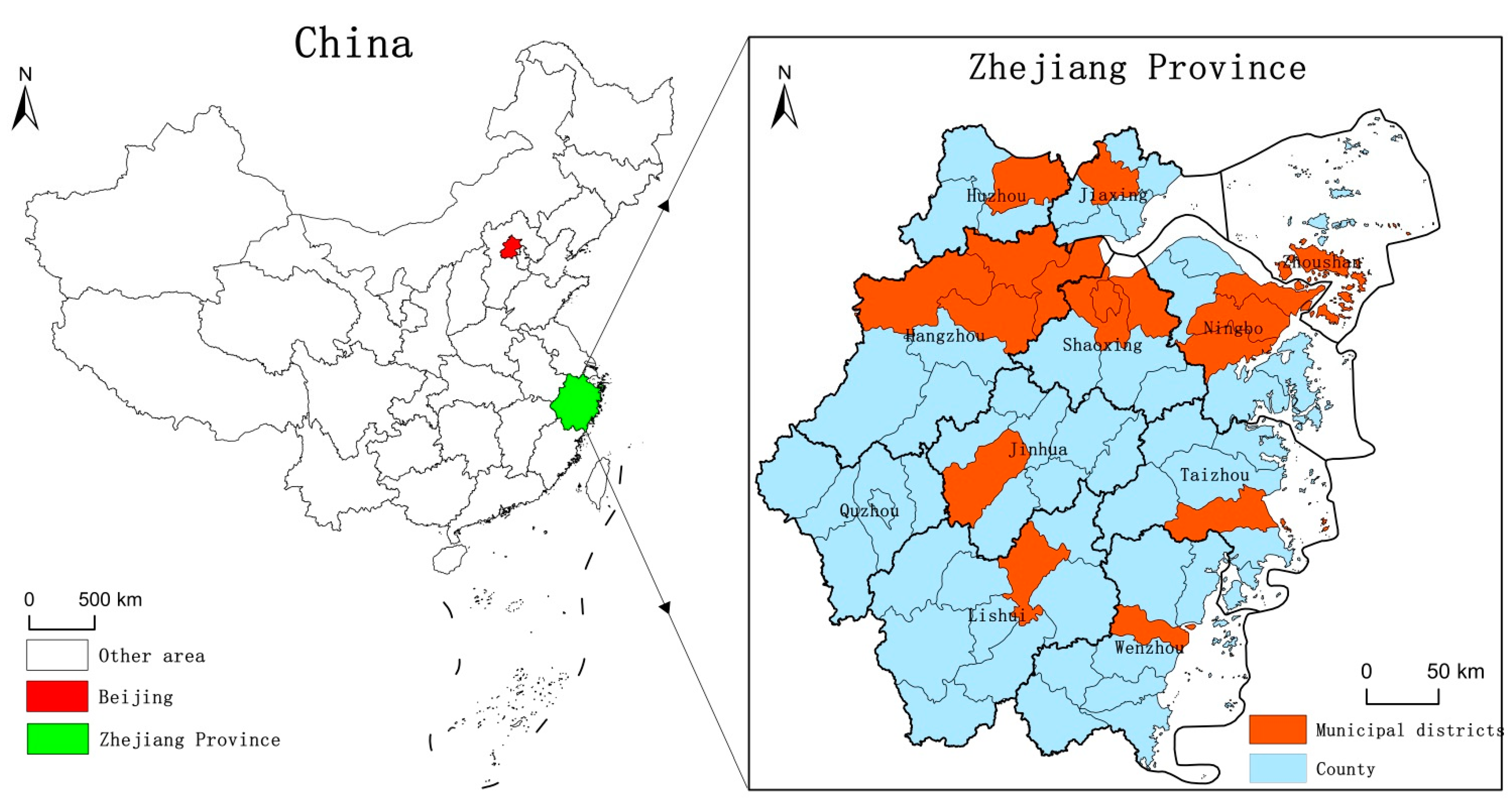
2.2. Data Sources and Study Area

Zhejiang Province is located in southeastern China and is a pioneering region for reform and opening up. Zhejiang Province has a total area of 105,500 square kilometers, 11 cities at the prefecture level, 37 municipal districts, 20 county-level cities, and 33 counties (including one autonomous county.) By 2020, the per capita disposable income of urban residents had ranked first among all provinces and regions in China for 20 consecutive years, and the per capita disposable income of rural residents had also remained first for 36 consecutive years. In 2021, the Central Committee of the Communist Party of China and the State Council supported Zhejiang’s high-quality development to build a model zone of common prosperity. By the end of 2021, Zhejiang Province had a resident population of 65.4 million and a GDP of CNY 735.16 billion. Figure 1 shows the geographical location of Zhejiang Province in China and the counties and municipal districts within the province.

This study takes 58 counties and 11 municipalities in Zhejiang Province as study units. In addition, this study selects the study period from 2011 to 2020. The economic and social data are from the Zhejiang Statistic Yearbook (2012–2021) and China Urban Statistic Yearbook (2012–2021). The carbon emission data are from the database of CEADs as the basis for green development. The air quality data are from the Atmospheric Composition Analysis Group, Dalhousie University. The missing data are complemented using the arithmetical method of linear interpolation with Stata 17 software. The data are analyzed and processed using SPSS 26, Stata 17, Microsoft Excel 2010, and Geoda. The map data are processed and generated using ArcGIS 10.6.

3. Methods

3.1. PCA-TOPSIS Model

TOPSIS is widely used in the economic, management, and social fields. The evaluation of RCD that we focus on in this paper can use this method. While the traditional TOPSIS mainly determines weights based on subjective opinions [24], such as the analytic hierarchy process (AHP method) [25], the expert scoring method [26] is more subjective, which may cause the evaluation results to be inaccurate or biased. Therefore, this study uses principal component analysis (PCA method) [27] to avoid subjective errors, so that the decision matrix of the assessment object and the determination of positive and negative ideal solutions can be improved. With these considerations, the PCA-TOPSIS model is used to measure the development level of the regional coordinated development system and its subsystems in the common prosperity demonstration zone.

3.1.1. Standardization of Initial Indicator Data

The initial matrix $R$ of evaluation subjects is defined as Equation (1), $X_{ij}$ is the indicator value of the $i$ evaluation indicator of the evaluation object in the $j$ region, where $m$ is the number of evaluation indicators and $n$ is the number of evaluation regions. Since the attributes such as units and order of magnitude are different for each participant indicator, the data are dimensionless using the extreme difference regularization method, so that $X{’}_{ij}$∈ [0, 1], resulting in a standardization matrix, $R={\left[X{\prime }_{ij}\right]}_{mn}$.

For positive indicators, the dimensionless is based on Equation (2). For negative indicators, the dimensionless is based on Equation (3). Among them, $X{\prime }_{ij}$ is the indicator value after data normalization, $X_{jmin}$ is the minimum value of indicator $j$ in all regions, and $X_{jmax}$ is the maximum value of indicator $j$ in all regions.

$$R=\left[\begin{array}{ccc}{X}_{11}& \cdots & X_{1n}\\ ⋮& \ddots & ⋮\\ X_{m1}& \cdots & X_{mn}\end{array}\right](m=1,2,3\text{...},n=1,2,3)$$

(1)

$$X{\prime }_{ij}=\left(X_{ij}-X_{jmin}\right)/\left(X_{jmax}-X_{jmin}\right)$$

(2)

$$X{\prime }_{ij}=\left(X_{jmax}-X_{ij}\right)/\left(X_{jmax}-X_{jmin}\right)$$

(3)

3.1.2. Principal Component Analysis to Determine Weights

The linear combination coefficient matrix is described in Equation (4), and the load factor $a_{ij}$ is divided by the square root of the corresponding characteristic root ${\lambda }_i$ to obtain the principal component expression coefficient $e_{ij}$. The combined score coefficient vectors are described in Equation (5), the linear combination coefficients $e_{ij}$ are multiplied by the variance interpretation rate $r_i$, respectively, and accumulated and divided by the cumulative variance interpretation rate $r_i$ to obtain the combined score coefficient vector $y_j$. Utilizing Equation (6), the combined score coefficients are normalized to obtain the weighting values for each indicator.

$$e_{ij}=a_{ij}/\sqrt{{\lambda }_i}$$

(4)

$$y_j=\frac{{{\displaystyle \sum }}_{i=1}^5{r}_i{e}_{ij}}{r_i}$$

(5)

$$w_j=\frac{y_j}{{{\displaystyle \sum }}_{j=1}^{15}{y}_j}$$

(6)

However, negative weights occur during the calculation of the weights as described above, so the negative weights in the normalization process are dealt with by shifting the axes and mapping [28]. The shifting of the axes can be defined as Equation (7), which includes shifting the origin from point 0 to point $-K$, removing the negative value, and taking $K=\underset{1\le j\le 15}{\max }\left|w_j\right|$. The mapping can be expressed as Equation (8), which includes compressing $\left(K+w_j\right)$ to the interval [0, 1]. In the above weighting measurement, the cumulative percentage of the variance of the principal components is greater than 80% and, therefore, the weighting calculation is qualified.

$$f_j=\frac{K+w_j}{2K}$$

(7)

$$w_j^{’}=\frac{f_j}{{{\displaystyle \sum }}_{j=1}^{15}{w}_j}$$

(8)

3.1.3. TOPSIS Model Development Level Measurements

Let the weighted decision evaluation matrix be $V$, as shown in the following Equation (9), where the weight vector $W$ is formed based on the indicator weights $w_j^{\prime }$, combined with the normalization matrix $P={\left[p_{ij}\right]}_{mn}$, to obtain the weighted normalization matrix $V$.

$$V=P\times W={\left[v_{ij}\right]}_{mn}$$

(9)

The positive and negative ideal solutions are defined as Equations (10) and (11), respectively, where $V^{+}$ is the positive ideal solution and $V^{-}$ is the negative ideal solution. The positive ideal solution, also known as the optimal solution, is the set of maximum values of each indicator, and the negative ideal solution, also known as the inferior solution, is the set of minimum values of each indicator.

$$V^{+}=\left\{max{V}_{ij}/i=1,2,\dots ,m\right\}=\left\{V_1^{+},V_2^{+},\dots ,V_m^{+}\right\}$$

(10)

$$V^{-}=\left\{min{V}_{ij }/i=1,2,\dots ,m\right\}=\left\{V_1^{-},V_2^{-},\dots ,V_m^{-}\right\}$$

(11)

The distances from the evaluation vectors to the identified positive and negative ideal solutions are calculated for each region using Equations (12) and (13) respectively, with $D_j^{+}$ being the distance from the evaluation vector to the positive ideal solution for each region and $D_j^{-}$ being the distance from the evaluation vector to the negative ideal solution for each region.

$$D_j^{+}=\sqrt{{{\displaystyle \sum }}_{i=1}^m{\left(V_i^{+}-V_{ij}\right)}^2}$$

(12)

$$D_j^{-}=\sqrt{{{\displaystyle \sum }}_{i=1}^m{\left(V_i^{-}-V_{ij}\right)}^2}$$

(13)

Eventually, T_j denotes the closeness of the evaluation target to the optimal solution with a value range of [0, 1], where a higher value means that the evaluation result of the subject is closer to the optimal level, meaning the more advanced the level of regional development, which is calculated using Equation (14).

$$T_j=\frac{D_j^{-}}{D_j^{+}+D_j^{-}}$$

(14)

The natural interval method [29] was used to classify the closeness into four levels indicating the level of development in the assessment target, where $\mu$ is the average value and $\mathsf{\sigma }$ is the standard deviation of closeness for each city and county in the same subsystem from 2011 to 2020. The closeness can be divided into four levels indicating the level of development in the assessment target [30] and is also used for ArcGIS mapping; the grading is shown in

Table 2. The closeness levels.

Closeness	Level
[0, $\mathsf{\mu }-\mathsf{\sigma }$]	Low
[$\mathsf{\mu }-\mathsf{\sigma }$, $\mathsf{\mu }$]	Moderate
[$\mathsf{\mu }$, $\mathsf{\mu }+\mathsf{\sigma }$]	Good
[$\mathsf{\mu }+\mathsf{\sigma }$, 1]	Excellent

.

3.2. Coordinated Development Model

To measure the coordinated development between the economy, society, and ecology, a coordinated development model is constructed regarding the relevant literature [31]. The model uses the coordinated development degree function to calculate the regional development coordination coefficient of the evaluation unit. After mathematical derivation, $C_i$ takes values in the range of [1,$\sqrt{3}$]. This study projects the coordination coefficient $C_i$ to the interval of [0, 1], meaning that $C_i^{’}=\left(C_i - 1\right)/\left(\sqrt{3}-1\right)$, resulting in the coordination degree $C_i^{\prime }$. The grading results [32] are shown in

Table 3. Coordination degree levels.

Coordination Degree	Level
[0, 0.5)	Uncoordinated
[0.5, 0.6)	Barely coordination
[0.6, 0.7)	Primary coordination
[0.7, 0.8)	Moderate coordination
[0.8, 0.9)	Good coordination
[0.9, 1)	Excellent coordination

.

In Equation (15), $Z\left(R\right)$ is the comprehensive development index, $Z_s\left(R\right)$ is the development index of each subsystem, $s=a,b,c$, and since the three systems of economy, society, and ecology have the same importance to the overall coordinated regional development [33], the weights of all three are taken as α = β = γ = 1/3.

$$Z_s\left(R\right)={{\displaystyle \sum }}_{i=1}^m{P}_{ij}{W}_i$$

(15)

The coordination coefficient function is used to calculate the coordination degree of the economic, social, and ecological subsystem development of the evaluation unit. In Equation (16), $C_i$ is the coordination coefficient of the economic, social, and ecological subsystems in the $i$ evaluation unit; $Z_{ia}$ is the evaluation value of the level of development of the economic subsystem in the $i$ evaluation unit; $Z_{ib}$ is the evaluation value of the level of development of the social subsystem in the $i$ evaluation unit; $Z_{ic}$ is the evaluation value of the level of development in the ecological subsystem of the $i$ evaluation unit.

$$C_i=\frac{Z_{ia}+Z_{ib}+Z_{ic}}{\sqrt{{\left(Z_{ia}\right)}^2+{\left(Z_{ib}\right)}^2+{\left(Z_{ic}\right)}^2}}$$

(16)

In Equation (17), $C_i^{\prime }$ is the degree of coordination of the economic, social, and ecological subsystems in the $i$ evaluation unit, $D_i$ is the degree of coordinated development in the ith evaluation unit, $Z_i$ is the comprehensive regional development level in the $i$ evaluation unit, and $D_i$ takes values in the range of [0, 1]. According to Sun (2022) [34], the RCD can be divided into six levels, as shown in

Table 4. Coordination development levels.

Coordinated Development	Level
[0, 0.3)	Severe dysregulation recession
[0.3, 0.4)	Severe dysregulation recession
[0.4, 0.5)	Severe dysregulation recession
[0.5, 0.55)	Moderate coordination development
[0.55, 0.7)	Good coordination development
[0.7, 1)	Excellent coordination development

.

$$D_i=\sqrt{C_i^{\prime }\times Z_i}$$

(17)

3.3. Theil Index

The Theil index is used to measure the inequality of regional differences. Compared to other measures of regional disparities, such as the spatial Gini index and the Herfindahl index, the Theil index can be decomposed into independent between-group and within-group differences. So, it is widely used in the empirical analysis of overall regional differences and between-group differences [35]. The smaller the Theil index is, the smaller the regional differences are, and vice versa [36].

The economic strength of the counties in Zhejiang Province varies significantly, so Zhejiang Province is divided into three economic geographic regions [37], as shown in

Table 5. Division of Economic Geographical Region in Zhejiang Province.

Region	Cities
North	Hangzhou, Ningbo, Shaoxing, Huzhou, Jiaxing, Zhoushan
Southeast	Wenzhou, Taizhou
Southwest	Jinhua, Lishui, Quzhou

Note: (1) The northern region is the Hangzhou Bay Economic Zone. (2) The southeastern region of Zhejiang is the coastal region of Wenzhou-Taizhou. (3) The southwestern region of Zhejiang is the Jinhua–Lishui–Quzhou area, including the urban cluster of central Zhejiang and the less developed areas of southwestern Zhejiang.

and Figure 1. In Equations (18)–(21), $T_{Wi}$ denotes the intra-regional Theil index. $T_{WR}$ denotes the inter-regional Theil index. $T_{BR}$ denotes the Theil index among the three regions. $n_j$ (j = 1, 2, 3) denotes the number of cities and counties in the three regions of Zhejiang Province. $Y$ denotes the sum of the indicator values of the coordinated development degree of the province. $Y_j$ denotes the sum of the indicator values of the coordinated development degree of the region $j$. $Y_{ij}$ denotes the sum of the indicator values of the coordinated development degree of the city $i$.

$$Theil=T_{WR}+T_{BR}$$

(18)

$$T_{Wi}={{\displaystyle \sum }}_{j=1}^m\frac{Y_{ij}}{Y}\ln \left(\frac{Y_{ij}}{Y_i}/\frac{1}{n_j}\right)$$

(19)

$$T_{BR}={{\displaystyle \sum }}_{j=1}^m\frac{Y_i}{Y}\ln \left(\frac{Y_i}{Y}/\frac{n_j}{n}\right)$$

(20)

$$T_{WR}={{\displaystyle \sum }}_{i=1}^n\frac{Y_i}{Y}{T}_{Wi}$$

(21)

In addition, the Theil index can measure the inter-regional contribution and intra-regional contribution. In Equations (22)–(25), $W_B$ and $W_W$ denote the inter-regional and intra-regional contributions to the total Theil index, respectively, and $W_i$ denotes the magnitude of the contribution of the region $i$ to the total Theil index, reflecting the degree of influence of the regional difference on the overall difference.

$$W_B=T_{BR}/Theil$$

(22)

$$W_W=T_{WR}/Theil$$

(23)

$$W_i=\frac{Y_i}{Y}/\frac{T_{WR}}{Theil}$$

(24)

3.4. Exploratory Spatial Data Analysis

The two exploratory spatial data analysis (ESDA) methods, global Moran’s I and local Moran’s I, were used to measure the global and local spatial correlation indexes of RCD in cities and counties in Zhejiang Province, respectively [38].

3.4.1. Global Moran’s Index

In Equation (25), $x_i$ and $x_j$ denote the RCD values of city $i$ and city $j$, respectively, $w_{ij}$ is an element in the spatial location weight matrix, and $x$ is the total number of cities. At a given level of significance, if Moran’s I is significantly positive, it means that regions with higher (lower) RCD in cities or counties are spatially clustered; if Moran’s I is significantly negative, it means that there are large differences in urban green use efficiency in neighboring regions and the spatial pattern is more dispersed.

$$Mora{n}^{’}s I=\frac{{{\displaystyle \sum }}_{i=1}^n{{\displaystyle \sum }}_{j\ne i}^n{w}_{ij}\left(x_i-\frac{1}{n}{{\displaystyle \sum }}_{i=1}^n{x}_i\right)\left(x_j-\frac{1}{n}{{\displaystyle \sum }}_{i=1}^n{x}_i\right)}{\frac{1}{n}{{\displaystyle \sum }}_{i=1}^n{\left(x_i-\frac{1}{n}{{\displaystyle \sum }}_{i=1}^n{x}_i\right)}^2{{\displaystyle \sum }}_{i=1}^n{{\displaystyle \sum }}_{j\ne i}^n{w}_{ij}}$$

(25)

3.4.2. Local Moran’s Index

The local Moran’s index, also known as LISA, is used to measure the degree of spatial difference and significance of RCD between a specific spatial unit and its neighboring areas, in the basic form shown in Equation (26). The Moran’s I index is used to obtain Moran scatter diagrams and LSIA regional aggregation diagrams, which include four different types of spatial differences (Quadrant I: High–High, or HH; Quadrant II: Low–High, or LH; Quadrant III: Low–Low, or LL; Quadrant V: High–Low, or HL).

$$I_i=\frac{n\left(x_i-x\right){{\displaystyle \sum }}_i{w}_{ij}\left(x_j-x\right)}{\sum {\left(x_i-x\right)}^2}$$

(26)

4. Empirical Results

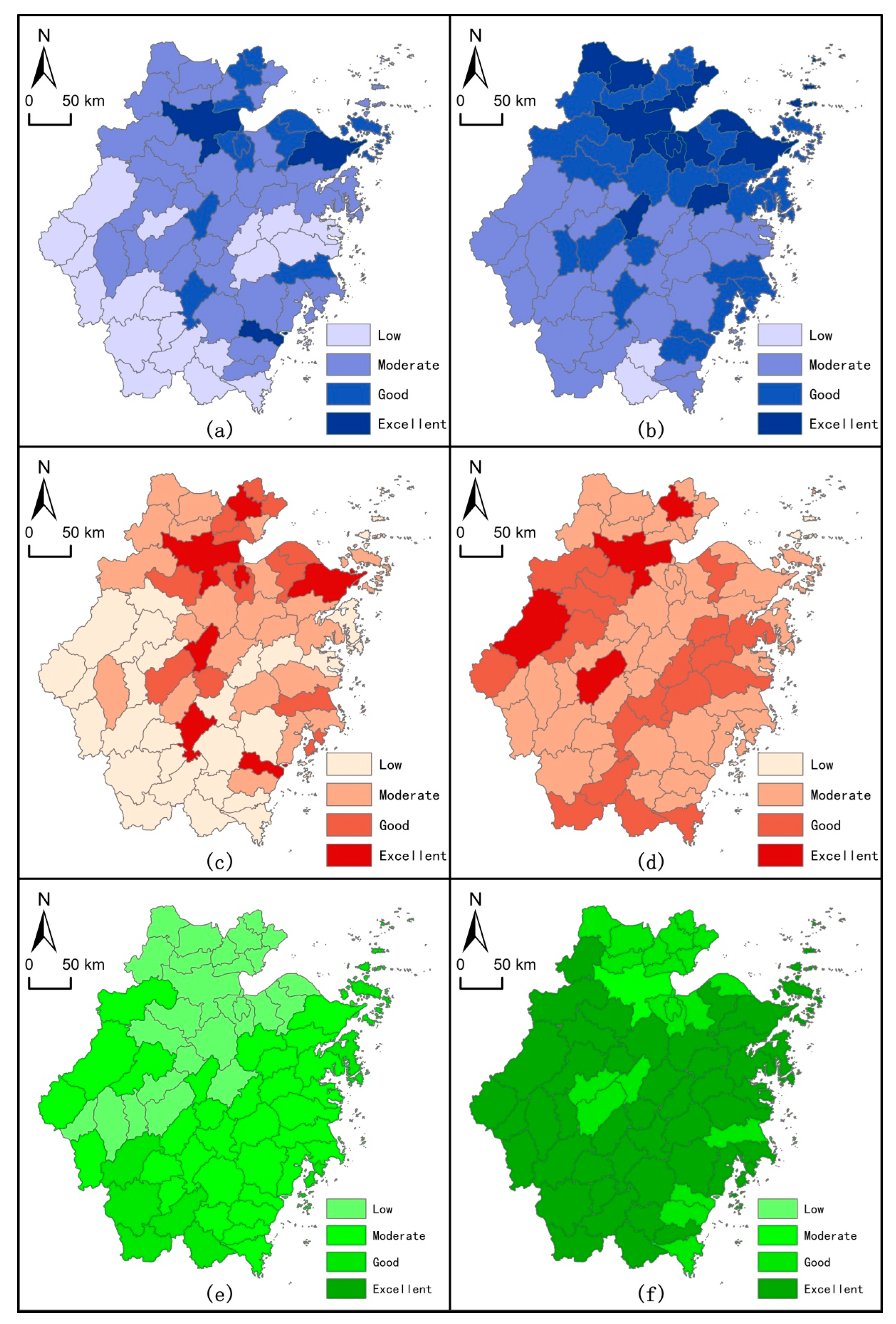
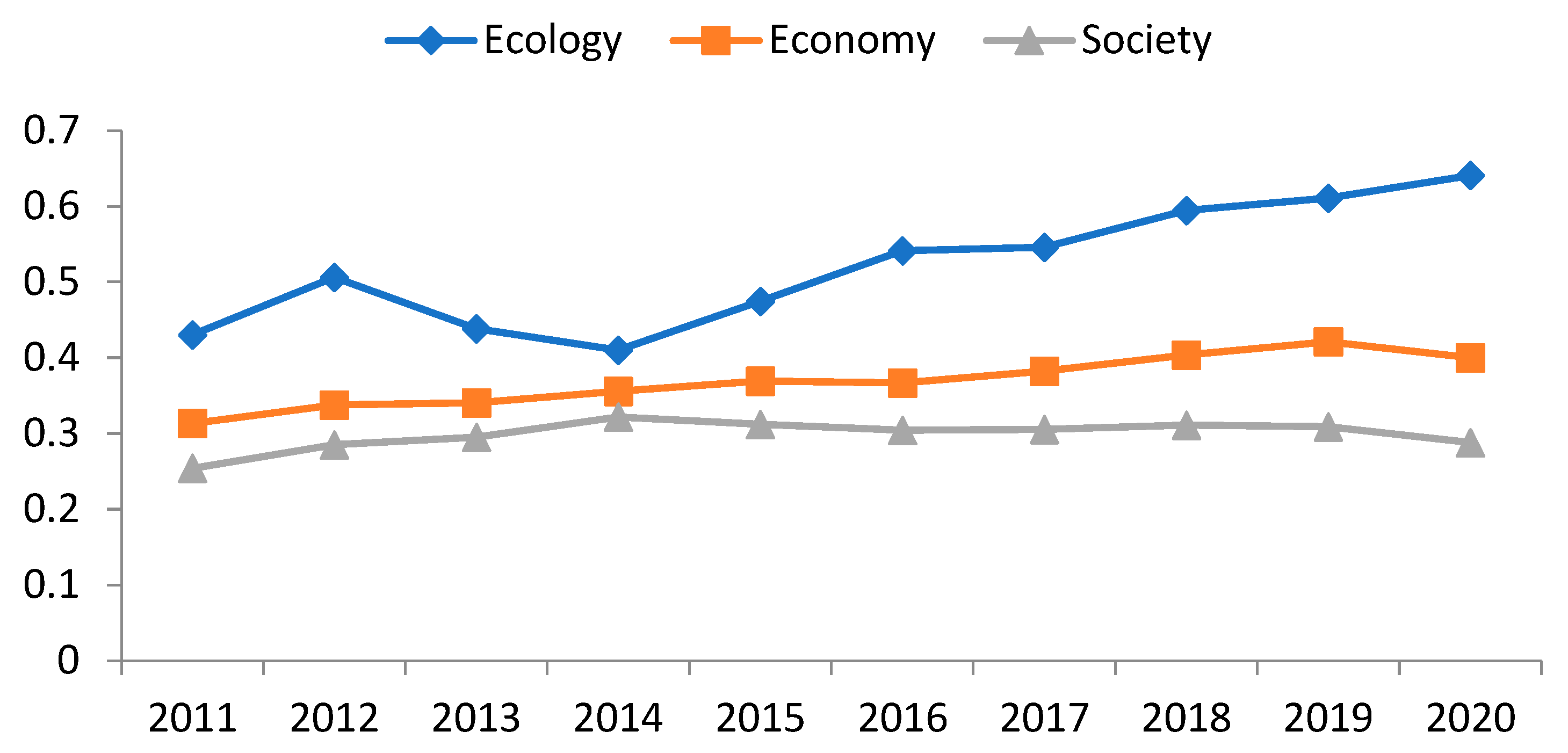
4.1. Regional Development Level Analysis

Figure 2 shows the closeness of the economic, social, and ecological systems for different cities and counties in the first year of the study period, 2011, and in the last year, 2020. As the use of the existing performance level grading method would reduce spatial differentiation, the data from each system were divided into four categories utilizing the natural interval method.

In the economic system, the high level of economic development in 2011 is mainly distributed in the northeast and southeast regions where most of the Lishui and Quzhou regions are in the low level of development, and some Ningbo and Taizhou regions are also in the low level of development; Jinhua, Wenzhou and most of the northern regions of Zhejiang Province are in the moderate level of development; and overall, only some regions of Hangzhou, Ningbo, and Wenzhou in the province are in the excellent level of development. In the economic system in 2020, all cities and counties in the province, except Wencheng and Taishun, have entered the moderate and above level in the study unit, while the excellent and good levels are mainly distributed in the northern regions, with scattered distribution in other regions, indicating a more balanced and high level of economic development compared to a decade ago, basically achieving a province-wide development of Zhejiang Province that has developed well.

In the social system, the excellent social development levels in 2011 are mainly distributed among the municipal districts of Hangzhou, Ningbo, Jiaxing, Lishui, and Wenzhou, with more than half of the districts showing low development levels, indicating a low level of social system development and a very uneven spatial distribution. In the 2020 social system, all cities and counties in the province are at the moderate and above development level, with good and excellent development levels mainly distributed in Hangzhou and Taizhou and their surrounding areas, a more balanced spatial distribution than in 2012, indicating that Zhejiang Province, in the process of economic construction, has at the same time guaranteed investment in infrastructure, social security, science, education, culture, and health, ensuring that residents can jointly enjoy the results of development.

In the ecological system, the year 2011 shows low development levels in the northern part of Zhejiang Province, indicating that in the early stages of economic and social development in Zhejiang Province, development was achieved at the expense of the ecological environment. The southwestern part of Zhejiang Province shows good and excellent development levels, showing the exact opposite spatial pattern of development performance levels compared to the economic system in 2011. In the 2020 ecological subsystem, all areas of the province except for the municipal district of Hangzhou show good and excellent development levels, with no low development levels in the province, indicating that Zhejiang Province can already transform ecology into the economy and achieve the ambitious goal of green development.

Figure 3 shows the average of the province’s closeness for the economic, social, and ecological subsystems from 2011 to 2020. In general, it shows a pattern of ecology > economy > society. Before 2014, the economic and social systems developed steadily, while the ecological subsystem showed an increase and then a decrease, indicating that the economic and social development of Zhejiang Province before that time was at the expense of the ecological environment. After 2014, the performance of the ecological subsystem and the economic system continued to improve, while the social system developed more slowly, indicating that Zhejiang Province has achieved the development model of transforming “green mountains” into “gold mountains”. The performance of the economic and social system decreases in 2020 due to a major public health event, COVID-19, which increases the burden on healthcare system and requires more financial expenditures and resources.

4.2. Regional Coordinated Development Level Analysis

4.2.1. Degree of Regional Coordinated Development

According to Figure 4, it is obvious that the coordinated development degrees of all cities and counties in Figure 4a–c have increased period by period, while Figure 4d has decreased. A large number of counties in Quzhou and Lishui in southwest Zhejiang Province have uncoordinated, barely coordinated, or primary coordination levels in 2011, while Jinhua, Shaoxing, Ningbo, Hangzhou, Huzhou, and Jiaxing in the north-central region have reached good coordination or high-quality. In 2014, only four counties in the province, namely Taishun, Wencheng, Qingyuan, and Jingning, were at the primary level of coordination, while all other areas reached the intermediate level of coordination or above, indicating that every city and county in the province was at the primary level of coordination and above at this time. In 2017, compared to 2014, there was further development, with all cities and counties in the province reaching a moderate level of coordination and above, at which point a pattern of development with a high level of coordination in each region was formed. It is of concern that in 2020, the level of economic and social development declined due to major public health events and, therefore, some regions experienced a decline in coordination.

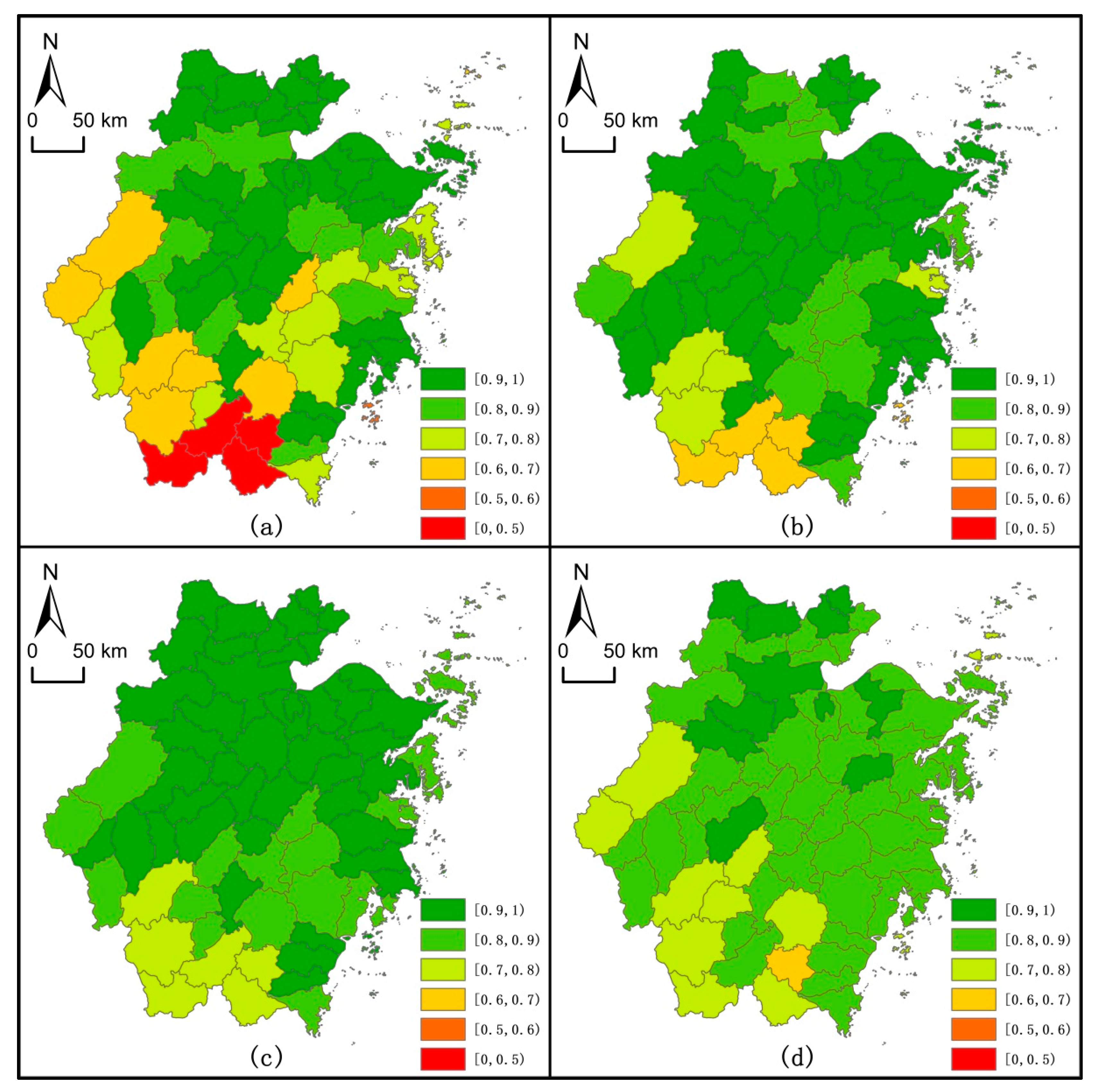
4.2.2. Regional Coordinated Development Level

Figure 5 shows the spatial pattern in the level of RCD in Zhejiang Province in 2011, 2014, 2017, and 2020. In 2011, most of the province’s RCD was less than 0.5, in the slight or moderate dysfunctional recession category in the RCD ranking, but no county or city in the province was in the severe dysfunctional recession category. The province’s RCD in 2014 showed a very significant improvement compared to 2011, but there were still more areas in the dysfunctional decline category. In 2017, only two counties in the province were in the dysfunctional decline category, showing a predominantly well-coordinated pattern of spatial development, indicating that the province’s RCD had improved to a greater extent by this time, but the region was still in a process of dysfunctional decline. In 2020, only one county in the province was in the slightly dysfunctional decline category and two counties were in the intermediate coordinated development category, while the rest of the areas were in the good and above coordinated development category, indicating that the development results had been further consolidated, the RCDs of cities and counties in the province had tended to equalize, and all areas were enjoying the fruits of the coordinated development of the economic–social–ecological system.

4.3. Regional Differences Analysis

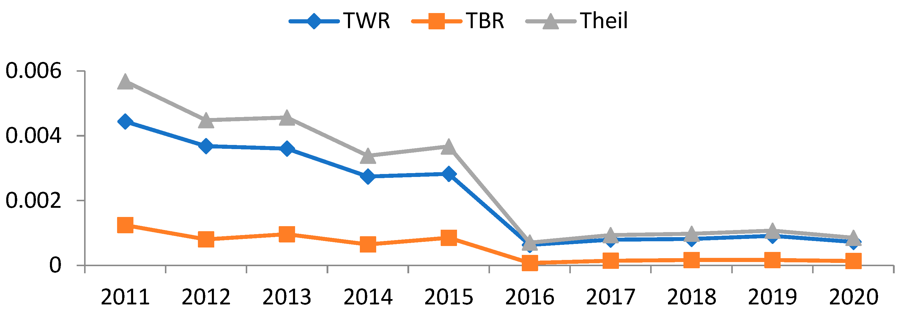
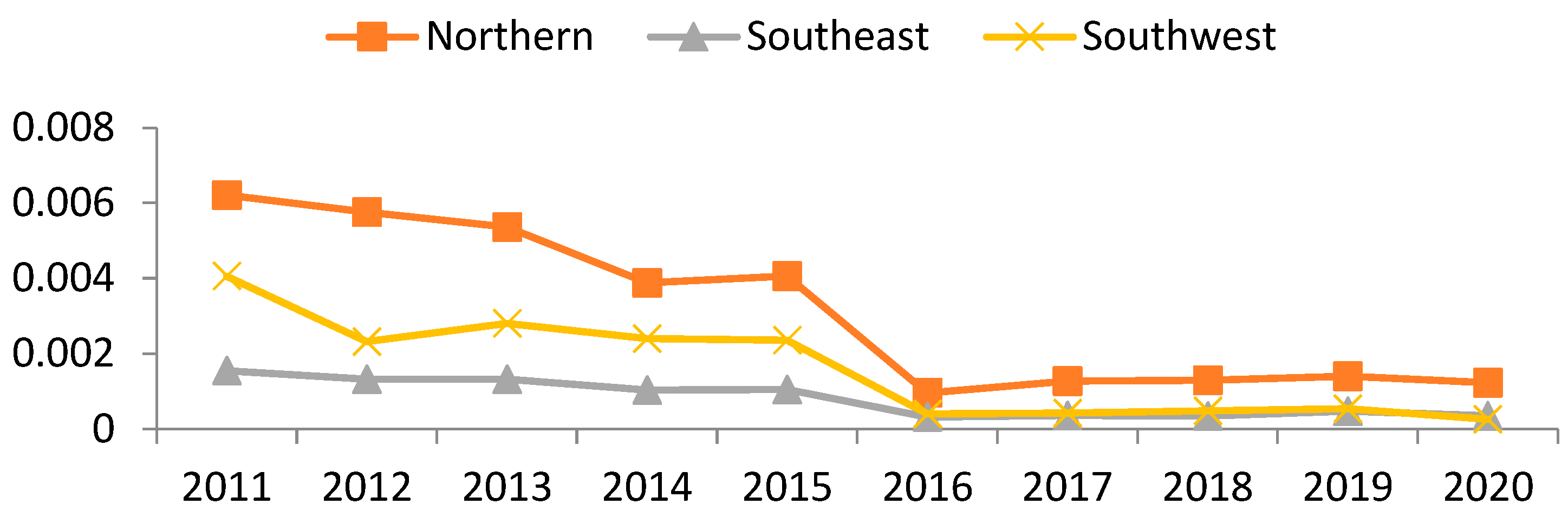
4.3.1. Intra- and Inter-Regional RCD Differences Analysis

The results from the measurement of the Theil index of the RCD in this study are shown in

Table 6. Overall RCD difference and its decomposition in Zhejiang Province from 2011 to 2020.

Year	TWR	TBR	Theil	WW	Wb
2011	0.00444	0.00124	0.00568	0.78185	0.21815
2012	0.00368	0.00080	0.00448	0.82046	0.17954
2013	0.00360	0.00096	0.00456	0.79015	0.20985
2014	0.00274	0.00064	0.00338	0.81014	0.18986
2015	0.00282	0.00085	0.00367	0.76846	0.23154
2016	0.00063	0.00007	0.00070	0.89657	0.10343
2017	0.00079	0.00014	0.00093	0.84619	0.15381
2018	0.00081	0.00016	0.00097	0.83804	0.16196
2019	0.00091	0.00016	0.00107	0.84848	0.15152
2020	0.00072	0.00013	0.00085	0.85088	0.14912

. Meanwhile, the trend of the overall, inter-, and intra-Theil index in Zhejiang Province from 2011 to 2020 as Figure 6, which portrays the RCD differences of each region.

Figure 6 shows the intra-regional Theil index curve is the same as the overall Theil index curve, with the overall trend showing fluctuations and decreases, with a declining phase until 2015, with the largest decrease in 2015, after which it tends to stabilize, indicating that the differences in RCD between different cities and counties within the three regions of Zhejiang Province first gradually decrease and then stabilize. The trend of the inter-regional Theil index curve is similar to the overall Theil index curve, but the change is smaller and always significantly lower than the intra-regional Theil index compared to the intra-regional differences.

In terms of contribution to the overall difference (Table 6), the intra-regional contribution (around 80%) is always much larger than the inter-regional contribution, which means that the main cause of the regional difference is still the RCD difference within the three regions.

4.3.2. Spatial Differentiation Characteristics

The Theil index and its contribution to the overall Theil index within each of the three regions (the north, southwest, and southeast) are calculated using the formula as shown in Figure 7 and

Table 7. Differences and contribution rates within each of the three regions from 2011 to 2020.

Year	Northern	Southeast	Southwest	Wnorthern	Wsoutheast	Wsouthwest
2011	0.00621	0.00155	0.00406	0.36127	0.18919	0.23138
2012	0.00576	0.00132	0.00232	0.37964	0.19444	0.24638
2013	0.00536	0.00132	0.00280	0.35930	0.19364	0.23720
2014	0.00388	0.00103	0.00240	0.36822	0.19622	0.24570
2015	0.00406	0.00105	0.00236	0.35269	0.18523	0.23053
2016	0.00096	0.00032	0.00040	0.40442	0.21100	0.28115
2017	0.00127	0.00036	0.00042	0.38306	0.19979	0.26334
2018	0.00129	0.00034	0.00048	0.37901	0.19840	0.26064
2019	0.00140	0.00047	0.00054	0.38311	0.20137	0.26400
2020	0.00123	0.00035	0.00026	0.38778	0.19783	0.26527

.

The results show that the magnitude of the Theil index within each region is largely different, while the trend in the change is largely the same, with all decreasing more sharply in 2016 and then remaining stable. However, the Theil index in the north is consistently greater than that in the southeast and southwest, indicating that the differences in coordinated development between the regions were narrowing after all the policies were implemented in 2016. In the north, the Theil index had its first significant drop in 2014. In the southwest region, the Theil index had its first significant decrease in 2012, indicating that regional differences were narrowing earlier than in the north region. In the southeast, the overall decline in the Theil index was more gradual than in the north and southwest regions. In terms of contribution to the overall Theil index, the north is consistently larger than the southwest and southeast regions, while both southern regions are closer in contribution (nearly 20%).

4.4. Spatial Pattern Analysis

4.4.1. Global Spatial Autocorrelation Analysis

According to the geographical spatial relationship of the 58 counties and 11 cities, using Geoda software with spatial weights based on queen contiguity, the global Moran’s I for RCD was calculated from 2011 to 2020 [39]. The results are shown in

Table 8. Global Moran’s index statistics of RCD from 2011 to 2020.

Year	Moran’s I	E(I)	Z Score	p Value
2011	0.425	−0.0193	5.5167	0.001
2012	0.451	−0.0156	5.8532	0.001
2013	0.406	−0.0156	5.3123	0.001
2014	0.364	−0.0156	4.8046	0.001
2015	0.422	−0.0156	5.5257	0.001
2016	0.314	−0.0156	4.1347	0.001
2017	0.358	−0.0156	4.6830	0.001
2018	0.361	−0.0156	4.7271	0.001
2019	0.321	−0.0156	4.1867	0.001
2020	0.356	−0.0156	4.7383	0.001

. The global Moran’s I values are all positive numbers larger than 0.3, and all results were positive at the 1% significance level for every year, which demonstrates spatial cluster patterns that indicate most counties and cities experienced a significant spatial correlation for RCD. In other words, RCD is prominently correlated to the values of its neighboring counties and cities.

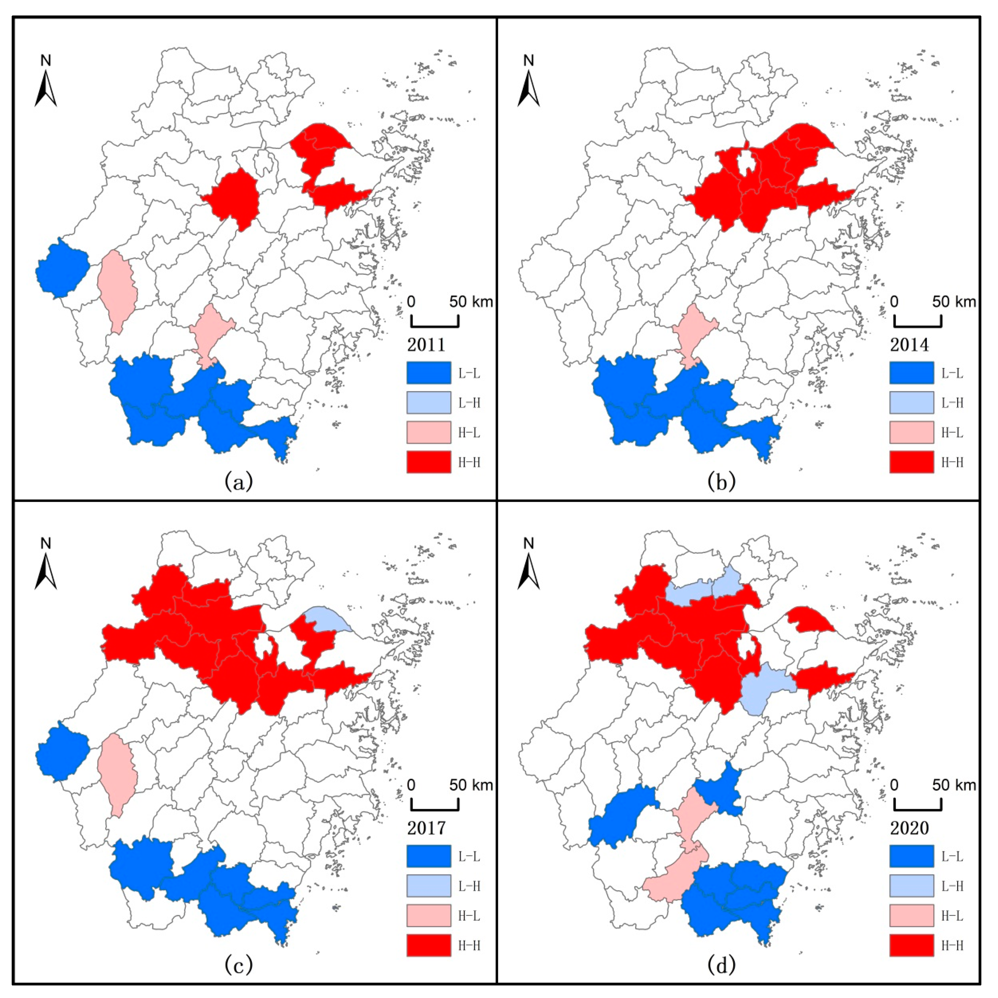
4.4.2. Local Spatial Autocorrelation Analysis

This analysis uses Equation (26) to measure the local Moran’s I for RCD for the years 2011, 2014, 2017, and 2020. As is shown in Figure 8, it can be divided into the following four types.

(1) High–High agglomeration area (H-H correlation). It is mainly located in northern Zhejiang, with a high distribution in prefecture-level cities such as Hangzhou, Shaoxing, Ningbo, Jiaxing, and Huzhou, and a high RCD in both this category and its surrounding areas. The RCD of cities and counties in the region is at a high level due to a combination of factors such as a high level of economic development, strong comprehensive social development capacity, and the environmental management system, and has a strong positive driving effect on the surrounding cities, with significant spatial spillover effects.

(2) High-value heterogeneity area (H-L correlation). It is mainly concentrated in Lishui and Quzhou, both of which have a much higher RCD than the surrounding regions. These regions are dominated by counties in southwest Zhejiang, which have more obvious advantages in terms of resource endowment, promoting green economic development and social development, resulting in a high level of coordinated development of the economy, society, and ecology in the region, but the scale of the counties is small, and the driving and radiating effect on the surrounding areas is not strong.

(3) Low-value heterogeneity area (L-H correlation). The only areas in this category exist in 2017 and 2020 and are mainly spatially scattered in northern Zhejiang. The RCD for this type of area is much lower than the RCD of its surrounding cities or counties. The RCD of this category is much lower than the RCD of its surrounding cities or counties, which are located around diffuse effect areas with high RCD but have limited ability to breed receptive diffuse effect areas, resulting in a low RCD, so there is more room for improvement in this category.

(4) Low–Low agglomeration area (L-L correlation). It is mainly concentrated in the southern part of Zhejiang, namely in the counties of Wenzhou and southern Lishui. The RCD is low in both this category and its surrounding areas. Although the Lishui region has a high level of ecological environment, it cannot adequately transform ecological resources into a driving force for economic and social development. Although the Wenzhou area has been able to improve its level of economic development and social development capacity through some heavy chemical industries and highly polluting and energy-consuming manufacturing industries, the problems of environmental pollution and ecological damage are more obvious.

5. Conclusions and Policy Recommendations

5.1. Conclusions

To sum up, the development of Zhejiang Province in the last decade provides evidence of its role as a demonstration zone for common prosperity. Based on the spatial panel data from 11 cities and 58 counties in Zhejiang Province from 2011 to 2020, the PCA-TOPSIS model is constructed to measure the development levels of their economic, social, and ecological subsystems, and the coordinated development model is applied to measure the degree of regional coordinated development in each study unit to explore the spatial and temporal evolution patterns of Zhejiang Province as a demonstration zone of common prosperity in terms of regional coordinated development.

The regional differences and spatial agglomeration pattern of coordinated regional development are portrayed through the Theil index and exploratory spatial data analysis methods. The main results of this study include: (1) In terms of temporal development, all cities or counties show a continuous or fluctuating increase in the three subsystems of economy, society, and ecology, and the level of coordinated regional development in each study unit also shows an upward trend. It shows that steady regional development is the fundamental material basis for common prosperity. (2) In terms of spatial evolution, the level of economic and social development is high in the north and low in the south, and the level of ecological development is high in the south and low in the north, and the level of coordinated regional development evolves from a very uneven spatial distribution to a level of good in the majority of cities. It shows that the equalization of development among regions is a realistic manifestation of common prosperity. (3) In terms of regional differences, the differences in the level of coordinated regional development are greater than those between regions, with the differences in the north being greater than those in the south, and, in general, the differences between regions are narrowing. (4) In terms of spatial correlation, the level of coordinated regional development shows a significant positive correlation, with high-value areas tending to be adjacent to high-value areas and low-value areas tending to be adjacent to low-value areas. In sum, the development of Zhejiang Province in the last decade provides evidence of its role as a demonstration zone for common prosperity. It confirms that coordinated regional development is the fundamental way to achieve common prosperity. (5) Based on the weights of the indicators in the evaluation index system, it is found that economic strength is particularly important in the economic subsystem. The level of health care and information technology are important paths to improve infrastructure. Medical service and unemployment insurance are important components of social security. Ensuring the steady implementation of primary and secondary education is necessary to improve the performance of the social subsystem. In the ecological subsystem, environmental quality is the top priority for improving ecological performance, such as the improved air quality.

5.2. Policy Recommendations

This study deeply explores the path of coordinated regional development to achieve common prosperity by measuring and analyzing the spatial and temporal patterns of RCD levels in common prosperity demonstration areas. By combining regional policies implemented in economic, social, and ecological subsystems, Zhejiang Province provides empirical references and policy improvement suggestions for other regions in China.

5.2.1. Economic Perspective

The government can consolidate the economic foundation, improve the economic structure, and promote economic efficiency. Economic development is the fundamental material basis for common prosperity. The government can stabilize the economic growth rate, realize digitalization, automation, and intelligence in the manufacturing industry, promote county manufacturing cooperation, safeguard local advantages, and cultivate specialized manufacturing industry clusters. The government can promote the transformation of scientific and technological achievements into industries, realize agricultural intensification, mechanization, and refinement, build agricultural parks with industry-village interaction and ecological recycling, and promote the integration of agriculture with manufacturing and service industries. The government can build production factors and information exchange networks inside and outside the sea, land, and air to solve the problem of difficult movement of population, capital, and technology to the grassroots and improve the efficiency of economic circulation. The government can take advantage of regional advantages, strengthen the division of labor and cooperation, and actively integrate with the integration and development of central cities. The government can stimulate market vitality, implement market-oriented reforms for state-owned enterprises, simplify and decentralize the government for private enterprises, and implement anti-monopoly regulation for the platform economy.

5.2.2. Social Perspective

The government can strengthen public services, improve the social security system, and focus on social equity. To narrow the regional development gap between urban and rural areas and counties, the primary task is to equalize and integrate basic public services, improve the quality of public services, continuously improve the conditions of transportation, education, medical care, and housing in relatively less developed areas, and achieve equality in education in different regions. The government can improve the social security system, compel enterprises to establish five insurance and one fund, popularize urban and rural health insurance, and establish employment assistance and unemployment subsidies using transfer payments and other means. The government can emphasize the development of science and technology, improve the level of knowledge, promote the transformation of scientific and technological achievements and technology transactions, and focus on fostering industries such as new materials, new energy, information technology, and biotechnology.

5.2.3. Ecological Perspective

The government can adhere to green development, conserve and intensify land use, and protect green water and green mountains. It can strictly implement ecological environmental protection policies and explore the green development path of transforming “green water and green hills” into “golden mountains” according to local conditions. The government can promote the green transformation of production and lifestyle, actively develop carbon trading, green finance, and other green industries, promote the development of the green economy, and realize energy saving and emission reduction. The government can deepen the implementation of arable land protection and land conservation systems, improve the quality and quantity of arable land, improve the stock of construction land, curb urban disorderly expansion, and promote the optimal accumulation of urban-scale construction. The government can promote the formation of an eco-economy-oriented governance system for common prosperity with a focus on coordinated economic-social-ecological development.

5.3. Limitations and Future Research

It is worth pointing out that this paper only corroborates the empirical evidence of Zhejiang Province as a model area of common prosperity through coordinated regional development, and the common prosperity can be evaluated in future studies from the perspectives of urban–rural development differences and high-quality development. Meanwhile, the drivers of common prosperity can be explored, such as economic growth, distribution system, science and technology innovation, etc.

References

1. Liu, L. The Construction of China’s Social Governance Community and Solid Promotion of Common Prosperity. Reform 2022, 8, 87–97. (In Chinese) [Google Scholar]
2. Ma, H. “Common Prosperity” in the Historical Logic of Marxism. Philos. Anal. 2022, 13, 98–110+198. (In Chinese) [Google Scholar]
3. Dong, X.; Li, J.; Chi, R. A Study on Xi Jingpin’s Important Expositions on Coordinated Regional Development. J. Zhejiang Univ. (Humanit. Soc. Sci.) 2019, 49, 16–28. (In Chinese) [Google Scholar]
4. Zhu, X.-G.; Li, T.; Feng, T.-T. On the Synergy in the Sustainable Development of Cultural Landscape in Traditional Villages under the Measure of Balanced Development Index: Case Study of the Zhejiang Province. Sustainability 2022, 14, 11367. [Google Scholar] [CrossRef]
5. Qin, C.; Zheng, Y.; Zhang, H. A Study on the Tendencies and Features of the Coordinated Development of Regional Economy in China. Econ. Geogr. 2013, 33, 9–14. [Google Scholar] [CrossRef]
6. Yang, Q. Measurement of China’s “Five Transformations” and its Spatial Pattern of Coordinated Development. China Agric. 2017, 10, 203–209. [Google Scholar] [CrossRef]
7. Ruan, Y.; Xu, B. Measurement and evaluation of the degree of coordinated development of urban and rural areas. Stat. Decis. Mak. 2017, 19, 136–138. [Google Scholar] [CrossRef]
8. Deng, H.; Cao, Y. Coordinated Development Performance in China. Reg. Econ. Rev. 2019, 1, 25–32. [Google Scholar] [CrossRef]
9. Chen, L.; Yu, J.; Xu, Y. Construction of the Common Prosperity Index Model. Gov. Stud. 2021, 37, 5–16+2. [Google Scholar] [CrossRef]
10. Ren, Z.L. Evaluation Method of Port Enterprise Product Quality Based on Entropy Weight TOPSIS. J. Coast. Res. 2020, 103, 766–769. [Google Scholar] [CrossRef]
11. de Cheveigne, A. Quadratic component analysis. Neuroimage 2012, 59, 3838–3844. [Google Scholar] [CrossRef] [PubMed]
12. Alaoui, Y.L.; Tkiouat, M. Assessing the performance of microfinance lending process using AHP-fuzzy comprehensive evaluation method: Moroccan case study. Int. J. Eng. Bus. Manag. 2017, 9. [Google Scholar] [CrossRef]
13. Cao, W.; Zhang, X.; Pan, Y.; Zhang, C. Coordinate Development among Population, Land and Economy Urbanization in Developed Area: The Case of Jiangsu Province. China Popul. Resour. Environ. 2012, 22, 141–146. (In Chinese) [Google Scholar]
14. Malakar, K.; Mishra, T. Application of Gini, Theil and concentration indices for assessing water use inequality. Int. J. Soc. Econ. 2017, 44, 1335–1347. [Google Scholar] [CrossRef]
15. Chakravarty, S.R.; Silber, J. A generalized index of employment segregation. Math. Soc. Sci. 2007, 53, 185–195. [Google Scholar] [CrossRef]
16. Barvels, E.; Fensholt, R. Earth Observation-Based Detectability of the Effects of Land Management Programmes to Counter Land Degradation: A Case Study from the Highlands of the Ethiopian Plateau. Remote Sens. 2021, 13, 1297. [Google Scholar] [CrossRef]
17. Sun, Y.; Shen, S. The spatio-temporal evolutionary pattern and driving forces mechanism of green technology innovation efficiency in the Yangtze River Delta region. Geogr. Res. 2021, 40, 2743–2759. (In Chinese) [Google Scholar]
18. Munibah, K.; Widiatmaka, W.; Widjaja, H. Spatial Autocorrelation on Public Facility Availability Index with Neighborhoods Weight Difference. J. Reg. City Plan. 2018, 29, 18–31. [Google Scholar] [CrossRef]
19. Lu, Q.; Yang, Y.; Li, B.; Li, Y.; Wang, D. Coupling Relationship and Influencing Factors of the Water-Energy-Cotton System in Tarim River Basin. Agronomy 2022, 12, 2333. [Google Scholar] [CrossRef]
20. Huang, H.; Zou, C.; Cao, J.; Tsang, P.; Zhu, F.; Yu, C.; Xue, S. Water-soluble Ions in PM2.5 on the Qianhu Campus of Nanchang University, Nanchang City: Indoor-Outdoor Distribution and Source Implications. Aerosol Air Qual. Res. 2012, 12, 435–443. [Google Scholar] [CrossRef]
21. Zheng, Y.; Xuehua, Z. Principal component method in analysis of water resources sustainability influence factors. In Proceedings of the 2009 International Conference on Management and Service Science, Beijing, China, 20–22 September 2009; p. 4. [Google Scholar]
22. An, H.; Xu, J.; Ma, X. Does technological progress and industrial structure reduce electricity consumption? Evidence from spatial and heterogeneity analysis. Struct. Change Econ. Dyn. 2020, 52, 206–220. [Google Scholar] [CrossRef]
23. Jiaxing, Z.; Lin, L.; Hang, L.; Dongmei, P. Evaluation and analysis on suitability of human settlement environment in Qingdao. PLoS ONE 2021, 16, e0256502. [Google Scholar] [CrossRef] [PubMed]
24. Zavadskas, E.K.; Mardani, A.; Turskis, Z.; Jusoh, A.; Nor, K.M.D. Development of TOPSIS Method to Solve Complicated Decision-Making Problems: An Overview on Developments from 2000 to 2015. Int. J. Inf. Technol. Decis. Mak. 2016, 15, 645–682. [Google Scholar] [CrossRef]
25. Ishizaka, A.; Balkenborg, D.; Kaplan, T. Does AHP help us make a choice? An experimental evaluation. J. Oper. Res. Soc. 2011, 62, 1801–1812. [Google Scholar] [CrossRef]
26. Chen, C.; Zhang, Y.; An, J.G.; He, Y.; Gong, X. Comparative Study of Four Maxillofacial Trauma Scoring Systems and Expert Score. J. Oral Maxillofac. Surg. 2014, 72, 2212–2220. [Google Scholar] [CrossRef]
27. Liwicki, S.; Tzimiropoulos, G.; Zafeiriou, S.; Pantic, M. Euler Principal Component Analysis. Int. J. Comput. Vis. 2013, 101, 498–518. [Google Scholar] [CrossRef]
28. Choulakian, V. Robust Q-mode principal component analysis in L-1. Comput. Stat. Data Anal. 2001, 37, 135–150. [Google Scholar] [CrossRef]
29. Jiang, B. Head/Tail Breaks: A New Classification Scheme for Data with a Heavy-Tailed Distribution. Prof. Geogr. 2013, 65, 482–494. [Google Scholar] [CrossRef]
30. Zhu, S.; Xu, B.; Mao, J. The evaluation on urban ecosystem health and its obstacle degree: A case study on Nanning City. J. Anhui Univeisity (Nat. Sci. Ed.) 2015, 39, 96–102. (In Chinese) [Google Scholar]
31. Jiang, X.; Wu, X. Quantitative investigation of the coordinated development of ecology-economysociety in forest resource-based city: A case study of Yichun, Heilongjiang Province. Acta Ecol. Sin. 2021, 41, 8396–8407. (In Chinese) [Google Scholar]
32. Liao, C. Quantitaitve Judgement and Classification System for Coordinated Development of Environment Amd Economy—A Case Study of the City Group in the Pearl River Delta. Trop. Geography. 1999, 19, 76–82. (In Chinese) [Google Scholar]
33. Cheng, C.; Liu, Y.L.; Liu, Y.F.; Yang, R.F.; Hong, Y.S.; Lu, Y.C.; Pan, J.W.; Chen, Y.Y. Cropland use sustainability in Cheng-Yu Urban Agglomeration, China: Evaluation framework, driving factors and development paths. J. Clean. Prod. 2020, 256, 120692. [Google Scholar] [CrossRef]
34. Sun, F.; Ye, C. Modelling of the environmental sustainability assessment index for inhabited islands. Earth Sci. Inform. 2022, 15, 1385–1394. [Google Scholar] [CrossRef]
35. Cui, Y.; Khan, S.U.; Sauer, J.; Zhao, M. Exploring the spatiotemporal heterogeneity and influencing factors of agricultural carbon footprint and carbon footprint intensity: Embodying carbon sink effect. Sci. Total Environ. 2022, 846, 157507. [Google Scholar] [CrossRef] [PubMed]
36. Li, R.; Sun, T. Research on Measurement of Regional Differences and Decomposition of Influencing Factors of Carbon Emissions of China’s Logistics Industry. Pol. J. Environ. Stud. 2021, 30, 3137–3150. [Google Scholar] [CrossRef]
37. Yu, X.; Gong, S.; Wu, Y. Spatial Statistical Analysis on the Variability of County Economies in Zhejiang Province. Areal Res. Dev. 2012, 31, 27–32. (In Chinese) [Google Scholar]
38. Zhang, W.; Wang, B.; Wang, J.; Wu, Q.; Wei, Y.D. How does industrial agglomeration affect urban land use efficiency? A spatial analysis of Chinese cities. Land Use Policy 2022, 119, 106178. [Google Scholar] [CrossRef]
39. Kumari, M.; Sarma, K.; Sharma, R. Using Moran’s I and GIS to study the spatial pattern of land surface temperature in relation to land use/cover around a thermal power plant in Singrauli district, Madhya Pradesh, India. Remote Sens. Appl. Soc. Environ. 2019, 15, 100239. [Google Scholar] [CrossRef]
Figure 1. Geographical location of the study area.
Sustainability 15 02939 g001
Figure 2. Results for the closeness of the economic, social, and ecological systems in 11 cities and 58 counties in the Zhejiang Province in 2011 and 2020. (a) Results for the closeness of the economic system in 2011. (b) Results for the closeness of the economic system in 2020. (c) Results for the closeness of the social system in 2011. (d) Results for the closeness of the social system in 2020. (e) Results for the closeness of the ecological system in 2011. (f) Results for the closeness of the ecological system in 2020.
Sustainability 15 02939 g002
Figure 3. The average of the province’s closeness for the subsystems from 2011 to 2020.
Sustainability 15 02939 g003
Figure 4. The degree of Regional Coordinated Development of Zhejiang Province in 2011, 2014, 2017, and 2020. (a) Results for the degree of RCD in 2011. (b) Results for the degree of RCD in 2014. (c) Results for the degree of RCD in 2017. (d) Results for the degree of RCD in 2020.
Sustainability 15 02939 g004
Figure 5. The Regional Coordinated Development of Zhejiang Province in 2011, 2014, 2017, and 2020. (a) Results for the RCD in 2011. (b) Results for the RCD in 2014. (c) Results for the RCD in 2017. (d) Results for the RCD in 2020.
Sustainability 15 02939 g005
Figure 6. Overall Theil index and its decomposition in Zhejiang Province from 2011 to 2020.
Sustainability 15 02939 g006
Figure 7. Differences within each of the three regions from 2011 to 2020.
Sustainability 15 02939 g007
Figure 8. LISA concentration diagram of RCD in the main years. (a) LISA concentration diagram of RCD in 2011. (b) LISA concentration diagram of RCD in 2014. (c) LISA concentration diagram of RCD in 2017. (d) LISA concentration diagram of RCD in 2020.
Sustainability 15 02939 g008