Solar Self-Sufficient Households as a Driving Factor for Sustainability Transformation

Abstract

We present a model to estimate the technical requirements, including the photovoltaic area and battery capacity, along with the costs, for a four-person household to be 100% electrically self-sufficient in Germany. We model the hourly electricity consumption of private households with quasi-Fourier series and an autoregressive statistical model based on data from Berlin in 2010. Combining the consumption model and remote-sensed hourly solar irradiance data from the ERA5 data set, we find the optimal photovoltaic area and battery capacity that would have been necessary to be self-sufficient in electricity from July 2002 to June 2022. We show that it is possible to build a self-sufficient household with today’s storage technology for private households and estimate the costs expected to do so.

1. Introduction

Two of the Sustainable Development Goals (SDGs) declared by the UN are to “take urgent action to combat climate change and its impacts” [1] and to “ensure access to affordable, reliable, sustainable, and modern energy for all” [2]. These goals are expected to be fulfilled by 2030. Strategies to fulfill these goals can be categorized into top–down and bottom–up approaches [3]. An example of a top–down approach would be the decision of governments to ban CFCs [4]. An example of a bottom–up process is the population-driven evolution of individual commitments to a more sustainable vegan diet [5,6,7]. Top–down and bottom–up approaches are not mutually exclusive and can even complement each other. Thus, the efforts of governments to transform entire countries and economies toward sustainability can and should be supported by individuals within the population.

For the transformation toward sustainability, solar self-sufficiency is of special interest for a number of reasons. First, in Germany, 89% of suitable roof areas are still unused [8]. Second, prices for solar power systems and battery storage continue to drop [9], and the materials are becoming more sustainable due to the increased use of natural materials [10]. For this paper, 31 interviews were carried out with solar and battery installers to understand the customer requests and needs and the market products. These interviews revealed that the number of requests for information about self-sufficiency in particular was unusually high this year. Moreover, we found that installers did not have a neutral source of information about the actual requirements for sizing photovoltaic systems and batteries to be self-sufficient. This unusual level of interest could be due to the current media-promoted energy uncertainty [11] and the sharp increase in electricity costs in Germany in 2022 (the wholesale electricity price rose from 128 EUR/MWh in February 2022 to 469 EUR/MWh in August 2022 [12]).

Research on self-sufficiency and 100% renewable energy has a long history (e.g., [13,14,15,16,17,18,19]). One major branch of the literature focuses on how communities, cities, or countries can become energy self-sufficient. For example, the economic, ecological, social, and energy system factors driving municipal governments to seek energy self-sufficiency were analyzed [20]. Ram et al. [21] proposed a pathway for a policy-driven transition to self-sufficiency for the city of Delhi. Moreover, Oyewo et al. [22] showed how South Africa can make the transition to 100% renewable energy by 2050.

Another branch of the research focuses on cost-optimization modeling for private households. The economically optimal photovoltaic (PV) modules for private households in South Korea have a power output of about $1.2$ kW [23] (kW kilowatt). In Spain and France, under the assumption that the electricity is only self-consumed, so neither stored nor fed into the grid, the economically optimal PV modules have a power of about $1.5$ kWp [24] (kWp kilowatt peak, indicates the power of the modules under standard conditions, 25 °C module temperature, 1000 W/m${}^2$ solar irradiance). A map with the estimated economically optimal PV areas and costs for 145 countries can be found in [25]. Research has also been conducted into the economically optimal battery capacity, which is about 1–5 kWh for private households in Spain (kWh kilowatt hour) [26].

A third branch of the self-sufficiency literature is the estimation of the degree of self-sufficiency. A degree of self-sufficiency of about 30% was reached in a model of a Polish city, in which all rooftops were assumed to be covered with PV modules [27]. Furthermore, Mutani and Todeschi [28] showed a degree of self-sufficiency of about $40\%$ under optimal orientation of the PV modules for private households in Spain. A degree of $68\%$ was achieved in a household in Slovenia which was powered by PV modules in combination with a hydrogen battery [29]. The consumption and production was measured in 15-min intervals for one year. Recently, a research study on households in Iraq showed that it is possible to achieve a self-sufficiency degree of about $83\%$ using PV modules in combination with batteries [30].

Regarding the trade-off between the cost optimization and the degree of self-sufficiency, Colmenar-Santos et al. [31] demonstrated that 100% solar self-sufficiency is not the economic optimum. However, homeowners are often willing to pay a premium for self-sufficiency [32]. However, there is a lack of research and information on the requirements to obtain 100% solar self-sufficiency for private households and the associated costs, even though there has been research decades ago on this topic. Lund [33] showed in 1991 a standalone photovoltaic-hydrogen energy system that was able to produce constantly 1 kW output power. A 100% energy self-sufficient house was build by research teams in Freiburg, Germany in 1994 [34]. Although this represents a great success for self-sufficiency research, it must be said that the effort required to achieve this goal will not be expendable for private households.

Today, there are websites run by public providers that can be used to estimate the expected annual electricity production for certain parameters [35,36]. These tools either calculate only the electricity production without comparison to a consumption curve or are restrictive in the choice of parameters so that parameter sets for achieving 100% solar self-sufficiency are not allowed. On the whole, there is a lack of information for private households on the requirements and possible investments to achieve 100% solar self-sufficiency.

In this paper, our goal is to contribute to the energy sustainability transformation by presenting a model that can be used to estimate photovoltaic module size (PV area) and maximum battery capacity (MBC) requirements for solar self-sufficiency for private households. We derive our model by optimizing the required PV area and MBC in different regions of Germany, which receive different amounts of solar radiation. The optimization is performed under the constraint that the hourly consumption and production of electricity never empties the home battery. We then use our model with current price levels to derive the average annual cost of solar self-sufficiency. We do not attempt to predict electricity production and consumption (for studies on these, see [37,38,39]). Instead, we model hourly annual consumption using representative data from Berlin, Germany in 2010 [40]. To calculate potential electricity production, we use reanalysis data on a raster map between July 2002 and June 2022 (ERA5, [41]). Furthermore, we use these data sources to optimize for the minimal required PV area and MBC for self-sufficiency over the last 20 years in Germany.

The paper is organized as follows. First, we discuss our data sources in Section 2. Then, in Section 3, we outline the model of electricity consumption and the method of optimization to derive the PV area and MBC that would have been needed for self-sufficiency over the past 20 years. Section 4 presents the results, including a colored map of Germany indicating the best and worst regions for solar self-sufficiency, the relationship between required battery capacity and available PV area, and a model for the additional costs that are to be expected. In particular, it shows that it is possible to achieve self-sufficiency with today’s storage technology. Finally, Section 5 summarizes the results and concludes the paper with the discussion of potential further improvements of our model.

2. Production–Consumption Cycle and Data Description

In this section, we introduce the production–consumption cycle of electrical energy. Then, we use the components of the cycle to structure the description of the data.

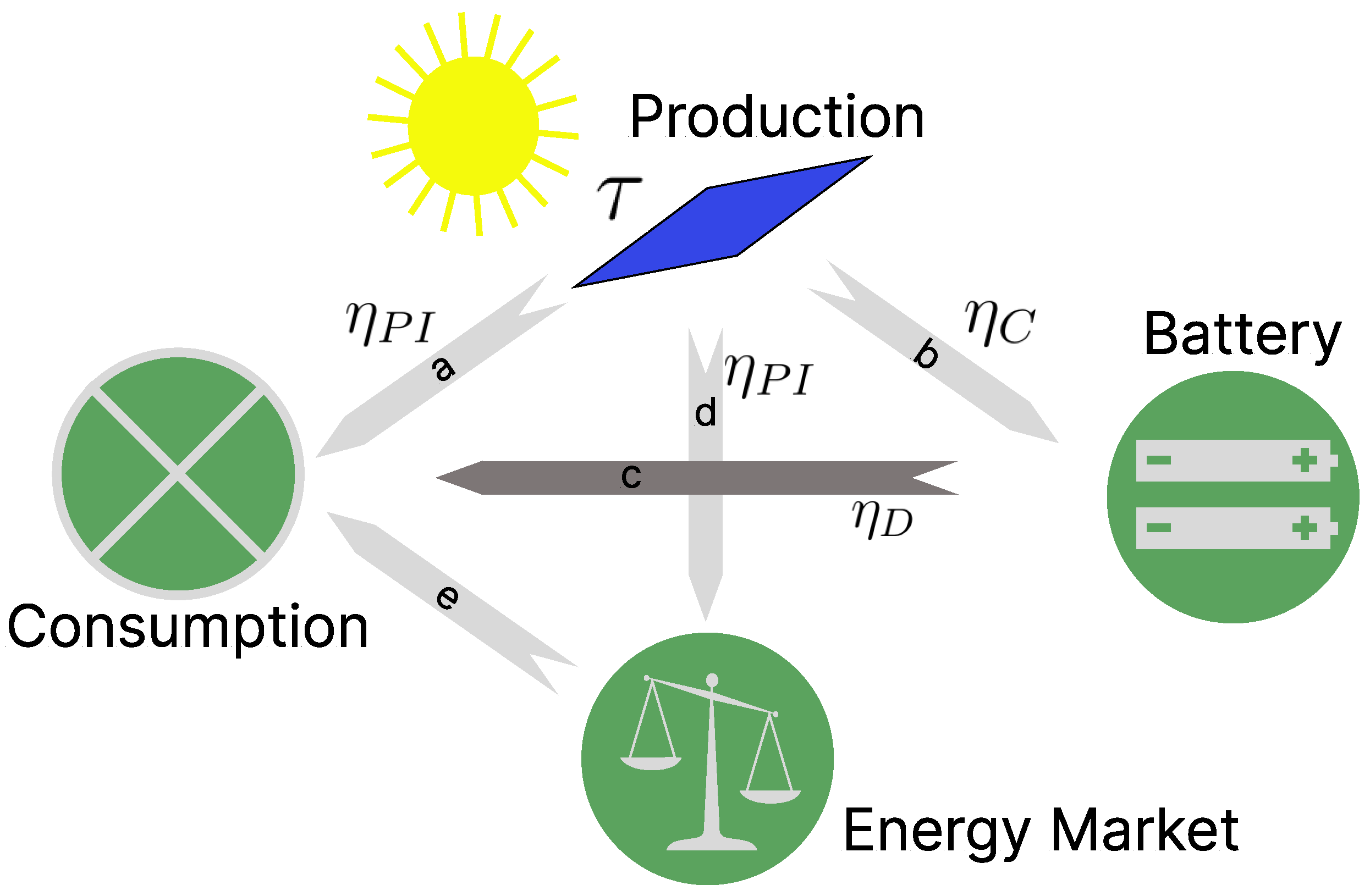
2.1. Production–Consumption Cycle

The production–consumption cycle is shown in Figure 1. PV modules convert electrical energy from the sun to DC electrical energy. The energy is either consumed, stored, or sold on the energy market. In case of underproduction, the energy demand is either satisfied from the battery or from the energy market. Detailed explanations of the paths (a)–(e) in Figure 1 are as follows:

(a)

When the production and load are balanced, the produced electricity is directly consumed. The produced DC electricity is converted by a power inverter to AC electricity. Here, we assume that the inversion has an efficiency of ${\eta }_{PI}=0.91$ [42].

(b)

When there is overproduction, the excess energy is stored in the battery until the maximum battery capacity is reached. The efficiency of charging the battery is assumed to be ${\eta }_C=0.95$ [42].

(c)

When there is underproduction, the energy demand is fulfilled by the battery first. In this case, we have two losses: one associated with discharging the battery and the other one associated with the power inverter. The total efficiency is assumed to be ${\eta }_D=0.9$ [42].

(d)

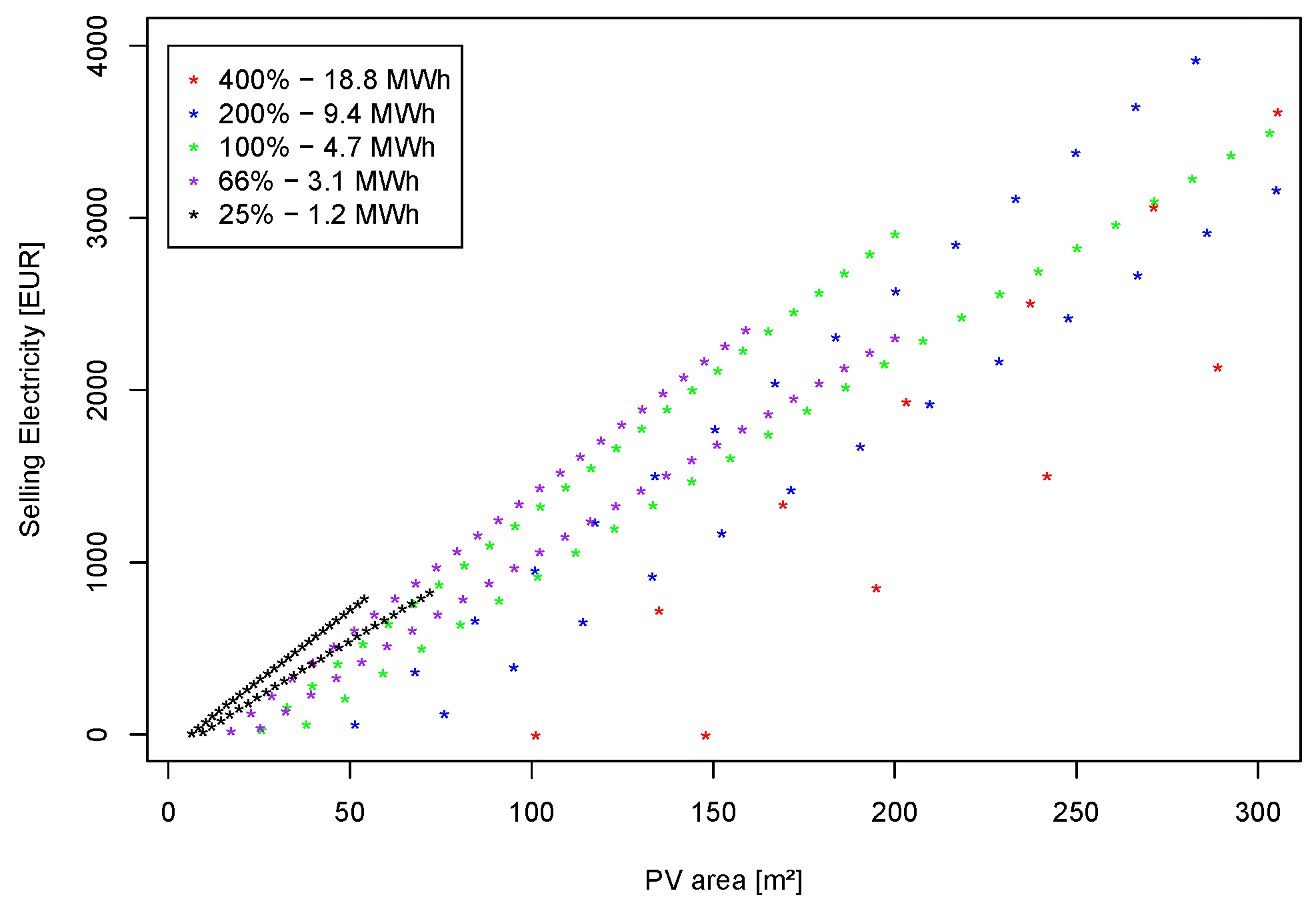
When there is overproduction and the battery is fully charged, the electricity can be transferred to the main grid and sold on the energy market with losses due to the power inverter, which has efficiency ${\eta }_{PI}=0.91$. The price received for each kWh sold is in Germany bounded by law currently at a price $p_{sell}=0.07$ EUR/kWh [43].

(e)

When there is underproduction and there is not enough energy in the battery, the electrical gap needs to be compensated for from the energy market. Currently, the price is approximately $p_{buy}=0.4$ EUR/kWh including taxes (for anticipated price evolution, we refer to [44]).

We use this setup to estimate how much PV area and battery capacity are necessary to avoid buying any electricity. That is, path (e) is excluded, so that no additional costs will arise in the future except for maintenance. This optimization is discussed in Section 3. To model the production of electricity, we use hourly solar radiation data from July 2002 to June 2022. The model for the hourly consumption is based on data from 2010. The data sets for production and consumption, and for the characteristics of the PV modules and the battery, are presented below.

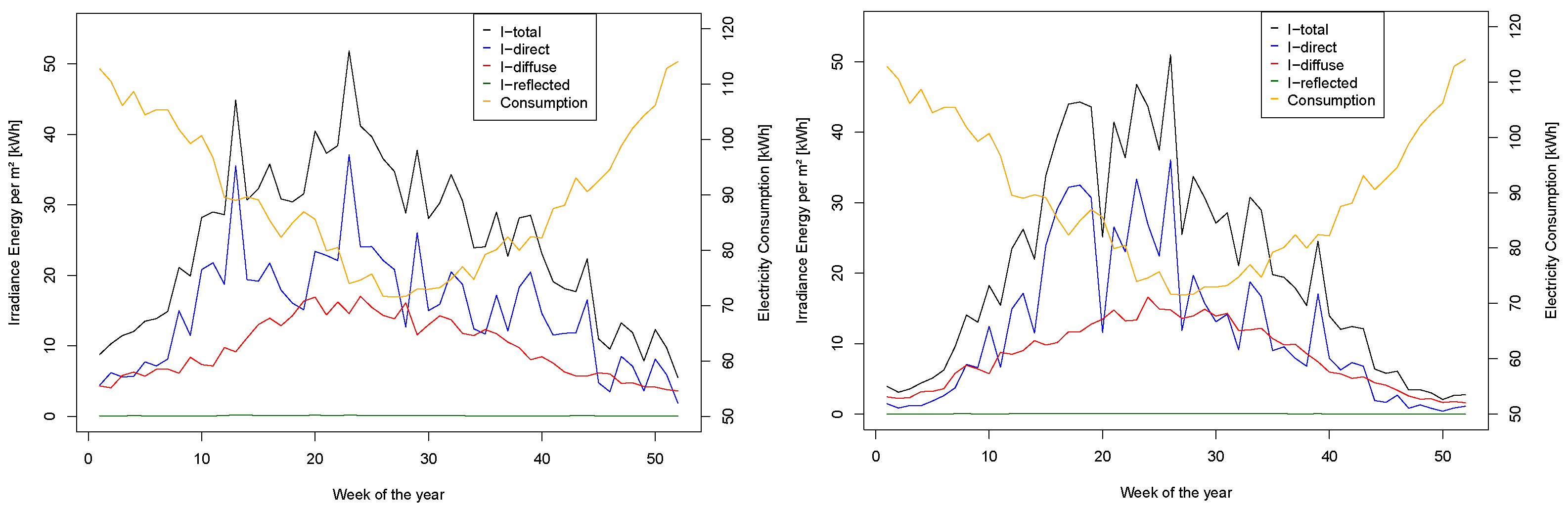
2.2. Production Data

In this paper, we are interested in the electrical energy that can be produced by PV modules from solar radiation. We calculate the electrical DC energy $E_{\mathrm{el},l}$ for different locations l as the integral over time of the total irradiance per square meter $I_{\mathrm{total},l,t}$, multiplied by the PV area P in m${}^2$, multiplied by the efficiency $\tau$ of the PV module. Benda and Černá [45] compared different PV modules and efficiencies. Based on their research, we choose $\tau =20\%$.

The electrical energy can therefore be expressed as

$$E_{\mathrm{el},l}=\tau P\int dt{I}_{\mathrm{total},l,t},$$

(1)

where

$$I_{\mathrm{total},l,t}=I_{\mathrm{direct},l,t}+I_{\mathrm{diffuse},l,t}+I_{\mathrm{reflected},l,t}.$$

(2)

The total irradiance consists of three parts. The direct irradiance $I_{\mathrm{direct},l,t}$ is the solar radiation that directly reaches the PV modules. Some of the solar radiation is scattered by clouds or by the particles of the Earth’s atmosphere. This is represented by the diffuse irradiance $I_{\mathrm{diffuse},l,t}$. Solar radiation that is reflected by the ground is represented by $I_{\mathrm{reflected},l,t}$. The three irradiances are described by

$$I_{\mathrm{direct},l,t}=\frac{\mathrm{FDIR}}{cos(\Theta )}cos\left(\gamma \right),$$

(3)

where $\Theta$ is the zenith angle of the sun and $\gamma$ is the angle between the normal vector of the PV module and the sun (see Figure 2). The total sky direct solar radiation at surface (FDIR) is the amount of direct solar radiation reaching the surface of the Earth in units of J/m${}^2$ (Joules per square meter). We obtain the FDIR from the ERA5 data [41] along with the data set for global horizontal irradiance (GHI) and the dimensionless albedo parameter $\alpha$ representing the Earth’s reflectivity. The GHI is the amount of solar radiation (also known as shortwave radiation) that reaches a horizontal plane at the surface of the Earth. This parameter comprises both direct and diffuse solar radiation and is in units of J/m${}^2$. All three data sets contain hourly data. The data for GHI and FDIR give the accumulated values for a period of 1 h ending at the relevant date and time. The data for albedo give the average albedo measure for that hour. Let the time t be the hour under consideration. The data are available on a grid with a $0.25$° resolution. We used the data covering an area surrounding Germany bounded by longitudes of 6° E and 15° E and latitudes of 47° N and 55° N, so in total, there are $33\times 37=1221$ grid cells of data.

From GHI and FDIR, we can extract the diffuse horizontal irradiance (DHI) by

$$\mathrm{DHI}=\mathrm{GHI}-\mathrm{FDIR}.$$

(4)

The diffuse irradiance can then be expressed as

$$I_{\mathrm{diffuse},l,t}=\mathrm{DHI}\frac{1+cos\left(\lambda \right)}{2},$$

(5)

where $\lambda$ is the installation angle of the PV module (see Figure 2). Mubarak et al. [46] suggest that PV modules should be oriented toward east and west, because then, there is a greater overlap between the time intervals of electricity production and demand. Therefore, we assume that our PV modules are positioned at an angle $\lambda =15$° toward east and west, each covering 50% of the total area. For other orientations, one can use their factors for different orientations as a first approximation.

Finally, we can express the reflected radiation as

$$I_{\mathrm{reflected},l,t}=\alpha \mathrm{GHI}\frac{1-cos\left(\lambda \right)}{2}.$$

(6)

As an example, the weekly irradiance values for one grid point are plotted in Figure 3 for the year 2021. The direct irradiance fluctuates strongly compared to the diffuse irradiance. The total irradiance is significantly higher in the summer than in the winter. The reflected irradiance is almost negligible, since the modules are located at an angle $\lambda =15$°, nearly flat on the ground, and hence, little of the radiation reflected by the ground reaches the PV modules.

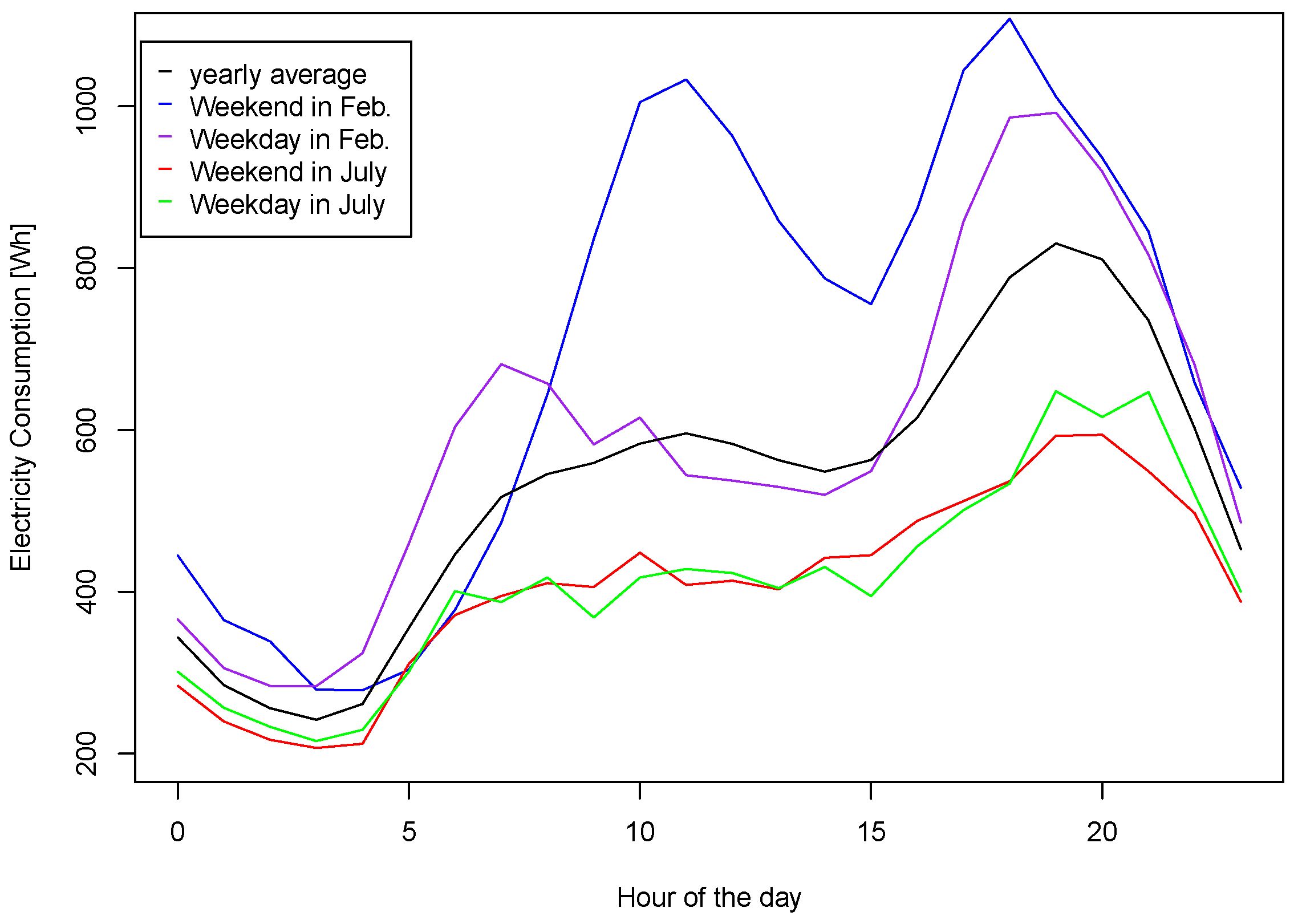
2.3. Consumption Data

We use consumption data from [40] that include electricity usage values on the second scale for 74 households in Berlin, Germany from 1 January 2010 to 31 December 2010. This data set has been used in other studies (e.g., [46,47]). We used the mean consumption of the 74 households, which is around $4.7$ MWh per year and is a good representation of a four-person household consumption curve in Germany [40]. Since our irradiance data are on an hourly scale, we accumulated the consumption data to an hourly scale (see Figure 4). The electricity usage is different from month to month but also depends on weekdays and the hour of the day. Two example days are plotted together with the total mean in Figure 4. It can be seen that the need for electricity is higher in the winter (February) compared to the summer (July). This higher consumption in the winter is underlined in Equation (11), which also shows the weekly consumption for one year. For information on the non-linear relationship between temperature and electricity consumption, we refer to [48].

Based on the hourly mean across 74 households in this data set, we model a time series for the hourly consumption with a quasi-Fourier series and temporal autoregressive model. Starting from Section 3.2, we also want to make conclusions for different yearly consumption levels. For example, for an annual consumption level of $3.2$ MWh, we multiply the consumption curve by $\frac{3.2}{4.7}$. In the following, we describe the consumption by the consumption rate C, which is the percentage of the default consumption level of $4.7$ MWh ($C=100\frac{3.2}{4.7}\%$ in this case).

2.4. Storage

Battery storage is an essential part of the setup for being self-sufficient and for the broader energy transition of society [49,50]. This is reflected in the large body of research in different directions, from the optimal economic usage of batteries (e.g., optimal charging cycles [51]), to making batteries cheaper and more robust (e.g., by using aluminum, sulfur, and salt as the main components; [52]). Hence, it is likely that battery prices will drop in the future, even though they currently remain high.

To gather information on current battery sizes and costs for private households, we collected information from $n=46$ companies in Germany that install PV modules combined with electricity storage in private households. The average storage price for an installed solution before tax was ${\overline{x}}_{\mathrm{sp}}=776$ EUR/kWh with a sample standard deviation of $s_{\mathrm{sp}}=10$ EUR/kWh. For private households in Germany, we have to consider an additional 19% value-added tax. The largest battery storage we were able to identify has a capacity of 1520 kWh [53], which consists of a 20 KWh electrical battery and a 1500 kWh hydrogen storage unit that is designed for use as seasonal storage (for details on seasonal storage, see [54]).

We obtain the yearly costs for the battery with the annuity equation. We assume that we take a loan of 100% of the battery costs $K_0$ and pay it back with a monthly constant rate $p_{\mathrm{MBC}}$ for $n=10$ years, which is the time of the warranty of the battery. The outstanding debt after n years is then given by

$$E_n=K_0{q}^n-\frac{p_{\mathrm{MBC}}(q^n-1)}{q-1},$$

(7)

where $q=p+1$. We assume it is possible to take out a loan at an interest rate of $p=3\%$ [55], so $q=1.03$. Then, we can calculate the yearly cost of the MBC $p_{\mathrm{MBC}}$ by setting $E_n=0$ (since we want to have zero debt at the end), yielding

$$p_{\mathrm{MBC}}=\frac{K_0{q}^n(q-1)}{q^n-1}=\frac{776\times 1.{03}^{10}\times 0.03}{1.{03}^{10}-1}=90.97\mathrm{EUR}/\mathrm{kWh}.$$

(8)

2.5. Photovoltaic Modules

Since solar energy is available for free in large quantities across the Earth, it is possible that the generation of electrical energy from PV modules will become humanity’s main source of energy in the future. Making this more likely is that prices for solar electricity continue to drop [9]. There is also a great deal of ongoing research into making PV modules cheaper, more efficient, and more sustainable in terms of production materials [10,56]. An important step in the future will be if communities can 3D print their own PV modules [57].

To gather information about the prices of PV modules today, we collected PV module prices $n=22$ from four online shops with a warranty of at least 15 years [58,59,60,61]. The average price for only the PV module excluding taxes is ${\overline{x}}_{\mathrm{PV}}=101$ EUR/m${}^2$ with $s_{\mathrm{PV}}=5.3$ EUR/m${}^2$. These modules have on average a rate output power of 402 kWp. Based on the interviews with the installation companies, it is further assumed that the installation costs are an additional 100% over the PV module prices. We also have to consider the additional 19% value-added tax. The total price per m${}^2$, including installation and taxes, is

$$P{V}_{{\mathrm{m}}^2}=240\mathrm{EUR}.$$

(9)

Again, we use the annuity equation and assume that we take out a 100% loan with interest rate $p=3\%$ and pay it back over the $n=15$ years of warranty at a constant rate. In that case, we can calculate the yearly costs of the PV per m${}^2$ as

$$p_{\mathrm{PV}}=\frac{K_0{q}^n(q-1)}{q^n-1}=\frac{240\times 1.{03}^{15}\times 0.03}{1.{03}^{15}-1}=20.1\mathrm{EUR}/\mathrm{m}{}^2$$

(10)

PV modules can also be characterized by their kWp. Based on our data, the price per kWp is $P{V}_{\mathrm{kWp}}=1394$ EUR including installation and tax.

In our model, we do not take the power reduction over time of the PV modules nor the battery into account. This effect could be incorporated into the model by scaling the PV area and battery capacity accordingly.

3. Methods

3.1. Modeling the Hourly Electricity Demand

Based on the data presented in Section 2.3, the hourly demand for electricity is dependent on the hour of the day, whether it is a weekday or weekend, and the season of the year. Therefore, we modeled the average hourly consumption $c\left(t\right)$ between 2 January 2010 and 23 December 2010 using Fourier series and by taking temporal lags into account. We constructed and estimated the frequencies and parameters from the data set. The resulting logarithmic models are as follows:

$$ln\left(c\left(t\right)\right)\equiv \tilde{c}\left(t\right)=\left\{\begin{array}{cc}{\beta }_{d0}+T_d+D_d+Y_d+W_d+{ϵ}_d\hfill & \mathrm{if}t\mathrm{is}\mathrm{on}\mathrm{a}\mathrm{weekday}\hfill \\ {\beta }_{e0}+T_e+D_e+Y_e+W_e+{ϵ}_e\hfill & \mathrm{if}t\mathrm{is}\mathrm{on}\mathrm{a}\mathrm{weekend},\hfill \end{array}\right.$$

(11)

where ${\beta }_{d0},\dots ,{\beta }_{d9}$ and ${\beta }_{e0},\dots ,{\beta }_{e11}$ are the regression coefficients of the weekday and weekend model, respectively (see

Table 1. Estimated values for the consumption model.

Parameter			Estimate	Std. Dev.	p-Value
Equation (11)—Weekday consumption
	Intercept	${\widehat{\beta }}_{d0}$	1.535	0.0518	<$2\times {10}^{-16}$
	Time Lag 1	${\widehat{\beta }}_{d1}$	0.638	0.0124	<$2\times {10}^{-16}$
	Time Lag 2	${\widehat{\beta }}_{d2}$	−0.138	0.0089	<$2\times {10}^{-16}$
	Time Lag 3	${\widehat{\beta }}_{d3}$	0.552	0.0108	<$2\times {10}^{-16}$
	Time Lag 4	${\widehat{\beta }}_{d4}$	−0.292	0.0120	<$2\times {10}^{-16}$
	Daily Variation 1	${\widehat{\beta }}_{d5}$	−0.081	0.0032	<$2\times {10}^{-16}$
	Daily Variation 2	${\widehat{\beta }}_{d6}$	−0.074	0.0032	<$2\times {10}^{-16}$
	Yearly Trend 1	${\widehat{\beta }}_{d7}$	0.014	0.0017	<$2\times {10}^{-16}$
	Yearly Trend 2	${\widehat{\beta }}_{d8}$	−0.090	0.0049	<$2\times {10}^{-16}$
	Interaction 1	${\widehat{\beta }}_{d9}$	−0.013	0.0024	$4.18\times {10}^{-8}$
Equation (11)—Weekend consumption
	Intercept	${\widehat{\beta }}_{e0}$	1.687	0.0577	<$2\times {10}^{-16}$
	Time Lag 1	${\widehat{\beta }}_{e1}$	0.671	0.0198	<$2\times {10}^{-16}$
	Time Lag 2	${\widehat{\beta }}_{e2}$	−0.069	0.0162	$2.29\times {10}^{-5}$
	Time Lag 3	${\widehat{\beta }}_{e3}$	0.129	0.0141	<$2\times {10}^{-16}$
	Daily Variation 1	${\widehat{\beta }}_{e4}$	−0.170	0.0060	<$2\times {10}^{-16}$
	Daily Variation 2	${\widehat{\beta }}_{e5}$	0.103	0.0063	<$2\times {10}^{-16}$
	Yearly Trend 1	${\widehat{\beta }}_{e6}$	0.015	0.0025	$5.07\times {10}^{-10}$
	Yearly Trend 2	${\widehat{\beta }}_{e7}$	0.051	0.0030	<$2\times {10}^{-16}$
	Interaction 1	${\widehat{\beta }}_{e8}$	−0.022	0.0035	$2.24\times {10}^{-10}$
	Interaction 2	${\widehat{\beta }}_{e9}$	−0.037	0.0043	<$2\times {10}^{-16}$
	Interaction 3	${\widehat{\beta }}_{e10}$	−0.040	0.0053	$3.05\times {10}^{-14}$
	Interaction 4	${\widehat{\beta }}_{e11}$	0.030	0.0080	$1.52\times {10}^{-4}$

). $T_d$ and $T_e$ are the autoregressive components, $D_d$ and $D_e$ are the daily variations, $Y_d$ and $Y_e$ are the yearly trends, $W_d$ and $W_e$ are the interactions between daily and yearly trend, and $ϵ$ is independent white noise. The autoregressive models are given by

$$T_d={\beta }_{d1}\tilde{c}(t-1)+{\beta }_{d2}\tilde{c}(t-2)+{\beta }_{d3}\tilde{c}(t-24)+{\beta }_{d4}\tilde{c}(t-25)$$

(12)

and

$$T_e={\beta }_{e1}\tilde{c}(t-1)+{\beta }_{e2}\tilde{c}(t-2)+{\beta }_{e3}\tilde{c}(t-25),$$

(13)

where the time lag always refers to the hours of the previous day of the same category (e.g., for the weekend model, if t is on a Saturday at 9:00 a.m., then $t-25$ refers 25 h before to the previous Sunday at 8:00 a.m.). Based on the residuals’ autocorrelation function and the partial autocorrelation function, we choose the time lags in a step-wise manner until the functions showed no autocorrelation in the residuals. The daily variations and yearly trends are modeled by

$$D_d={\beta }_{d5}sin\left(\frac{2\pi \tilde{t}}{d}\right)+{\beta }_{d6}sin\left(\frac{4\pi \tilde{t}}{d}\right),$$

(14)

$$D_e={\beta }_{e4}sin\left(\frac{2\pi \tilde{t}}{d}\right)+{\beta }_{e5}cos\left(\frac{4\pi \tilde{t}}{d}\right),$$

(15)

$$Y_d={\beta }_{d7}sin\left(\frac{2\pi \tilde{t}}{y_d}\right)+{\beta }_{d8}sin\left(\frac{\pi \tilde{t}}{y_d}\right),\mathrm{and}$$

(16)

$$Y_e={\beta }_{e6}sin\left(\frac{2\pi \tilde{t}}{y_e}\right)+{\beta }_{e7}cos\left(\frac{2\pi \tilde{t}}{y_e}\right),$$

(17)

where $d=24$ is the number of hours in a day and $y_{d,e}$ is the total number hours in the year, with $y_e=2\times 51\times 24=2448$ for weekends and $y_d=5\times 51\times 24=6120$ for weekdays in common years. In leap years, however, there is an additional 24 h depending on whether the additional day is a weekday or a weekend. The time t counts the hour of the year and the time $\tilde{t}$ counts the hours of each category ($\tilde{t}\in \{1,...,y_{d,e}\}$). Finally, we model the interaction of the daily and yearly tends as

$$W_d={\beta }_{d9}sin\left(\frac{4\pi \tilde{t}}{d}\right)cos\left(\frac{2\pi \tilde{t}}{y_d}\right),\mathrm{and}$$

(18)

$$\begin{array}{c}{W}_e={\beta }_{e8}sin\left(\frac{2\pi \tilde{t}}{d}\right)cos\left(\frac{2\pi \tilde{t}}{y_e}\right)+{\beta }_{e9}sin\left(\frac{4\pi \tilde{t}}{d}\right)cos\left(\frac{2\pi \tilde{t}}{y_e}\right)\hfill \\ \hfill \hspace{1em}\hspace{1em}\hspace{1em}\hspace{1em}\hspace{1em}\hspace{1em}\hspace{1em}\hspace{1em}\hspace{1em}\hspace{1em}+{\beta }_{e10}sin\left(\frac{4\pi \tilde{t}}{d}\right)sin\left(\frac{\pi \tilde{t}}{y_e}\right)+{\beta }_{e11}cos\left(\frac{4\pi \tilde{t}}{d}\right)sin\left(\frac{\pi \tilde{t}}{y_e}\right).\end{array}$$

(19)

Since during the 8 days between 24 December 2010 and 1 January 2010 there are outliers in the data, we kept the daily profiles equal to the data from 2010 regardless of the weekday.

The values estimated by a least-squares fit for the consumption model $\widehat{\beta }$ are shown in Table 1. Estimates for the residuals ${ϵ}_d$ and ${ϵ}_e$ can be found in

Table 2. Estimated values for the residuals of the consumption model.

Model	Residuals	Sample Mean	Sample Std. Dev.	Durbin-Watson (p-Value)
Weekday	${ϵ}_d$	$7.1\times {10}^{-18}$	${\sigma }_{{ϵ}_d}=0.09081$	2.0624 (0.9907)
Weekend	${ϵ}_e$	$2.6\times {10}^{-18}$	${\sigma }_{{ϵ}_e}=0.08568$	1.9716 (0.1871)

, which shows values for the sample standard deviations ${\sigma }_{{ϵ}_d}$ and ${\sigma }_{{ϵ}_d}$ as well as estimates and p-values for the Durbin–Watson test.

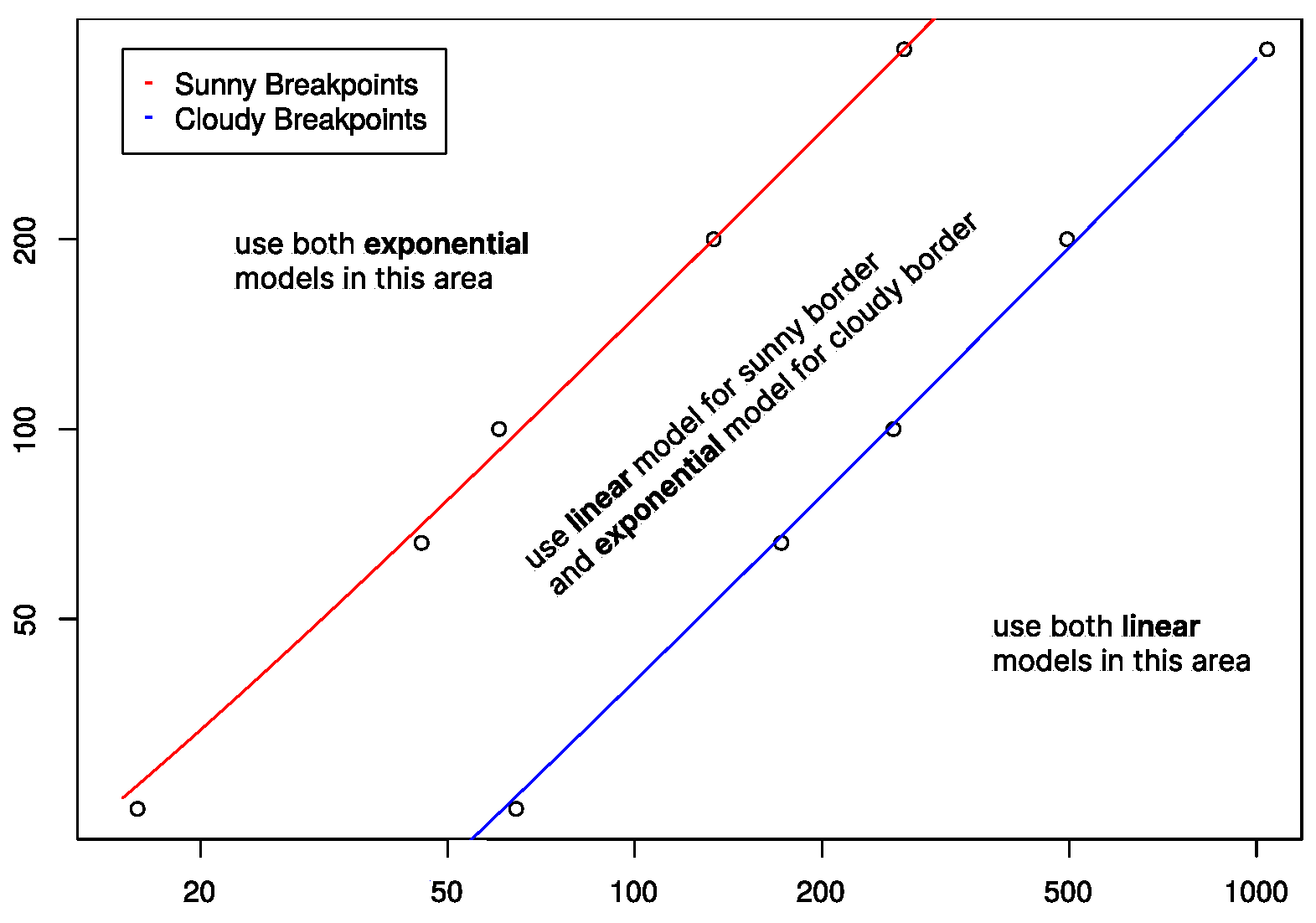
3.2. Optimization for PV Area and Battery Capacity

With the hourly production data and the hourly consumption model, we can evaluate the production–consumption cycle for one year for arbitrary values of the PV area and MBC. We evaluate a year from July in one year to June in the following year to avoid a break in the critical time period between November and February, during which consumption is high and production is low (see Figure 3).

We evaluate each year individually, so that we can say which years have greater requirements for the PV area and MBC. The annual evaluation also avoids compensating a “bad” year with the energy excess from a previous “good” year. Figure 5 shows the dependence of the amount of electricity that needs to be purchased on the PV area and the MBC for the year from July 2020 and June 2021 in the “cloudy” region (for the definition of this region, see Section 4).

It can be seen that it is possible to reach zero (i.e., no energy had to be bought throughout the year) for different configurations of PV area and MBC. In these cases, we are self-sufficient during that year. The important question we want to answer is: what is the minimal PV area that is necessary to be self-sufficient? This is because the PV area is the most common limiting factor for private households in Germany. We also want to understand the relationship between the MBC and the PV area P in different locations l in Germany and also for different electricity consumption rates C.

Therefore, we express the hourly battery load $B_{l,t}(P,C)$ for every hour of the year $t\in \{1,...,24\times 365(366\left)\right\}$ in the location l as follows

$$B_{l,t}(P,C)=\left\{\begin{array}{cc}max(B_{l,t-1}(P,C)+\frac{{\eta }_D}{{\eta }_{PI}}{\Delta }_{l,t}(P,C),0)\hfill & \mathrm{if}{\Delta }_{l,t}(P,C)<0\hfill \\ min(B_{l,t-1}(P,C)+\frac{{\eta }_C}{{\eta }_{PI}}{\Delta }_{l,t}(P,C),\mathrm{MBC})\hfill & \mathrm{if}{\Delta }_{l,t}(P,C)>0.\hfill \end{array}\right.$$

(20)

The hourly battery level is determined by the battery level from the previous hour and the difference in production and consumption over that hour (${\Delta }_{l,t}(P,C)=P{\eta }_{PI}\tau I_{\mathrm{total},l,t}-Cc\left(t\right)$). Since there are two different efficiencies related to charging and discharging the battery, we take this into account in the two cases for $B_{l,t}(P,C)$, whether ${\Delta }_{l,t}(P,C)$ is smaller or larger than zero. The hourly battery load cannot be negative and cannot exceed the maximum battery capacity. If $B_{l,t}(P,C)$ becomes smaller than zero in one hour, we set it to zero and have to buy the unmet energy demand from the energy market. On the other hand, if $B_{l,t}(P,C)$ exceeds MBC, we set it to MBC and can sell the excess energy in the energy market. So, we can see that the hourly battery load depends on how we choose the MBC.

Now, we can formulate an optimization problem to find the minimal required MBC for a given P, a given C, and in different locations l, under the condition that we do not have to buy any energy:

$$\begin{array}{c}\hfill \begin{array}{cc}\hfill & \mathrm{Minimize}\mathrm{MBC}\hfill \\ & \mathrm{subject}\mathrm{to}{B}_{l,t-1}(P,C)+\frac{{\eta }_D}{{\eta }_{PI}}{\Delta }_{l,t}(P,C)\ge 0,\mathrm{for}\mathrm{all}t\hfill \\ & B_{l,0}(P,C)=10,\mathrm{for}\mathrm{all}l,P,C.\hfill \end{array}\end{array}$$

Since the solution depends on l, P, and C, we denote the optimum by MBC${}_l(P,C)$. Note that $B_{l,t}(P,C)$ depends on the upper bound MBC according to Equation (20). We run the optimization on the data of each year between July and June, assuming that we start with an initial battery load of $B_{l,0}(P,C)=10$ kWh. We perform the optimization by bisection with the convergence criterion that the distance between the least known upper bound and the greatest known lower bound is less than $0.01$ kWh. All code and data to reproduce the analysis are available open-source data (see data availability statement).

In the case that the PV area is too small to provide the required energy, there is no solution for this optimization problem. Hence, we can optimize for the minimal required PV area $P_{min,l}\left(C\right)$ in different locations around Germany:

$$\begin{array}{c}\hfill \begin{array}{cc}\hfill & \mathrm{Minimize}P\hfill \\ & \mathrm{subject}\mathrm{to}{B}_{l,t-1}(P,C)+\frac{{\eta }_D}{{\eta }_{PI}}{\Delta }_{l,t}(P,C)\ge 0,\mathrm{for}\mathrm{all}t\hfill \\ & B_{l,0}(P,C)=5,\mathrm{for}\mathrm{all}l,P,C.\hfill \end{array}\end{array}$$

We performed this optimization using the bisection method under the convergence criterion that the distance between the least known upper bound and the greatest known lower bound is less than $0.01$ m${}^2$.

We determined $P_{min,l}\left(C\right)$ for each grid cell and for each of the 20 years individually. By doing so, we can rule out that energy surplus from one year is carried forward into a “bad” year. The minimal PV area for each grid cell for the default consumption rate of $C=100\%$ for the worst year is plotted in Figure 6.

In Figure 7, we plotted the relationship between MBC${}_l(P,C)$ and PV area for different values of PV area, different consumption rates, and in two representative locations (“cloudy” and “sunny”).

For a conservative estimation of the required MBC${}_l(P,C)$ for a given PV area and a given C, we have to consider the uncertainty of the consumption model $c\left(t\right)$. We can cover the small variance by adding the “worst” 3-$\sigma$-interval offset of the uncertainties to the MBC ${\delta }_{MBC}\left(C\right)$ (like a backup battery) with the uncertainties from Table 2,

$${\delta }_{\mathrm{MBC}}\left(C\right)=C\frac{{\eta }_D}{{\eta }_{PI}}exp(3max({\sigma }_{{ϵ}_d},{\sigma }_{{ϵ}_e})max\left(c\left(t\right)\right)=1.659C\mathrm{kWh}.$$

(21)

The factor of $\frac{{\eta }_D}{{\eta }_{PI}}$ is due to the uncertainty linearly affecting the condition of the constraint (see [62]). The 3-$\sigma$ uncertainty covers $99.5\%$ of regular daily routines, such as boiling water, cooking, or watching TV at variable times, because these daily routines are covered in the consumption curve and the excess use in one hour will be compensated in the next hour. However, it does not cover larger, outlier events such as celebrating a 30th birthday at home with many guests, cooking, loud music, and special lightning in January. Such events with large electricity demand are probably not compensated within the next or previous hours. Hence, if we wanted to take into account such events, this could be completed by either including these energy demands in the consumption curve or increasing the MBC by the energy needed for such events, especially if these events take place in the time period between November and February.

One final assumption we are making is that the coverage of $99.5\%$ will be extended by the behavior of the household itself. If the household has some kind of feedback on the level of battery load, this knowledge will affect their behavior, resulting in lower electricity use at critical times.

4. Results

We calculate the minimal resources $P_{\min ,l}\left(C\right)$ and MBC${}_l(P,C)$ required to achieve 100% self-sufficiency in each of the past 20 years and in each of the 1221 grid cells for different consumption rates. We plot, for every grid cell, $P_{min,l}$ for the worst year in Figure 6 for the default consumption rate $C=100\%$. The red crosses in the map indicate the grid cell where the highest ($38.7$ m${}^2$) and lowest ($24.8$ m${}^2$) PV area is necessary. As expected, in the south, the required PV area is smaller than in the north. We select these two representative locations with the highest and lowest PV requirements to set upper and lower limits. This allows us to make statements that apply to the whole of Germany. We call these two locations “sunny” and “cloudy”.

Figure 7 shows the MBC${}_l(P,C)$ that is needed to gain 100% electrical self-sufficiency, depending on the PV area that is available, the consumption rate C, and for the “sunny” and “cloudy” location. As expected, when less electricity is required, the required PV area and MBC are smaller and vice versa. We can then estimate the relationship between MBC and PV area. In Figure 7, it can be seen that there is a break in each lower (sunny location) and upper (cloudy location) plot. For PV areas smaller than the breakpoint, the gradient of MBC${}_l(P,C)$ is exponential with increasing PV area. The gradient of MBC${}_l(P,C)$ is linear for PV areas larger than the breakpoint. The breakpoints are obtained manually from the data and plotted in Figure 8. In the following, we will only consider the “sunny” and “cloudy” locations. Therefore, we write MBC${}_s(P,C)$ and MBC${}_c(P,C)$ for these two locations, respectively.

Based on Figure 8, we can conclude from the consumption level and the PV area that we have available (we should use as much PV area as possible, since the PV area is cheap compared to the battery costs) which models we should choose to describe the relationship between MBC${}_s(P,C)$, MBC${}_c(P,C)$ and PV area. The four models for cloudy and sunny, each with a linear and an exponential model, are chosen as follows:

$${\mathrm{MBC}}_{s,\mathrm{lin}}(P,C)={\gamma }_{sl,0}+{\gamma }_{sl,1}C+{\gamma }_{sl,2}P+{ϵ}_{sl},$$

(22)

$${\mathrm{MBC}}_{c,\mathrm{lin}}(P,C)={\gamma }_{cl,0}+{\gamma }_{cl,1}C+{\gamma }_{cl,2}P+{ϵ}_{cl},$$

(23)

$$ln\left({\mathrm{MBC}}_{s,\exp }(P,C)\right)={\gamma }_{se,0}+{\gamma }_{se,1}C+{\gamma }_{se,2}P/C+{ϵ}_{se},$$

(24)

and

$$ln\left(MB{C}_{c,\exp }(P,C)\right)={\gamma }_{ce,0}+{\gamma }_{ce,1}C+{\gamma }_{ce,2}P/C+{ϵ}_{ce}.$$

(25)

The estimated parameters can be found in

Table 3. Estimated values for the relationship between MBC and PV area.

Parameter			Estimate	Std. Dev.	p-Value
Equation (22)—MBC, sunny, linear
	Intercept	${\widehat{\gamma }}_{sl,0}$	2.996	1.6274	0.069
	Linear Consumption	${\widehat{\gamma }}_{sl,1}$	0.843	0.0186	<$2\times {10}^{-16}$
	Linear PV area	${\widehat{\gamma }}_{sl,2}$	−0.327	0.0122	<$2\times {10}^{-16}$
Equation (23)—MBC, cloudy, linear
	Intercept	${\widehat{\gamma }}_{cl,0}$	0.330	1.7815	0.854
	Linear Consumption	${\widehat{\gamma }}_{cl,1}$	1.014	0.0640	$3.42\times {10}^{-15}$
	Linear PV area	${\widehat{\gamma }}_{cl,2}$	−0.177	0.0224	$1.69\times {10}^{-8}$
Equation (24)—MBC, sunny, exponential
	Intercept	${\widehat{\gamma }}_{se,0}$	7.209	0.3564	<$2\times {10}^{-16}$
	Exp. Consumption	${\widehat{\gamma }}_{se,1}$	0.007	0.0007	$2.91\times {10}^{-10}$
	Exp. PV/C	${\widehat{\gamma }}_{se,2}$	−5.825	0.6157	$9.71\times {10}^{-10}$
Equation (25)—MBC, cloudy, exponential
	Intercept	${\widehat{\gamma }}_{ce,0}$	6.773	0.0940	<$2\times {10}^{-16}$
	Exp. Consumption	${\widehat{\gamma }}_{ce,1}$	0.007	0.0003	<$2\times {10}^{-16}$
	Exp. PV/C	${\widehat{\gamma }}_{ce,2}$	−1.460	0.0514	<$2\times {10}^{-16}$

. Based on these relations, we can estimate the costs for self-sufficiency, as discussed below.

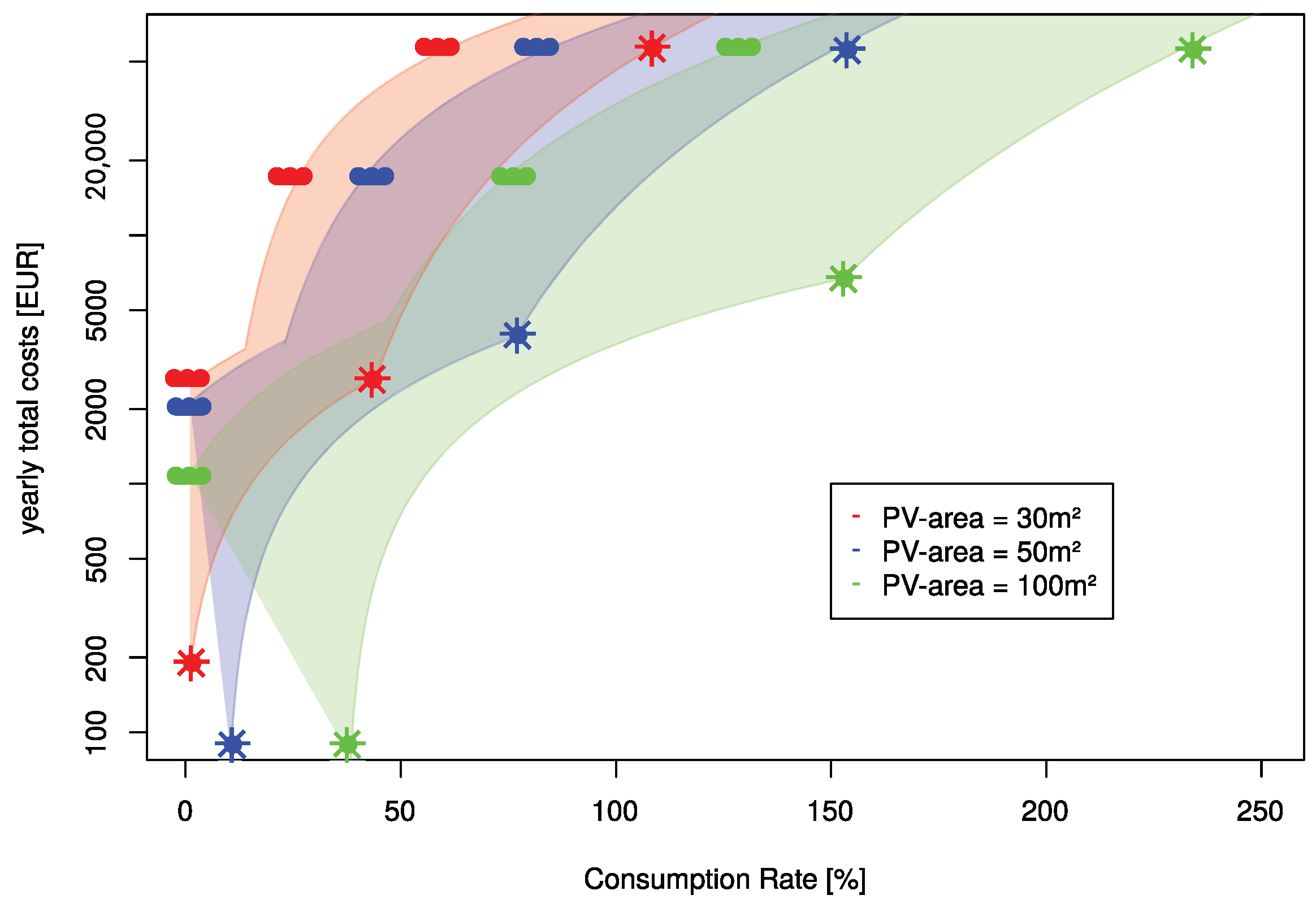
Costs for Solar Self-Sufficiency

The total price $Q_l$ per year at different locations l includes the annual price that one has to pay for the setup of the battery and PV area $p_A$ and is reduced by the amount of electricity $g_{\mathrm{el}}$ that one can sell on the market within the year and also by the default price $g_d$ of the electricity that one would have paid without the setup. Hence, $Q_l$ contains only the additional costs

$$Q_l=p_A({\mathrm{MBC}}_l(P,C),P,p_{\mathrm{MBC}},p_{\mathrm{PV}})-g_{\mathrm{el}}(l,P,C,p_{\mathrm{sell}})-g_d(C,p_{\mathrm{buy}})$$

(26)

We now look into each of these components individually. The default price for electricity $g_d$ is the amount of electricity consumed times the price for each kWh $p_{\mathrm{buy}}$. To model $g_{\mathrm{el}}$, we plot the annual energy sold against the PV area in Figure 9 and find a linear relationship in both the sunny ($g_{\mathrm{el},s}$) and the cloudy ($g_{\mathrm{el},c}$) region. Based on this plot, we estimate that

$$g_{\mathrm{el},s}(P,C)={\gamma }_{\mathrm{el},s,0}+{\gamma }_{\mathrm{el},s,1}P+{\gamma }_{\mathrm{el},s,2}C+{ϵ}_{\mathrm{el},s}$$

(27)

and

$$g_{\mathrm{el},c}(P,C)={\gamma }_{\mathrm{el},c,0}+{\gamma }_{\mathrm{el},c,1}P+{\gamma }_{\mathrm{el},c,2}C+{ϵ}_{\mathrm{el},c}.$$

(28)

The estimated parameters can be found in

Table 4. Estimated values for the relationship between the amount of money gained from selling surplus electricity, the consumption rate, and the PV area.

Parameter			Estimate	Std. Dev.	p-Value
Equation (27)—Selling, sunny
	Intercept	${\widehat{\gamma }}_{\mathrm{el},s,0}$	−32.800	9.8304	0.00111
	PV area	${\widehat{\gamma }}_{\mathrm{el},s,1}$	16.217	0.0491	<$2\times {10}^{-16}$
	Consumption	${\widehat{\gamma }}_{\mathrm{el},s,2}$	−3.410	0.0819	<$2\times {10}^{-16}$
Equation (28)—Selling, cloudy
	Intercept	${\widehat{\gamma }}_{\mathrm{el},c,0}$	−37.625	11.6773	0.00162
	PV area	${\widehat{\gamma }}_{\mathrm{el},c,1}$	12.820	0.0439	<$2\times {10}^{-16}$
	Consumption	${\widehat{\gamma }}_{\mathrm{el},c,2}$	−3.839	0.0959	<$2\times {10}^{-16}$

. In the following, we model the setup cost $p_A$ by separating it into the total costs for the MBC ($Q_{\mathrm{MBC}}$) and the total costs for the PV area ($Q_{\mathrm{PV}}$),

$$p_A({\mathrm{MBC}}_l(P,C),P,p_{\mathrm{MBC}},p_{\mathrm{PV}},C)=Q_{\mathrm{MBC}}({\mathrm{MBC}}_l(P,C),p_{\mathrm{MBC}})+Q_{\mathrm{PV}}(P,p_{\mathrm{PV}}),$$

(29)

where the total yearly cost for the PV area is the PV area multiplied by the yearly price per m${}^2$,

$$Q_{\mathrm{PV}}(P,p_{\mathrm{PV}})=P{p}_{\mathrm{PV}},$$

(30)

and the costs for the battery are the MBC multiplied by the yearly costs per kWh $p_{MBC}$. We derived the relationship between MBC and PV area above, so we have

$$Q_{\mathrm{MBC}}({\mathrm{MBC}}_l(P,C),p_{\mathrm{MBC}})=p_{\mathrm{MBC}}{\mathrm{MBC}}_l(P,C).$$

(31)

With these equations, we have derived all contributors to the total price for self-sufficiency $Q_l$. The total prices for self-sufficiency by the PV area and the consumption rate for the sunny and cloudy limits are plotted in Figure 10 and Figure 11.

From Figure 10, one can see that a larger PV area decreases the total cost of self-sufficiency in any location in Germany. In contrast, a higher consumption of electricity yields to greater yearly costs (see Figure 11). It can also be seen that being self-sufficient can possibly result in financial benefits if the consumption level is low and there is a large PV area. Both of these factors reduce the need for a large, expensive battery. However, the cheaper approach makes more sense in sunnier regions, which are located primarily in the south of Germany.

Using Figure 10 and Figure 11 in addition to Equation (26) lets one estimate the requirements and the expected annual cost for solar self-sufficiency. It is worth noting that with a higher consumption of electricity, for example, by an electric car or a heat pump, it is still possible to achieve solar self-sufficiency, but large PV areas and high MBCs are necessary. One can optimize the costs by taking into account that it is not only important how much electricity is needed but also when it is needed [46,63].

5. Discussion and Conclusions

In this paper, we modeled the hourly annual electricity demand of an average four-person household using Fourier series and an autoregressive statistical model. We applied the results to the time period from July 2002 to June 2022. The consumption model was compared to hourly solar radiation data from ERA5. From the comparison of these values, we optimized how much PV area and how much battery capacity would have been necessary for electricity self-sufficiency during these 20 years. The values were determined for a fixed, optimal orientation of the solar modules with a 15° inclination toward east and west for 1221 grid cells in and around Germany. From the grid cells located within Germany, the two cells with the highest and lowest demand of PV area were then selected as representatives for all of Germany and designated as “cloudy” and “sunny”.

For the cloudy and sunny regions, the relationship between battery capacity and PV area was estimated for different electricity consumption rates. We also derived the expected annual cost of self-sufficiency from the models. Our model shows that using more PV area for self-sufficiency is cheaper. This is particularly interesting given that currently, 89% of suitable rooftop space is still vacant [8]. In addition, our model shows that if the annual electricity consumption is low, combined with a sufficiently large solar area, it may be possible to earn money by selling surplus electricity in sunny regions while being self-sufficient. To reduce costs for self-sufficiency, the main advice is to reduce one’s electricity consumption and/or to move the consumption to sunny hours of the day, if possible [46].

Using this model, people interested in living self-sufficiently can estimate which conditions have to be fulfilled and what costs can be expected. In particular, our model shows that self-sufficient households can be built with today’s storage technology (1520 kWh Hydrogen Storage [53]). In providing this information, we aim to lower the barrier for private households to achieve self-sufficiency. This could help support a bottom–up sustainability transformation to achieve the SDGs “take urgent action to combat climate change and its impacts” [1] and “ensure access to affordable, reliable, sustainable and modern energy for all” [2]. In the future, we expect households and communities to become more interested in solar self-sufficiency as the prices of PV systems and batteries continue to decline in the coming years.

Our model is characterized by the following facts. First, it allows to optimize for 100% self-sufficiency. We explicitly do not say that this is economically the best way, but everyone can at least have an idea on the dimensions of required tools and the expected costs. Second, we evaluate with our model the difference between electricity consumption and production on an hourly basis to provide a more reliable result compared to weekly or daily evaluation. Third, the model is based on solar radiation data from ERA5, which are available worldwide. Thus, it can be easily transferred to another area using the provided open source code. Fourth, we built our model based on historical data without future forecasts, which would induce further uncertainty in the provided information (e.g., required storage capacity at each location). In turn, this means that only influences of climate change and global warming from the past are included in the model. Nevertheless, forecasting the input quantities to obtain reliable predictions of the requirements/costs for 100% self-sufficiency is an important field for future research.

The impact of climate change and global warming on the model can be mainly due to more frequent weather extremes [64]. The critical period for self-sufficiency is between November and February, as less electricity is produced and more electricity is consumed during this time. Weather extremes can shorten or lengthen this critical period and thus the requirements for self-sufficiency by providing more or less sunny and warm days within this period.

In future work, we will further elaborate on the weaknesses of our models. These include (1) adding more consumption curves with different profiles (e.g., those in [65]), (2) adding more past radiation data to make the self-sufficiency conditions more stable, (3) modeling the radiation data on a minute-by-minute frequency to reduce the error in the comparison of the aggregated consumption data, (4) taking into account the battery life, as well as the degradation of the battery and the PV modules over time, (5) considering the effects of temperature on the efficiency of the PV modules, and (6) considering different positions and orientation angles of the PV modules.

Another possible research avenue would be to take the idea of self-sufficiency further and find and model solutions for complete self-sufficiency, including water treatment and food cultivation [66]. Modeling the combination of residential solar and wind energy would be another interesting research topic, following [67]. Another possibility could be to extend our approach to the SDG “make cities and human settlements inclusive, safe, resilient and sustainable” [68] by connecting self-sufficient single-family homes into communities to form self-sufficient smart villages.

References

1. United Nations. Goal 13|Take Urgent Action to Combat Climate Change and Its Impacts; United Nations: New York, NY, USA, 2015. [Google Scholar]
2. United Nations. Goal 7|Ensure Access to Affordable, Reliable, Sustainable and Modern Energy for All; United Nations: New York, NY, USA, 2015. [Google Scholar]
3. Panda, B. Top down or bottom up? A study of grassroots NGOs’ approach. J. Health Manag. 2007, 9, 257–273. [Google Scholar] [CrossRef]
4. Lotz, H. Technical and Political Regulations for a CFC Phaseout. Massgaben aus Technik und Politik für den FCKW-Ausstieg; U.S. Department of Energy, Office of Scientific and Technical Information: Oak Ridge, TN, USA, 1990.
5. Pawlik, V. Anzahl der Veganer in Deutschland 2015–2022. 2022. Available online: https://de.statista.com/statistik/daten/studie/445155/umfrage/umfrage-in-deutschland-zur-anzahl-der-veganer/ (accessed on 10 October 2022).
6. Bundesamt, S. Upward Trend for Meat Substitutes Continued: Production Increased by 17% in 2021 Year on Year. 2022. Available online: https://www.destatis.de/EN/Press/2022/05/PE22_N025_42.html (accessed on 22 December 2022).
7. Frenette, E.; Bahn, O.; Vaillancourt, K. Meat, dairy and climate change: Assessing the long-term mitigation potential of alternative agri-food consumption patterns in Canada. Environ. Model. Assess. 2017, 22, 1–16. [Google Scholar] [CrossRef]
8. Kampwirth, R.; Ammon, M. Report: Solar-Häuser können Zehn Kohlekraftwerke Ersetzen-engl.: Solar houses can replace ten coal-fired power plants. 2022. Available online: https://www.presseportal.de/pm/22265/5259636 (accessed on 22 December 2022).
9. Kost, C.; Shammugam, S.; Fluri, V.; Peper, D.; Davoodi Memar, A.; Schlegl, T. Stromgestehungskosten Erneuerbare Energien; Fraunhofer-Institut für Solare Energiesysteme ISE: Freiburg, Germany, 2021. [Google Scholar]
10. Yang, C.; Zhang, S.; Hou, J. Low-cost and efficient organic solar cells based on polythiophene-and poly (thiophene vinylene)-related donors: Photovoltaics: Special Issue Dedicated to Professor Yongfang Li. Aggregate 2022, 3, e111. [Google Scholar] [CrossRef]
11. The Economist. Why Energy Insecurity Is Here to Stay. 2022. Available online: https://godfreytimes.com/2022/03/26/why-energy-insecurity-is-here-to-stay/ (accessed on 5 September 2022).
12. Alves, B. Germany: Monthly Electricity Prices 2022. 2022. Available online: https://www.statista.com/statistics/1267541/germany-monthly-wholesale-electricity-price/ (accessed on 5 September 2022).
13. Breyer, C.; Khalili, S.; Bogdanov, D.; Ram, M.; Oyewo, A.S.; Aghahosseini, A.; Gulagi, A.; Solomon, A.; Keiner, D.; Lopez, G.; et al. On the History and Future of 100% Renewable Energy Systems Research. IEEE Access 2022, 10, 78176–78218. [Google Scholar] [CrossRef]
14. Paulsen, K.; Hensel, F. Design of an autarkic water and energy supply driven by renewable energy using commercially available components. Desalination 2007, 203, 455–462. [Google Scholar] [CrossRef]
15. Müller, M.O.; Stämpfli, A.; Dold, U.; Hammer, T. Energy autarky: A conceptual framework for sustainable regional development. Energy Policy 2011, 39, 5800–5810. [Google Scholar] [CrossRef]
16. Schmidt, J.; Schönhart, M.; Biberacher, M.; Guggenberger, T.; Hausl, S.; Kalt, G.; Leduc, S.; Schardinger, I.; Schmid, E. Regional energy autarky: Potentials, costs and consequences for an Austrian region. Energy Policy 2012, 47, 211–221. [Google Scholar] [CrossRef]
17. Moss, T.; Francesch-Huidobro, M. Realigning the electric city. Legacies of energy autarky in Berlin and Hong Kong. Energy Res. Soc. Sci. 2016, 11, 225–236. [Google Scholar] [CrossRef]
18. Petrakopoulou, F.; Robinson, A.; Loizidou, M. Simulation and evaluation of a hybrid concentrating-solar and wind power plant for energy autonomy on islands. Renew. Energy 2016, 96, 863–871. [Google Scholar] [CrossRef]
19. Juntunen, J.K.; Martiskainen, M. Improving understanding of energy autonomy: A systematic review. Renew. Sustain. Energy Rev. 2021, 141, 110797. [Google Scholar] [CrossRef]
20. Engelken, M.; Römer, B.; Drescher, M.; Welpe, I. Transforming the energy system: Why municipalities strive for energy self-sufficiency. Energy Policy 2016, 98, 365–377. [Google Scholar] [CrossRef]
21. Ram, M.; Gulagi, A.; Aghahosseini, A.; Bogdanov, D.; Breyer, C. Energy transition in megacities towards 100% renewable energy: A case for Delhi. Renew. Energy 2022, 195, 578–589. [Google Scholar] [CrossRef]
22. Oyewo, A.S.; Aghahosseini, A.; Ram, M.; Lohrmann, A.; Breyer, C. Pathway towards achieving 100% renewable electricity by 2050 for South Africa. Sol. Energy 2019, 191, 549–565. [Google Scholar] [CrossRef]
23. Shin, H.; Geem, Z.W. Optimal design of a residential photovoltaic renewable system in South Korea. Appl. Sci. 2019, 9, 1138. [Google Scholar] [CrossRef]
24. Arcos-Vargas, A.; Cansino, J.M.; Román-Collado, R. Economic and environmental analysis of a residential PV system: A profitable contribution to the Paris agreement. Renew. Sustain. Energy Rev. 2018, 94, 1024–1035. [Google Scholar] [CrossRef]
25. Keiner, D.; Ram, M.; Barbosa, L.D.S.N.S.; Bogdanov, D.; Breyer, C. Cost optimal self-consumption of PV prosumers with stationary batteries, heat pumps, thermal energy storage and electric vehicles across the world up to 2050. Sol. Energy 2019, 185, 406–423. [Google Scholar] [CrossRef]
26. Ballesteros-Gallardo, J.A.; Arcos-Vargas, A.; Núñez, F. Optimal Design Model for a Residential PV Storage System an Application to the Spanish Case. Sustainability 2021, 13, 575. [Google Scholar] [CrossRef]
27. Jurasz, J.K.; Dabek, P.B.; Campana, P.E. Can a city reach energy self-sufficiency by means of rooftop photovoltaics? Case study from Poland. J. Clean. Prod. 2020, 245, 118813. [Google Scholar] [CrossRef]
28. Mutani, G.; Todeschi, V. Optimization of costs and self-sufficiency for roof integrated photovoltaic technologies on residential buildings. Energies 2021, 14, 4018. [Google Scholar] [CrossRef]
29. Lokar, J.; Virtič, P. The potential for integration of hydrogen for complete energy self-sufficiency in residential buildings with photovoltaic and battery storage systems. Int. J. Hydrogen Energy 2020, 45, 34566–34578. [Google Scholar] [CrossRef]
30. Hassan, Q.; Pawela, B.; Hasan, A.; Jaszczur, M. Optimization of Large-Scale Battery Storage Capacity in Conjunction with Photovoltaic Systems for Maximum Self-Sustainability. Energies 2022, 15, 3845. [Google Scholar] [CrossRef]
31. Colmenar-Santos, A.; Campíñez-Romero, S.; Pérez-Molina, C.; Castro-Gil, M. Profitability analysis of grid-connected photovoltaic facilities for household electricity self-sufficiency. Energy Policy 2012, 51, 749–764. [Google Scholar] [CrossRef]
32. Ecker, F.; Spada, H.; Hahnel, U.J. Independence without control: Autarky outperforms autonomy benefits in the adoption of private energy storage systems. Energy Policy 2018, 122, 214–228. [Google Scholar] [CrossRef]
33. Lund, P. Optimization of stand-alone photovoltaic systems with hydrogen storage for total energy self-sufficiency. Int. J. Hydrogen Energy 1991, 16, 735–740. [Google Scholar] [CrossRef]
34. Stahl, W.; Voss, K.; Goetzberger, A. The self-sufficient solar house in Freiburg. Sol. Energy 1994, 52, 111–125. [Google Scholar] [CrossRef]
35. Quaschning, V. Unabhängigkeitsrechner-Engl.: Autonomy Calculator. 2022. Available online: https://solar.htw-berlin.de/rechner/unabhaengigkeitsrechner/ (accessed on 15 September 2022).
36. European Commission. JRC Photovoltaic Geographical Information System (PVGIS); European Commission: Brussels, Belgium, 2016. [Google Scholar]
37. He, Y.; Qin, Y.; Wang, S.; Wang, X.; Wang, C. Electricity consumption probability density forecasting method based on LASSO-Quantile Regression Neural Network. Appl. Energy 2019, 233, 565–575. [Google Scholar] [CrossRef]
38. Akdi, Y.; Gölveren, E.; Okkaoğlu, Y. Daily electrical energy consumption: Periodicity, harmonic regression method and forecasting. Energy 2020, 191, 116524. [Google Scholar] [CrossRef]
39. Cordeiro-Costas, M.; Villanueva, D.; Eguía-Oller, P.; Granada-Álvarez, E. Machine Learning and Deep Learning Models Applied to Photovoltaic Production Forecasting. Appl. Sci. 2022, 12, 8769. [Google Scholar] [CrossRef]
40. Tjaden, T.; Bergner, J.; Weniger, J.; Quaschning, V.; Solarspeichersysteme, F. Repräsentative Elektrische Lastprofile für Wohngebäude in Deutschland auf 1-Sekündiger Datenbasis; Hochschule für Technik und Wirtschaft HTW: Berlin, Germany, 2015. [Google Scholar]
41. Hersbach, H.; Bell, B.; Berrisford, P.; Hirahara, S.; Horányi, A.; Muñoz-Sabater, J.; Nicolas, J.; Peubey, C.; Radu, R.; Schepers, D.; et al. The ERA5 global reanalysis. Q. J. R. Meteorol. Soc. 2020, 146, 1999–2049. [Google Scholar] [CrossRef]
42. Tesla. Tesla Powerwall 2 Datasheet. 2021. Available online: https://www.tesla.com/sites/default/files/pdfs/powerwall/Powerwall%202_AC_Datasheet_en_northamerica.pdf (accessed on 22 December 2022).
43. EEG. Erneuerbare-Energien-Gesetz vom 21. Juli 2014 (BGBl. I S. 1066); Vol. zuletzt durch Artikel 4 des Gesetzes vom 20. Juli 2022 (BGBl. I S. 1353) Geändert; 2014; Available online: https://www.gesetze-im-internet.de/eeg_2014/ (accessed on 20 September 2022).
44. Gissey, G.C.; Zakeri, B.; Dodds, P.E.; Subkhankulova, D. Evaluating consumer investments in distributed energy technologies. Energy Policy 2021, 149, 112008. [Google Scholar] [CrossRef]
45. Benda, V.; Černá, L. PV cells and modules–State of the art, limits and trends. Heliyon 2020, 6, e05666. [Google Scholar] [CrossRef] [PubMed]
46. Mubarak, R.; Weide Luiz, E.; Seckmeyer, G. Why PV modules should preferably no longer be oriented to the south in the near future. Energies 2019, 12, 4528. [Google Scholar] [CrossRef]
47. Beyer, K.; Beckmann, R.; Geißendörfer, S.; von Maydell, K.; Agert, C. Adaptive Online-Learning Volt-Var Control for Smart Inverters Using Deep Reinforcement Learning. Energies 2021, 14, 1991. [Google Scholar] [CrossRef]
48. Bessec, M.; Fouquau, J. The non-linear link between electricity consumption and temperature in Europe: A threshold panel approach. Energy Econ. 2008, 30, 2705–2721. [Google Scholar] [CrossRef]
49. Aryai, V.; Goldsworthy, M. Controlling electricity storage to balance electricity costs and greenhouse gas emissions in buildings. Energy Inform. 2022, 5, 1–23. [Google Scholar] [CrossRef] [PubMed]
50. Schill, W.P. Electricity storage and the renewable energy transition. Joule 2020, 4, 2059–2064. [Google Scholar] [CrossRef]
51. Lawder, M.T.; Viswanathan, V.; Subramanian, V.R. Balancing autonomy and utilization of solar power and battery storage for demand based microgrids. J. Power Sources 2015, 279, 645–655. [Google Scholar] [CrossRef]
52. Pang, Q.; Meng, J.; Gupta, S.; Hong, X.; Kwok, C.Y.; Zhao, J.; Jin, Y.; Xu, L.; Karahan, O.; Wang, Z.; et al. Fast-charging aluminium–chalcogen batteries resistant to dendritic shorting. Nature 2022, 608, 704–711. [Google Scholar] [CrossRef]
53. Home Power Solutions. Technisches Datenblatt-Homepowersolutions.de-Technical Datasheet. 2022. Available online: https://www.homepowersolutions.de/wp-content/uploads/2022/06/20220614_datenblatt_picea_V1.2.pdf (accessed on 22 December 2022).
54. Van der Heijde, B.; Vandermeulen, A.; Salenbien, R.; Helsen, L. Representative days selection for district energy system optimisation: A solar district heating system with seasonal storage. Appl. Energy 2019, 248, 79–94. [Google Scholar] [CrossRef]
55. KFW. Erneuerbare Energien–Standard (270). 2022. Available online: https://www.kfw.de/inlandsfoerderung/Privatpersonen/Bestandsimmobilie/F%C3%B6rderprodukte/Eneuerbare-Energien-Standard-(270) (accessed on 22 December 2022).
56. Urbina, A. The balance between efficiency, stability and environmental impacts in perovskite solar cells: A review. J. Phys. Energy 2020, 2, 022001. [Google Scholar] [CrossRef]
57. Wittbrodt, B.; Pearce, J.M. 3-D printing solar photovoltaic racking in developing world. Energy Sustain. Dev. 2017, 36, 1–5. [Google Scholar] [CrossRef]
58. D’Andreta, E. Photovoltaik-Wind-Datenlogger-E-Mobility. 2022. Available online: https://www.dp-solar-shop.de/ (accessed on 1 October 2022).
59. Graszt, M. Solar-Shop. 2022. Available online: https://www.mg-solar-shop.de/ (accessed on 1 October 2022).
60. Bege, R. Fachhandel für Solar- und Pellettechnik. 2022. Available online: https://www.alpha-solar.info/ (accessed on 1 October 2022).
61. Setzermann, T. TST Photovoltaik Shop. 2022. Available online: https://www.photovoltaik-shop.com/ (accessed on 1 October 2022).
62. Ning, C.; You, F. Optimization under uncertainty in the era of big data and deep learning: When machine learning meets mathematical programming. Comput. Chem. Eng. 2019, 125, 434–448. [Google Scholar] [CrossRef]
63. Mehta, P.; Tiefenbeck, V. Solar PV Sharing in Urban Energy Communities: Impact of Community Configurations on Profitability, Autonomy and the Electric Grid. Sustain. Cities Soc. 2022, 87, 104178. [Google Scholar] [CrossRef]
64. Meyer, A.; Bresson, H.; Gorodetskaya, I.; Harris, R.; Perkins-Kirkpatrick, S.E. Extreme Climate and Weather Events in a Warmer World. Front. Young Minds 2022, 10, 1–10. [Google Scholar] [CrossRef]
65. Schlemminger, M.; Ohrdes, T.; Schneider, E.; Knoop, M. Dataset on electrical single-family house and heat pump load profiles in Germany. Sci. Data 2022, 9, 1–11. [Google Scholar] [CrossRef]
66. Konbr, U.; Bayoumi, W.; Ali, M.N.; Shiba, A.S.E. Sustainability of Egyptian Cities through Utilizing Sewage and Sludge in Softscaping and Biogas Production. Sustainability 2022, 14, 6675. [Google Scholar] [CrossRef]
67. Santos-Alamillos, F.; Pozo-Vázquez, D.; Ruiz-Arias, J.; Lara-Fanego, V.; Tovar-Pescador, J. Analysis of spatiotemporal balancing between wind and solar energy resources in the southern Iberian Peninsula. J. Appl. Meteorol. Climatol. 2012, 51, 2005–2024. [Google Scholar] [CrossRef]
68. United Nations. Goal 11|Make Cities and Human Settlements Inclusive, Safe, Resilient and Sustainable; United Nations: New York, NY, USA, 2015. [Google Scholar]
Figure 1. Energy storage cycle. PV modules (blue square, top) convert solar energy to electrical energy. In the best case, the production aligns with the consumption. Surplus energy is stored in the battery. In case the battery is full, further surplus is sold. Energy demand is fulfilled from the battery. If the battery is empty and there is demand for energy, it is purchased from the energy market.
Sustainability 15 02734 g001
Figure 2. A model of solar radiation falling on a PV module. Here, n is the normal vector of the PV module, γ is the angle between the normal vector and the solar direction, λ is the angle between the PV module and the ground, and Θ is the zenith angle.
Sustainability 15 02734 g002
Figure 3. Weekly irradiance per m 2 and weekly electricity consumption at the “sunny” location (left) and the “cloudy” location (right) (for definitions, see Section 4).
Sustainability 15 02734 g003
Figure 4. Average hourly electricity consumption in kWh over one year (black) as well as the consumption for a weekday and a weekend in February (purple, blue) and July (green, red).
Sustainability 15 02734 g004
Figure 5. Left shows the electricity that needs to be bought between July 2020 and June 2021 in the “cloudy” region (for the definition of this region, see Section 4), depending on the MBC for different PV areas. Right shows the electricity that needs to be bought between July 2020 and June 2021 in the “cloudy” region, depending on the PV area for different MBCs.
Sustainability 15 02734 g005
Figure 6. Heat map of the the minimal required PV area P m i n , l ( C = 100 % ) to gain 100% self-sufficiency for the 1221 locations considered. The red crosses indicate the grid cells within Germany where the highest and lowest PV areas would have been necessary for self-sufficiency over the past 20 years.
Sustainability 15 02734 g006
Figure 7. MBC s ( P , C ) and MBC c ( P , C ) needed to gain 100% electrical self-sufficiency depending on the PV area that is available for different consumption rates C (from purple to blue). The values for the sunniest region and the cloudiest region are marked and indicated by the colored suns and clouds. For any location in Germany, the true value is within the colored area between the cloudy and sunny extremes.
Sustainability 15 02734 g007
Figure 8. Plot showing which model from Figure 7 we have to choose to describe the relationship between MBC and PV area for a given consumption rate and PV area.
Sustainability 15 02734 g008
Figure 9. Shows the amount of money gained within a year for selling the overproduced electricity.
Sustainability 15 02734 g009
Figure 10. Relationship between the total yearly cost of self-sufficiency and the PV area for three different consumption rates (colors left to right from lower to higher consumption rate). The limits for cloudy and sunny regions are marked and the area between theses limits is filled. Any place in Germany is within that filled area.
Sustainability 15 02734 g010
Figure 11. Relationship between the total yearly costs of self-sufficiency and the consumption level for three different PV areas (colors left to right from smaller to larger PV area). The cloudy and sunny limits region are marked and filled. Any place in Germany is within that filled area.
Sustainability 15 02734 g011