A Lattice Hydrodynamic Model for Four-Way Pedestrian Traffic with Turning Capacity

Abstract

In this paper, a lattice hydrodynamic model of four-way pedestrian traffic considering turning capacity is proposed. The stability conditions are obtained by stability analysis. The mKdV equation is derived using the reductive perturbation method of nonlinear analysis, and the corresponding density wave solutions are obtained. The results of theoretical analysis are verified by detailed numerical simulation of the spatial-temporal patterns of the density of pedestrian flow evolution under different initial conditions and the density profile at different moments. The results show that the balanced distribution of pedestrian flow along the horizontal and vertical passages can promote the stability of pedestrian traffic, and pedestrians turning at the intersections can stimulate traffic jams.

1. Introduction

With the rapid development of urban economy, the influx of a large number of people into cities is a major challenge to urban infrastructure. As an important part of the urban traffic system, the pedestrian traffic system brings great convenience to people’s travel, but travel is still inconvenient due to frequent pedestrian traffic congestion, and the occurrence of stampede accidents caused by emergencies has also brought serious disasters to society. The traffic problem in modern metropolises, especially the traffic congestion caused by pedestrian panic, has aroused great attention. Therefore, pedestrian flow is an important factor in the design of urban road passages, road intersections, markets, and other high-rise public buildings. In particular, efficiency in pedestrian flow during peak hours and the evacuation time necessary for panic escape can deter major accidents. To manage these problems in traffic, researchers have proposed many traffic models, such as microscopic and macroscopic traffic models, whereas typical pedestrian models mainly include macroscopic fluid dynamics models, microscopic metric automata models, lattice gas models, and social force models, etc. [1,2,3,4,5,6,7,8,9,10,11,12,13,14,15,16,17,18,19,20,21,22,23,24,25,26,27,28,29,30,31,32,33,34,35,36,37,38,39,40].

In 1995, Helbing and Molnár proposed a microscopic social forces model to describe pedestrian traffic dynamics, in which pedestrian–pedestrian and pedestrian–environment interactions are expressed through social forces [5]. The numerical simulation results showed that the social force model can describe pedestrian self-organization very realistically. In 1971, the macroscopic model of pedestrian traffic was first proposed by Henderson, who argued that pedestrian flow in a low-density free-motion state has similar properties to liquid molecular flow, and Maxwell–Boltzman statistical theory can be used to calculate the average value of the system. He also developed a gas dynamics model by considering pedestrian intent, expected velocity, and pedestrian interactions [1]. Based on Henderson’s model, in 1992, Helbing proposed a hydrodynamic model to describe pedestrian traffic considering pedestrian intentions, desired velocities, and interactions [7]. However, in the case of pedestrian conflict, pedestrian traffic does not satisfy energy conservation. Hughes’ crowd model gives the following three assumptions: (1) pedestrian speed is only determined by pedestrian density; (2) pedestrians’ travel destinations should be considered; (3) pedestrians seek the shortest travel time [4]. A two-dimensional cellular automaton model of traffic flow called the BML model was proposed by Biham et al. in 1992 [23]. Their study shows that as the density of vehicles increases, a phase transition from a free mobile phase to a fully blocked phase occurs. For the macroscopic vehicle traffic flow model, Nagatani et al. proposed a one-dimensional lattice hydrodynamic model based on the idea of the optimal velocity model in 1998 [24]. The mKdV equation was derived from this model, and the connection between the TDGL equation and the mKdV equation was proven, so that the phase transition and critical phenomena could be accurately described by perturbation [24]. Nagatani also proposed a two-dimensional lattice hydrodynamic model in 1999 [25]. The results of the study indicated that phase transitions between free-motion phases, coexisting phases, and uniformly congested phases occur below the critical point. In addition, many researchers have focused on suppressing traffic congestion by considering different feedback gains [28,29,30,31,32,33,34,35,36,37,41,42,43,44]. Gupta et al. considered driver expectation effects based on a two-lane lattice hydrodynamic model and concluded that considering expectation effects can effectively suppress traffic congestion [42]. Wang et al. introduced the density difference effect (DDE) based on the lattice hydrodynamic model of two-lane traffic flow. The results showed that it could effectively reduce traffic congestion [43].

Traffic at intersections tends to be complicated, especially pedestrian traffic, with diversions and distractions common. These phenomena have long attracted the interest of researchers. Some scholars have tried to study this complex traffic phenomenon with a micro traffic model. In 2000, Muramatsu et al. applied a lattice gas model to study four-way pedestrian traffic [15]. In his model, four types of pedestrians are specified: up, down, left, and right. The simulation found that the pedestrian traffic flow undergoes a blocking phase transition at a critical density. In 2001, Blue et al. modeled two-way pedestrian traffic using a cellular automaton model, and numerical simulations were able to reproduce real pedestrian traffic well [13]. In 2005, Helbing et al. studied pedestrian traffic with a social force model, which they used to simulate self-organization phenomena in buildings and pedestrian facilities (corridors, stairs, intersections, etc.) [8]. Some scholars have given similar conclusions with macro traffic models. In 2002, Hughes established a two-dimensional pedestrian macroscopic model based on the vehicle flow model, and the proposed model could describe and predict the movement of a large crowd [4]. In 2009, Goatin et al. used a macro model to simulate the phenomenon of crowds evacuating corridors [40]. In 2013, Albi et al. started from the microscopic model and used the mean field limit to derive a macroscopic model similar to fluid dynamics [9]. They demonstrated a phase transition from a “free” dynamic phase to a completely “jammed” phase in their model. In 2012, Tian et al. studied two-way pedestrian traffic using a lattice hydrodynamic model and considered the turning capacity of pedestrians, and the results of the study showed that pedestrian turning has an important impact on the traffic system [26]. However, in the urban road network, the movement of the crowd is often complicated, including behaviors such as turning or going straight at an intersection, and a four-way pedestrian traffic pattern is easily formed at the intersection. The traditional models based on the above cannot simulate the turning phenomenon of four-way traffic pedestrians well, and few scholars have used macroscopic traffic models to study the turning impact on four-way traffic (crossroads, underground pedestrian passages, etc.). Therefore, in this study, we examine four-way pedestrian traffic considering pedestrian turns.

The arrangement of this paper is organized as follows. In Section 2, a four-way pedestrian traffic lattice model with pedestrian turning capability is proposed. Stability analysis and nonlinear analysis are carried out in Section 3 and Section 4, respectively. In Section 5, numerical simulations are performed to confirm the results of the theoretical analysis. Finally, some conclusions are given in Section 6.

2. The Model

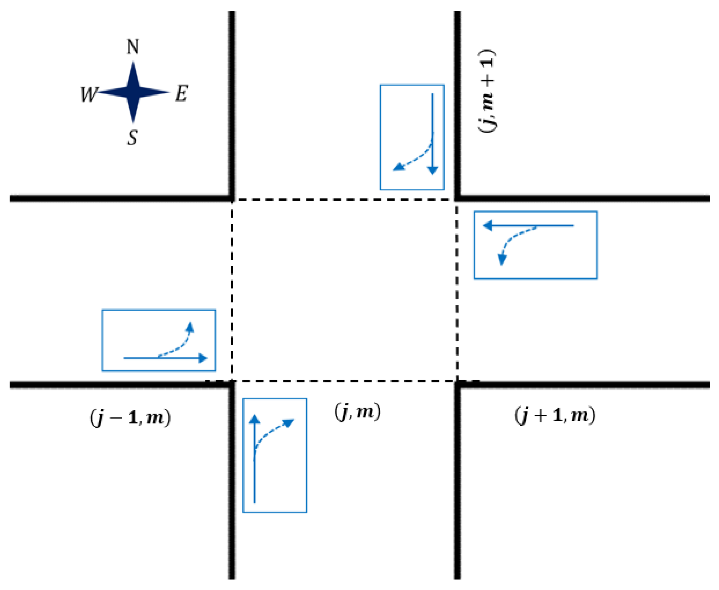
As shown in Figure 1, each intersection is regarded as a lattice, and some pedestrians continue to walk while others turn at the intersection. In Figure 1, the blue arrows indicate the pedestrian flow, and the dotted arrows indicate the pedestrian flow turning at the intersection.

There are four types of pedestrians to consider: eastbound, westbound, northbound, and southbound. They are assumed to move freely in all directions of positive $x$, negative $x$, positive $y$, and negative $y$. The density of eastbound, westbound, northbound, and southbound pedestrians at lattice point $\left(j,m\right)$ at time $t$ are denoted by ${\rho }_{x+}\left(j,m,t\right)$, ${\rho }_{x-}\left(j,m,t\right)$, ${\rho }_{y+}\left(j,m,t\right),$ and ${\rho }_{y-}\left(j,m,t\right)$, respectively. The flux of eastbound, westbound, northbound, and southbound pedestrians’ lattice position $\left(j,m\right)$ at time $t$ is expressed as $Q_{x+}\left(j,m,t\right), Q_{x-}\left(j,m,t\right), Q_{y+}\left(j,m,t\right),$ and $Q_{y-}\left(j,m,t\right),$ respectively. $Q\left(j,m,t\right)$ is the total flux at lattice position $\left(j,m\right)$ at time $t$. The continuous equation is:

$${\partial }_t{\rho }_{x+}(j,m,t)+c{c}_1{\rho }_0[Q_{x+}(j,m,t)-Q_{x+}(j-1,m,t)]=0$$

(1)

$${\partial }_t{\rho }_{x-}(j,m,t)+c(1-c_1){\rho }_0[Q_{x-}(j,m,t)-Q_{x-}(j+1,m,t)]=0$$

(2)

$${\partial }_t{\rho }_{y+}(j,m,t)+(1-c)c_2{\rho }_0[Q_{y+}(j,m,t)-Q_{y+}(j,m-1,t)]=0$$

(3)

$${\partial }_t{\rho }_{y-}(j,m,t)+(1-c)(1-c_2){\rho }_0[Q_{y-}(j,m,t)-Q_{y-}(j,m+1,t)]=0$$

(4)

where ${\partial }_t=\frac{\partial }{\partial t}, {\partial }_x=\frac{\partial }{\partial x}, and {\partial }_y=\partial /\partial y.$ Assuming the ratio of eastbound and westbound pedestrians to all pedestrians is $c$, southbound and northbound pedestrians possess $1-c$ percentage. The fraction of eastbound pedestrians in eastbound and westbound pedestrians is $c_1$, and the proportion of northbound pedestrians in northbound and southbound pedestrians corresponds to $c_2$ percentage. Other parameters are given in

Table 1. Symbols and their meanings in the four-way pedestrian traffic model.

Parameters and Symbols	Explanations
$+$	Positive direction
$-$	Negative direction
$a$	Pedestrian sensitivity coefficient (the inverse of the delay time $\tau$)
${\rho }_0$	Average density
${\rho }_c$	Critical safety density
$V\left(·\right)$	Optimal velocity function
$\left(j,m\right)$	Lattice position
${\rho }_{\left(j,m\right)}$	Local density at lattice $\left(j,m\right)$ at time $t$
$Q_{\left(j,m\right)}$	Traffic flow rate at lattice $\left(j,m\right)$ at time $t$
$v_{\left(j,m\right)}$	Average speed at lattice site $\left(j,m\right)$ at time $t$
${\beta }_1$,${\beta }_2$	Weights for eastbound and westbound pedestrians, respectively
${\gamma }_1$$,{\gamma }_2$	Weights for northbound and southbound pedestrians, respectively

.

According to the idea of the lattice hydrodynamic model [24], pedestrian flow in all directions is regulated by the total optimized flow. In four-way pedestrian traffic, when pedestrians change direction midway, it causes changes in pedestrian flow in the other direction, as shown in Figure 1. Therefore, the evolution equation of pedestrian flow in the positive $x$ direction can be obtained, where ${\beta }_1$ represents the weight of eastbound pedestrians on the road, and $1-{\beta }_1$ represents the weight of some northbound pedestrians turning eastbound.

$$\begin{array}{l}{\partial }_t{}^2{\rho }_{x+}(j,m)+a{\partial }_t{\rho }_{x+}(j,m)\\ +a{\rho }_0{}^{2}c{c}_1 \left\{{\beta }_{1}c{c}_1\left[V\left({\rho }_{j+1,m}\right)-V\left({\rho }_{j,m}\right)\right]+(1-{\beta }_1)(1-c)c_2\left[V\left({\rho }_{j,m+1}\right)-V\left({\rho }_{j-1,m+1}\right)\right]\right\}=0\end{array}$$

(5)

Then, in four-way pedestrian traffic, the evolution equation along the other direction of the road is as follows:

$$\begin{array}{l}{\partial }_t{}^2{\rho }_{x-}(j,m)+a{\partial }_t{\rho }_{x-}(j,m)\\ +a{\rho }_0{}^{2}c\left(1-c_1\right)\left[{\beta }_{2}c\left(1-c_1\right)\left[V({\rho }_{j-1,m})-V({\rho }_{j,m})\right]+(1-{\beta }_2)\left(1-c\right)\left(1-c_2\right)\left[V\left({\rho }_{j,m-1}\right)-V\left({\rho }_{j+1,m-1}\right)\right]\right]=0\end{array}$$

(6)

$$\begin{array}{l}{\partial }_t{}^2{\rho }_{y+}+a{\partial }_t{\rho }_{y+}\\ +a{c}_2(1-c){\rho }_0{}^2\left[{\gamma }_1(1-c)c_2\left[V({\rho }_{j,m+1})-V({\rho }_{j,m})\right]+(1-{\gamma }_1)c{c}_1\left[V\left({\rho }_{j+1,m}\right)-V\left({\rho }_{j+1,m-1}\right)\right]\right]=0\end{array}$$

(7)

$$\begin{array}{l}{\partial }_t{}^2{\rho }_{y-}(j,m)+a{\partial }_t{\rho }_{y-}(j,m)\\ +a{\rho }_0{}^2 \left(1-c\right)\left(1-c_2\right)\left\{{\gamma }_2\left(1-c\right)\left(1-c_2\right)\left[V({\rho }_{j,m-1})-V({\rho }_{j,m})\right]+(1-{\gamma }_2)c\left(1-c_1\right)\left[V\left({\rho }_{j-1,m}\right)-V\left({\rho }_{j-1,m+1}\right)\right]\right\}=0\end{array}$$

(8)

In order to simplify the calculation, assume that ${\gamma }_1={\gamma }_2=\gamma$ and ${\beta }_1={\beta }_2=\beta$. Then, pedestrians in the east–west direction (horizontal passage) have the same weight $\beta$ to move, and in this direction, the weight of turning pedestrians is expressed by $\left(1-\beta \right)$. Pedestrians move with the same weight $\gamma$ in the north–south direction (vertical passage), and the weight of turning pedestrians in this direction is expressed by $\left(1-\gamma \right)$.

Under periodic conditions, the total density at the lattice position $\left(j,m\right)$ at time $t \mathrm{is} \rho \left(j,m,t\right)={\rho }_{x+}\left(j,m,t\right)+{\rho }_{x-}\left(j,m,t\right)+{\rho }_{y+}\left(j,m,t\right)+{\rho }_{y-}\left(j,m,t\right)$. As a result, the following lattice density equation of four-way pedestrian flow is obtained.

$$\begin{array}{l}{\partial }_t{}^2\rho (j,m)+a{\partial }_t\rho (j,m)\\ +a\beta c^2\left\{c_1{}^2\left[V\left({\rho }_{j+1,m}\right)-V\left({\rho }_{j,m}\right)\right]+{\left(1-c_1\right)}^2\left[V({\rho }_{j-1,m})-V({\rho }_{j,m})\right]\right\}{\rho }_0{}^2\\ +a\gamma {\left(1-c\right)}^2\left\{c_2{}^2\left[V({\rho }_{j,m+1})-V({\rho }_{j,m})\right]+{\left(1-c_2\right)}^2\left[V({\rho }_{j,m-1})-V({\rho }_{j,m})\right]\right\}{\rho }_0{}^2\\ +a(1-\beta )c(1-c)\left\{c_1{c}_2\left[V\left({\rho }_{j,m+1}\right)-V\left({\rho }_{j-1,m+1}\right)\right]+\left(1-c_1\right)\left(1-c_2\right)\left[V\left({\rho }_{j,m-1}\right)-V\left({\rho }_{j+1,m-1}\right)\right]\right\}{\rho }_0{}^2\\ +a(1-\gamma )c\left(1-c\right)\left\{c_1{c}_2\left[V\left({\rho }_{j+1,m}\right)-V\left({\rho }_{j+1,m-1}\right)\right]+\left(1-c_1\right)\left(1-c_2\right)\left[V\left({\rho }_{j-1,m}\right)-V\left({\rho }_{j-1,m+1}\right)\right]\right\}{\rho }_0{}^2=0\end{array}$$

(9)

The velocity $V\left({\rho }_{j,m}\right)$ is called the optimal velocity function of the density ρ, which is defined as follows [25]:

$$V\left({\rho }_{j,m}\right)=\frac{v_{\max }}{2}\left[\tanh (\frac{2}{{\rho }_0}-\frac{{\rho }_{j,m}}{{\rho }_0{}^2}-\frac{1}{{\rho }_c})+\tanh (\frac{1}{{\rho }_c})\right]$$

(10)

3. Stability Analysis

The stability analysis of traffic flow focuses on the evolution of small disturbances in the traffic system over time and observes the change in the disturbance amplitude over time. Assuming that the uniform pedestrian flow has a constant density ${\rho }_0$ and velocity $V\left({\rho }_0\right)$ along with all directions, the steady-state solution of the pedestrian flow density Equation (9) can thus be obtained by Equation (11):

$${[{\rho }_{j,m},Q_{j,m}]}^T={[{\rho }_0,q_0]}^T$$

(11)

Suppose $y_{j, m}\left(t\right)$ is a small perturbation from the steady state: ${\rho }_{j,m}\left(t\right)={\rho }_0+y_{j, m}\left(t\right)$. Then, the linearized equation is obtained from Equation (9).

$$\begin{array}{l}{\partial }_t{}^2{y}_{j,m}+a{\partial }_t{y}_{j,m}\\ +a\beta c^2\left[c_1{}^2\left(y_{j+1,m}-y_{j,m}\right)+{\left(1-c_1\right)}^2\left(y_{j-1,m}-y_{j,m}\right)\right]{\rho }_0{}^2{V}^{\prime }\\ +a\gamma {\left(1-c\right)}^2\left[c_2{}^2\left(y_{j,m+1}-y_{j,m}\right)+{\left(1-c_2\right)}^2\left(y_{j,m-1}-y_{j,m}\right)\right]{\rho }_0{}^2{V}^{\prime }\\ +a(1-\beta )c(1-c)\left[c_1{c}_2\left(y_{j,m+1}-y_{j-1,m+1}\right)+\left(1-c_1\right)\left(1-c_2\right)\left(y_{j,m-1}-y_{j+1,m-1}\right)\right]{\rho }_0{}^2{V}^{\prime }\\ +a(1-\gamma )c\left(1-c\right)\left[c_1{c}_2\left(y_{j+1,m}-y_{j+1,m-1}\right)+\left(1-c_1\right)\left(1-c_2\right)\left(y_{j-1,m}-y_{j-1,m+1}\right)\right]{\rho }_0{}^2{V}^{\prime }=0\end{array}$$

(12)

where $V^{\prime }=\frac{\partial V\left(\rho \right)}{\partial \rho }{|}_{\rho ={\rho }_c}$. Expanding $y_{j, m}\left(t\right)$ in the Fourier modes, $y_{j, m}\left(t\right)=exp\left[ik\left(j+m\right)+zt\right]$. Substituting this into Equation (12), the following equation is yielded:

$$\begin{array}{l}{z}^2+az\\ +a\beta c^2\left[c_1{}^2\left(e^{ik}-1\right)+{\left(1-c_1\right)}^2\left(e^{-ik}-1\right)\right]{\rho }_0{}^2{V}^{\prime }\\ +a\gamma {\left(1-c\right)}^2\left[c_2{}^2\left(e^{ik}-1\right)+{\left(1-c_2\right)}^2\left(e^{-ik}-1\right)\right]{\rho }_0{}^2{V}^{\prime }\\ +a(2-\beta -\gamma )c(1-c)\left[c_1{c}_2\left(e^{ik}-1\right)+\left(1-c_1\right)\left(1-c_2\right)\left(e^{-ik}-1\right)\right]{\rho }_0{}^2{V}^{\prime }=0\end{array}$$

(13)

By expanding $z=z_1\left(ik\right)+z_2{\left(ik\right)}^2+\dots$ and inserting it into Equation (13) leads to the first- and second-order terms of coefficients in the expression of z, respectively:

$$z_1=-\left\{\beta c^2\left(2c_1-1\right)+\gamma {\left(1-c\right)}^2\left(2c_2-1\right)+(2-\beta -\gamma )c(1-c)\left[c_1+c_2-1\right]\right\}{\rho }_0{}^2{V}^{\prime }$$

(14)

$$z_2=-\frac{z_1{}^2}{a}-\frac{1}{2}\left\{\beta c^2\left(2c_1-1\right)+\gamma {\left(1-c\right)}^2\left(2c_2-1\right)+(2-\beta -\gamma )c(1-c)\left[1-c_1-c_2+2c_1{c}_2\right]\right\}{\rho }_0{}^2{V}^{\prime }$$

(15)

If $z_2$ is negative, the uniform steady-state flow becomes unstable for long-wavelength modes. When $z_2$ is positive, the uniform flow is stable. The neutral stability condition is obtained as:

$$-\frac{2{\left\{\beta c^2\left(2c_1-1\right)+\gamma {\left(1-c\right)}^2\left(2c_2-1\right)+(2-\beta -\gamma )c(1-c)\left(c_1+c_2-1\right)\right\}}^2{\rho }_0{}^2{V}^{\prime }}{\beta c^2\left(1-2c_1+2c_1{}^2\right)+\gamma {\left(1-c\right)}^2\left(1-2c_2+2c_2{}^2\right)+(2-\beta -\gamma )c(1-c)\left(1-c_2-c_1+2c_1{c}_2\right)}<a$$

(16)

When $\beta =\gamma =1.0$, Equation (16) satisfies the stability condition of Tian’s bidirectional pedestrian traffic model [27].

$$-\frac{2{\left\{c^2\left(2c_1-1\right)+{\left(1-c\right)}^2\left(2c_2-1\right)\right\}}^2{\rho }_0{}^2{V}^{\prime }}{c^2\left(1-2c_1+2c_1{}^2\right)+{\left(1-c\right)}^2\left(1-2c_2+2c_2{}^2\right)}<a$$

(17)

When $c_1=c_2=1.0, \beta \ne 1.0, \mathrm{and} \gamma \ne 1.0$, Equation (16) transforms into the stability condition for Tian’s lattice hydrodynamic model [26].

$$-2\left\{\beta c^2+\gamma {\left(1-c\right)}^2+(2-\beta -\gamma )c(1-c)\right\}{\rho }_0{}^2{V}^{\prime }<a$$

(18)

4. Nonlinear Analyses

Under the limited disturbance of pedestrian flow, the nonlinear analysis of the density evolution in Equation (9) of the pedestrian traffic flow is carried out. Considering the long-wave mode on a coarse-grained scale, near the critical point (${\rho }_c,a_c$), a small parameter $\epsilon$ is introduced, which represents the deviation from the critical point $a_c$. We introduce slow scales for space variables $j, m$ and time variable $t$ and define slow variables $X$ and $T$:

$$X=\epsilon \left(j+m+bt\right), T={\epsilon }^{3}t$$

(19)

where $0<\epsilon \ll 1$, $b$ is the undetermined constant, and the density is defined as:

$$\rho \left(j,m,t\right)={\rho }_c+\epsilon R\left(X,T\right)$$

(20)

Substituting Equations (19) and (20) into Equation (9), the nonlinear partial differential equation is obtained using Taylor expansion to the fifth order of small parameter $\epsilon$.

$$\begin{array}{l}{\epsilon }^2\left[b+\left[\beta c^2\left(2c_1-1\right)+\gamma {\left(1-c\right)}^2\left(2c_2-1\right)+(2-\beta -\gamma )c(1-c)\left(c_1+c_2-1\right)\right]{\rho }_0{}^2{V}^{\prime }\right]{\partial }_{x}R\\ +{\epsilon }^3\left\{\frac{b^2}{a}+\frac{1}{2}\left[\beta c^2\left(1-2c_1+2c_1{}^2\right)+\gamma {\left(1-c\right)}^2\left(1-2c_2+2c_2{}^2\right)+(2+\beta +\gamma )c(1-c)\left(c_1+c_2-1\right)\right]{\rho }_0{}^2{V}^{\prime }\right\}{\partial }_X{}^{2}R\\ +{\epsilon }^4\frac{1}{6}\left[\beta c^2\left(2c_1-1\right)+\gamma {\left(1-c\right)}^2\left(2c_2-1\right)+(2-\beta -\gamma )c(1-c)\left(c_1+c_2-1\right)\right]{\rho }_0{}^2{V}^{\prime }{\partial }_X^{3}R\\ +{\epsilon }^4\frac{1}{6}\left[\beta c^2\left(2c_1-1\right)+\gamma {\left(1-c\right)}^2\left(2c_2-1\right)+(2-\beta -\gamma )c(1-c)\left(c_1+c_2-1\right)\right]{\rho }_0{}^2{V}^{‴}{\partial }_X{R}^3\\ +\frac{1}{24}{\epsilon }^5\left[\beta c^2\left(1-2c_1+2c_1{}^2\right)+\gamma {\left(1-c\right)}^2\left(1-2c_2+2c_2{}^2\right)+(2+\beta +\gamma )c(1-c)\left(c_1+c_2-1\right)\right]{\rho }_0{}^2{V}^{\prime }{\partial }_X^{4}R\\ +\frac{1}{12}{\epsilon }^5\left[\beta c^2\left(1-2c_1+2c_1{}^2\right)+\gamma {\left(1-c\right)}^2\left(1-2c_2+2c_2{}^2\right)+(2+\beta +\gamma )c(1-c)\left(c_1+c_2-1\right)\right]{\rho }_0{}^2{V}^{‴}{\partial }_X^2{R}^3\\ +{\epsilon }^4{\partial }_{T}R+2{\epsilon }^5\frac{b}{a}{\partial }_X{\partial }_{T}R=0\end{array}$$

(21)

where $V^{\prime }\left({\rho }_c\right)=\frac{\partial V\left(\rho \right)}{\partial \rho }{|}_{\rho ={\rho }_c}$, $V^{‴}\left({\rho }_c\right)=\frac{{\partial }^{3}V\left(\rho \right)}{\partial {\rho }^3}{|}_{\rho ={\rho }_c}$. The second- and third-order terms of ε are eliminated from Equation (21) by taking $b=-\left[\beta c^2\left(2c_1-1\right)+\gamma {\left(1-c\right)}^2\left(2c_2-1\right)+\left(2-\beta -\gamma \right)c\left(1-c\right)\left(c_1+c_2-1\right)\right]{\rho }_0{}^2$. By eliminating the second-order and third-order terms of $\epsilon$ in Equation (21), the simplified equation is obtained near the critical point $\left(a_c,{\rho }_c\right)$.

$$a=a_{\mathrm{c}}\left(1-{\epsilon }^2\right)$$

(22)

Equation (21) transforms into Equation (23):

$${\epsilon }^4\left[{\partial }_{T}R-g_1{\partial }_X^{3}R+g_2{\partial }_{X}R{ }^3\right]+{\epsilon }^5\left[g_3{\partial }_X^{2}R+g_4{\partial }_X^{4}R+g_5{\partial }_X^2{R}^3\right]=0$$

(23)

We carry out the following transformation:

$$T^{\prime }=g_{1}T,R=\sqrt{\frac{g_1}{g_2}}{R}^{\prime }$$

(24)

Thus, the mKdV equation with $O\left(\epsilon \right)$ is obtained:

$${\partial }_{ \mathrm{T}\prime }{R}^{\prime }-{\partial }_X^3{R}^{\prime }+{\partial }_X{R^{\prime }}^3+\epsilon M[R^{\prime }]=0$$

(25)

where $\mathrm{M}\left[R^{\prime }\right]=\sqrt{\frac{1}{g_1}}\left[g_3{\partial }_X^2{R}^{\prime }+\frac{g_1{g}_5}{g_2}{\partial }_X^2{R}^{\prime 3}+g_4{\partial }_X^4{R}^{\prime }\right]$; ignoring the $O\left(\epsilon \right)$ term, the solution of the kink–antikink wave in Equation (23) is given.

$${R^{\prime }}_0(X,T^{\prime })=\sqrt{c}\tanh \sqrt{\frac{c}{2}}(X-c{T}^{\prime })$$

(26)

where $R_0^{,}\left(X,T^{\prime }\right)$ should satisfy the solvable condition:

$$({R^{\prime }}_0,\mathrm{M}[R^{\prime }])=\underset{-\infty }{\overset{+\infty }{{\displaystyle \int }}}dX{R^{\prime }}_0(X,T^{\prime })M[(X,T^{\prime })]$$

(27)

By integration, the propagation velocity of the kink–antikink wave is obtained:

$$c=\frac{5g_2{g}_3}{2g_2{g}_4-3g_1{g}_5}$$

(28)

The solution to the mKdV Equation (23) is given as follows:

$$\rho (j,m,t)={\rho }_c+\epsilon \sqrt{\frac{g_{1}c}{g_2}}\tanh (\sqrt{\frac{c}{2}}(X-c{g}_{1}T))$$

(29)

The amplitude of the kink–antikink wave is:

$$A=\sqrt{\frac{g_{1}c}{g_2}(\frac{a_c}{a}-1)}$$

(30)

The values of each coefficient of $\mathrm{g}$ are expressed as follows:

$$g_1=-\frac{1}{6}\left[\beta c^2\left(2c_1-1\right)+\gamma {\left(1-c\right)}^2\left(2c_2-1\right)+(2-\beta -\gamma )c(1-c)\left(c_1+c_2-1\right)\right]{\rho }_0{}^2{V}^{\prime }$$

$$g_2=\frac{1}{6}\left[\beta c^2\left(2c_1-1\right)+\gamma {\left(1-c\right)}^2\left(2c_2-1\right)+(2-\beta -\gamma )c(1-c)\left(c_1+c_2-1\right)\right]{\rho }_0{}^2{V}^{‴}$$

$$g_3=\frac{1}{a_c}{\left\{\left[\beta c^2\left(2c_1-1\right)+\gamma {\left(1-c\right)}^2\left(2c_2-1\right)+(2-\beta -\gamma )c(1-c)\left(c_1+c_2-1\right)\right]{\rho }_0{}^2{V}^{\prime }\right\}}^2$$

$$\begin{array}{ll}{g}_4=& \frac{1}{24}\left[\beta c^2\left(1-2c_1+2c_1{}^2\right)+\gamma {\left(1-c\right)}^2\left(1-2c_2+2c_2{}^2\right)+(2+\beta +\gamma )c(1-c)\left(c_1+c_2-1\right)\right]{\rho }_0{}^2{V}^{\prime }\\ & -\frac{2b}{6a_{\mathrm{c}}}\left[\beta c^2\left(2c_1-1\right)+\gamma {\left(1-c\right)}^2\left(2c_2-1\right)+(2-\beta -\gamma )c(1-c)\left(c_1+c_2-1\right)\right]{\rho }_0{}^2{V}^{\prime }\end{array}$$

$$\begin{array}{ll}{g}_5=& -\frac{2b}{6a_{\mathrm{c}}}\left[\beta c^2\left(2c_1-1\right)+\gamma {\left(1-c\right)}^2\left(2c_2-1\right)+(2-\beta -\gamma )c(1-c)\left(c_1+c_2-1\right)\right]{\rho }_0{}^2{V}^{‴}\\ & +\frac{1}{12}\left[\beta c^2\left(1-2c_1+2c_1{}^2\right)+\gamma {\left(1-c\right)}^2\left(1-2c_2+2c_2{}^2\right)+(2+\beta +\gamma )c(1-c)\left(c_1+c_2-1\right)\right]{\rho }_0{}^2{V}^{‴}\end{array}$$

The solution to the kink–antikink wave represents the coexistence phase, and the coexistence curve can be expressed as follows:

$$A=\sqrt{\frac{g_{1}c}{g_2}(\frac{a_c}{a}-1)}$$

(31)

where ${\rho }_{j,m}={\rho }_c-A$ represents the free flow of a low-density pedestrian traffic flow, and ${\rho }_{j,m}={\rho }_c+A$ represents the congested phase of a high-density pedestrian traffic flow.

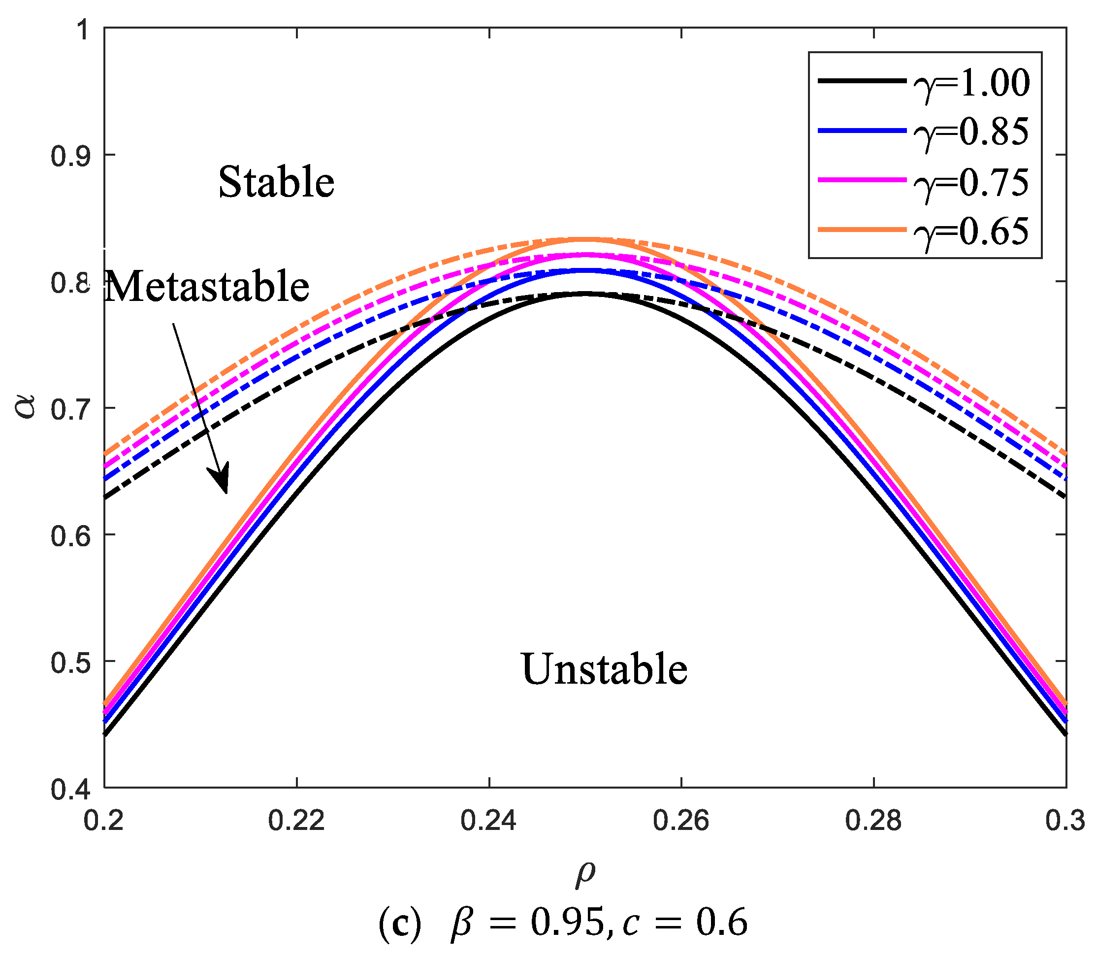
Figure 2b and Figure 2c is the $\left(\rho ,a\right)$ plane phase diagram of the traffic model under different $\gamma$ and $\beta$ values. The solid line and the dashed line represent the neutral stability curve and the coexistence curve, respectively. According to the pedestrian traffic flow stability theory, the phase diagram can be divided into three different regions: the stable region over the coexistence curve, the metastable region between the coexistence curve and the neutral stability curve, and the unstable region below the neutral stability curve.

Figure 2a shows the four-way pedestrian traffic phase diagram with fixed pedestrian turning weights. In a fixed $\gamma$ and $\beta$, when $c$ increases to 0.4, the critical point $a_c$ decreases gradually, and close to 0.8, the unstable area decreases significantly. This shows that the proportion of the pedestrian flow in the horizontal passage has a great influence on the stability of pedestrian traffic. When the proportion of the pedestrian flow in the horizontal passage increases, the distribution of the pedestrian flow in the four directions of the passage tends to be even, which enhances the stability of the pedestrian traffic system and helps to suppress pedestrian traffic congestion. The effect of pedestrian turning on four-way pedestrian traffic is shown in Figure 2b,c. In Figure 2b, the proportion of pedestrians turning into the horizontal passage will increase as $\beta$ decreases. It can be seen that the unstable area continues to increase, that is, the pedestrian flow turns at the road intersection, which is not conducive to traffic stability. When $\beta =1.0$, the pedestrian flow in the vertical passage is prohibited from turning, the critical point $a_c$ is significantly reduced, and the stable area is also increased. In Figure 2c, the distribution of the initial density is changed, and $c=0.6$ is taken. With the decrease in $\gamma$, the proportion of turning pedestrians in the vertical passage increases, and the unstable area increases continuously, which enables pedestrian congestion, and the stability of the pedestrian traffic system also decreases. This indicates that the turning of the pedestrian flow in four-way pedestrian traffic easily leads to traffic instability and traffic congestion. As the proportion of pedestrians turning increases, traffic congestion is more likely to be exacerbated.

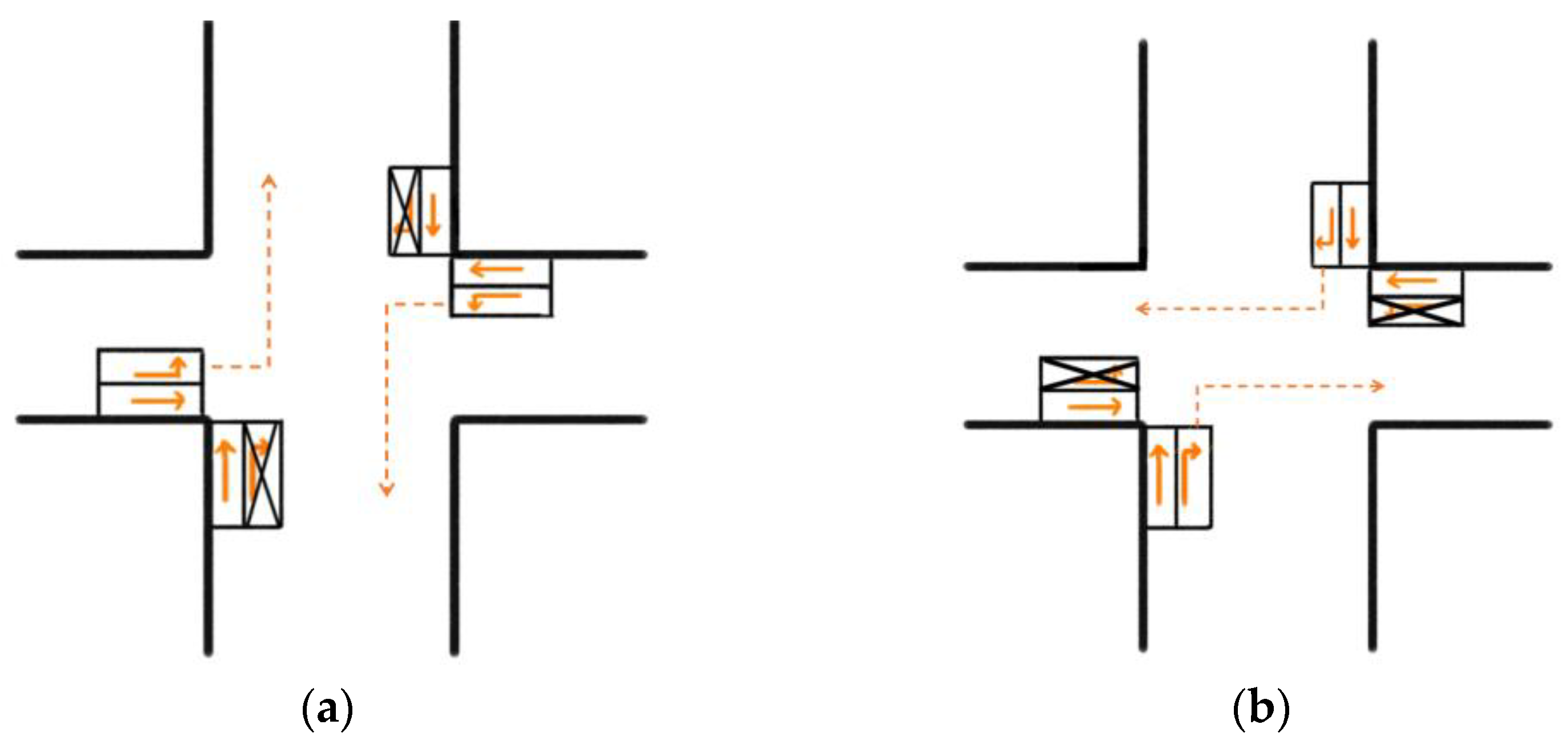
Therefore, electronic road signs can be set up at the intersection to guide pedestrians to turn to walk at different times. As shown in Figure 3, the orange arrows represent road electronic signs that guide the pedestrian flow, and the place marked ⊠ indicates that pedestrians are not allowed to turn at this intersection. As shown in Figure 3a, only pedestrians in the horizontal passage are allowed to turn in four-way pedestrian traffic. As shown in Figure 3b, only pedestrians in vertical passages are allowed to turn in four-way pedestrian traffic.

5. Numerical Simulations

The influence of the turning of pedestrian flow on the stability of the traffic system in four-way pedestrian traffic is further studied through numerical simulation. For the convenience of numerical simulation, Equation (9) is rewritten into the following difference form:

$$\begin{array}{l}{\rho }_{j,m}(t+2\tau )-2{\rho }_{j,m}(t+\tau )+{\rho }_{j,m}(t)+a\tau [{\rho }_{j,m}(t+\tau )-{\rho }_{j,m}(t)]\\ +a{\tau }^2\beta c^2\left[c_1{}^2\left[V\left({\rho }_{j+1,m}\right)-V\left({\rho }_{j,m}\right)\right]+{\left(1-c_1\right)}^2\left[V({\rho }_{j-1,m})-V({\rho }_{j,m})\right]\right]{\rho }_0{}^2\\ +a{\tau }^2\gamma {\left(1-c\right)}^2\left[c_2{}^2\left[V({\rho }_{j,m+1})-V({\rho }_{j,m})\right]+{\left(1-c_2\right)}^2\left[V({\rho }_{j,m-1})-V({\rho }_{j,m})\right]\right]{\rho }_0{}^2\\ +a{\tau }^2(1-\beta )c(1-c)\left[c_1{c}_2\left[V\left({\rho }_{j,m+1,}\right)-V\left({\rho }_{j-1,m+1,}\right)\right]+\left(1-c_1\right)\left(1-c_2\right) \left[V\left({\rho }_{j,m-1}\right)-V\left({\rho }_{j+1,m-1}\right)\right]\right]{\rho }_0{}^2\\ +a{\tau }^2(1-\gamma )c(1-c)\left[c_1{c}_2 \left[V\left({\rho }_{j+1,m}\right)-V\left({\rho }_{j+1,m-1}\right)\right]+\left(1-c_1\right)\left(1-c_2\right) \left[V\left({\rho }_{j-1,m}\right)-V\left({\rho }_{j-1,m+1}\right)\right]\right]{\rho }_0{}^2=0\end{array}$$

(32)

Assumed that the four-way pedestrian traffic consists of $N\times N$ lattices ($N=140$). The numerical simulation is carried out with periodic boundary conditions, and the initial density of the lattice point is set to:

$${\rho }_{j,m}(0)={\rho }_{j,m}(t)=\{\begin{array}{l}{\rho }_0-\delta \hspace{1em}\hspace{1em}j=m=N/2\\ {\rho }_0+\delta \hspace{1em}j=m=N/2+1 \\ {\rho }_0\hspace{1em}\hspace{1em}\hspace{1em}\hspace{1em}otherwise\end{array}$$

(33)

where the initial perturbation $\delta \left(\delta =0.1\right)$ is added to the lattice position $\left(j,m\right)$, and the other parameters are ${\rho }_0=0.2$, $v_{max}=2.0$,$\alpha =1$.2, and c₁ = c₂ = 0.105.

From the stability analysis, it is clear that pedestrian flow turning has an important effect on four-way pedestrian traffic. To visually analyze the role of pedestrian turning in four-way pedestrian traffic, we analyze the pedestrian density variation at all lattice locations. As shown in Figure 4, the black dots indicate that the pedestrian density at this lattice position is greater than the average pedestrian density ${\rho }_0$. Determine the proportion of east–west (horizontal passage) pedestrians to all pedestrians in the initial state as $c$ is 0.4, and fix the pedestrian turning weight $\gamma =0.95$ for southbound and northbound traffic (vertical passage).

In Figure 4a, it can be seen that taking $\beta =0.65$, when the time step is T = 1500, the pedestrians are distributed throughout the area, the local area presents a high density of pedestrians, and pedestrian congestion occurs. Comparing Figure 4a–c, we know that with the increase in $\beta$, the pedestrian congestion in the space is effectively suppressed. When $\beta$ increases to 0.85, the congestion in four-way pedestrian traffic almost disappears. This also means that the turning weight for southbound and northbound (vertical passages) pedestrians decreases as $\beta$ increases. The congestion area begins to dissipate from the south and north directions first, which corresponds to the shrinkage of the black area in the Y-direction in Figure 4. The above analysis shows that paying more attention to the uniform distribution of pedestrians along the road can effectively suppress the occurrence of pedestrian congestion. On the contrary, the turning effect of pedestrians will stimulate traffic congestion, which is not conducive to improving the stability of the traffic system. The obtained results are consistent with the stability analysis.

As shown in Figure 5, fix the $\mathrm{lattice} \mathrm{position} m=65$, and observe the density change at the $x$ lattice position at different times. With an increasing value of $\beta$, the density wave gradually tends to be stable, and the weight of the pedestrian turning in the vertical passage also decreases, which is consistent with the results obtained in Figure 2. In order to reduce the possibility of congestion and effectively control traffic, we try to set up electronic road signs in four-way pedestrian traffic. In Figure 5d, take $\beta$ as $1.0$, that is, the pedestrians in the vertical passage will no longer turn. By comparing and analyzing Figure 5a and Figure 5d, it can be seen that traffic congestion is under control.

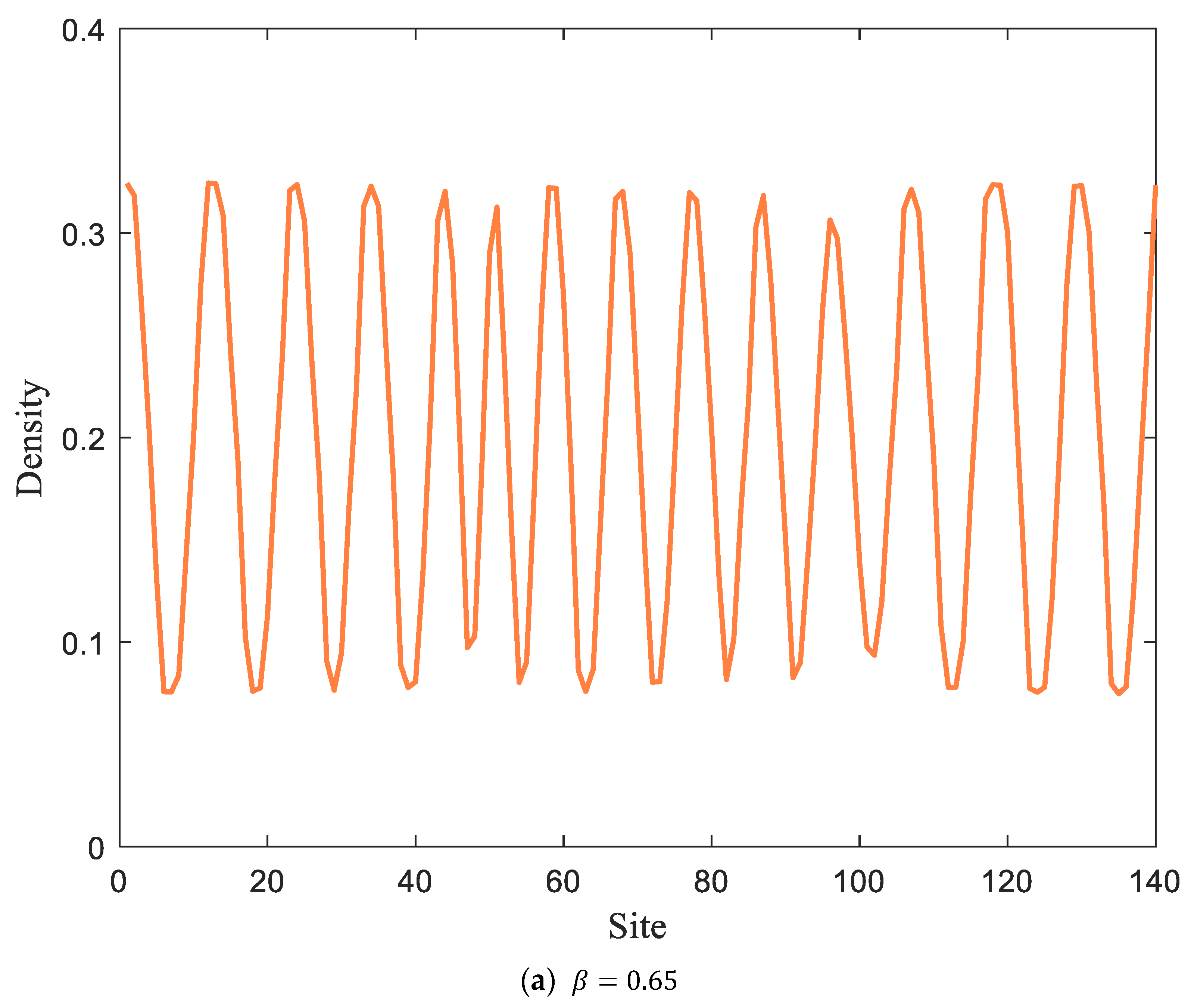
The density profile corresponding to Figure 5 at time $t=10,000$ is given in Figure 6. In the comparative analysis, it can be concluded that the increase in parameter $\beta$ causes the density wave to gradually stabilize, i.e., reducing the proportion of pedestrian turns in the vertical passage can effectively suppress traffic congestion. With the introduction of electronic road signs, as shown in Figure 6d, it can be seen that pedestrian traffic fluctuations have stabilized, and traffic congestion has been controlled.

6. Conclusions

It is of great practical value to study the influence of the turning of pedestrian flows at crossroads (intersections, underpasses, etc.) on the stability of the traffic system. Based on the pedestrian traffic flow, a four-way traffic lattice hydrodynamics model with turning capacity is proposed. The stability conditions are derived from the stability analysis and use nonlinear analysis methods to derive the mKdV equation describing the pedestrian congestion density wave. The solution to the kink–antikink density wave corresponding to the mKdV equation is obtained. The traffic phase diagram analysis shows that the unstable area increases with the increase in pedestrian turning weight. The results of numerical simulation are consistent with the theoretical analysis. Through numerical simulation, the density spatiotemporal pattern and traffic patterns of pedestrian flow evolution under different traffic conditions are studied in detail. An important conclusion to be drawn through the detailed research in this paper is that for the actual pedestrian traffic in all directions, the balanced distribution of pedestrian flow in horizontal and vertical channels is conducive to the stability of pedestrian traffic, whereas pedestrian turns cause traffic congestion for pedestrians, which is not conducive to the smooth flow of pedestrian traffic and may even cause crowd stampede accidents. Moreover, the establishment of electronic road signs can suppress congestion in four-way pedestrian traffic.