Abstract
Synthetic time series created from historical streamflow data are thought of as substitute events with a similar likelihood of recurrence to the real event. This technique has the potential to greatly reduce the uncertainty surrounding measured streamflow. The goal of this study is to create a synthetic streamflow model using a combination of Markov chain and Fourier transform techniques based on long-term historical data for the Nile River. First, the Markov chain’s auto-regression is applied, in which the data’s trend and seasonality are discovered and eliminated before applying the Pearson III distribution function. The Pearson III distribution function is substituted by a discrete Fourier transform (DFT) technique in the second approach. The applicability of the two techniques to simulate the streamflow between 1900 and 1999 is evaluated. The ability of the generated series to maintain the four most important statistical properties of the samples of monthly flows, i.e., the mean, standard deviation, autocorrelation lag coefficient, and cumulative distribution, was used to assess the quality of the series. The results reveal that the two techniques, with small differences in accuracy, reflect the monthly variation in streamflow well in terms of the three mentioned parameters. According to the coefficient of determination (R2) and normalized root mean square error (NRMSE) statistics, the discrete Fourier transform (DFT) approach is somewhat superior for simulating the monthly predicted discharge.
1. Introduction
Synthetic series derived from a sample of observed streamflow are regarded as alternate events with an admittedly equal probability of occurrence as the observed event. Synthetic data analysis holds its significance due to its applications in many fields, including reservoir planning, the control of floods and droughts, irrigation projects, and hydroelectric dam operation [1]. This technique has the potential to greatly reduce the level of uncertainty surrounding measured streamflow [2]. It also helps with the management of the currently available water resources by providing a better understanding of the past, present, and upcoming changes in streamflow by studying historical data [3]. It can even be used to build multivariate models that take both spatial and temporal variations in river streamflow into account [4]. By simulating the streamflow of the river, the beneficiary nations that rely on the Nile for freshwater can also find solutions to a variety of economic, geological, and even hydro-political issues.
A common technique to study river streamflow is to use a rainfall-runoff model along with a synthetic weather generator [5,6]. Nassar et al. [7] evaluated the performance of the Extended Streamflow Prediction (ESP) and the European Center for Medium-Range Weather Forecasting (ECMWF S4) models. The flow was forecast up to three months in advance in monthly time steps for each year from 2005 to 2011 in the Blue Nile Basin, and the results showed good connections between the two methods and the actual flow. However, the model required a huge amount of highly uncertain hydrological and metrological data, which affected the model’s accuracy. These uncertainties can be removed by direct synthetic streamflow methods [8].
Many researchers have been interested in creating statistical simulations for hydrological systems with autoregressive analysis methods. The most prominent of these is the “Auto Regressive Integrated Moving Average” (ARIMA) modeling technique, which has an abundance of studies in the literature [9,10,11,12]. Elganiny and Eldwer [13] used the SARIMA model and deseasonalized ARMA (DARMA) models to simulate monthly streamflow in the Nile River and its tributaries, as well as to forecast and compare the streamflow one month ahead. The findings show that for monthly streamflow in rivers, DARMA models outperform SARIMA models. Mohamed [14] used a well-known linear stochastic SARIMA model to forecast the monthly flow of the White Nile River in Malakal station, located in South Sudan, for the period 1970–2013. The model was found to be adequate for forecasting three successive years of monthly flow at Malakal station. Sharma et al. [15] claim that because these models’ autocorrelation dramatically declines as lag time grows, they can only be used to reproduce a short-range dependence. As a result, neither the pattern of linkage between flows in different months nor the seeming stability of yearly flows is guaranteed by them [16]. Consequently, they should not be employed in situations where long-term dependability is crucial [17].
A Markov model with time-varying parameters is another statistical method used by Salas [18], Pathak [19], and Al-Alati et al. [20]. Using this method, Pathak [19] examined 78 stream gauges in Maryland and produced a synthetic continuous daily hydrograph for rivers with gauged data. Prairie et al. [21] proposed that they may be used in conjunction with nonparametric techniques, such as k-nearest neighbors, while Pender et al. [5] stated that these models took into account the likelihood that certain hydrological conditions would change.
Additionally, Mehrotra et al. [22] proposed a stochastic simulation method for rainfall amount at different rainfall gauge stations using a method combining the “Nonhomogeneous Hidden Markov Model” (NNHMM) and a “Kernel Density Estimation” (KDE) method as a means of assessing the impact of climate change on rainfall amount in a particular region.
While streamflow patterns are usually non-linear and non-stationary, traditional statistical models, such as ARIMA models, are linear and do not sufficiently represent the non-linearity of streamflow [22]. Models based on machine learning techniques, such as ANN and GA, are another feasible alternative for time series modeling [23,24,25]. However, these processes are described as “black box” methods because interpreting the underlying algorithms can be challenging [26].
Another approach is to apply the Fourier transform (FT) analysis. The idea behind this method is to analyze the time series by converting it from the time domain to the frequency domain [27]. Chong et al. [28] investigated the behavior of the wavelet transform (WT) and the FT in a simulation of streamflow over the Johor River. They found that the WT is more suitable than the FT because it exhibits good extraction of the time and frequency characteristics, especially for a nonstationary data series. Because of the assumption that the analyzed data is periodic at T-equidistant time observations, this method is not very useful in its basic form when the intended result is time series forecasting [26]. Alternatively, it is possible to use this method in conjunction with statistical techniques [29,30,31,32].
Anderson et al. [33] developed synthetic flows by combining Fourier–ARMA modeling with an accurate representation of the model residuals and applied it to a series depicting average weekly flows on the Fraser River near Hope, B.C., Canada. Brunner et al. [29] used a combination of phase randomization simulation and a flexible four-parameter kappa distribution to apply and evaluate his method on a set of four Swiss catchments. The findings revealed that the phase randomization-based stochastic streamflow generator produced a realistic streamflow time series in terms of distributional features and temporal correlation. Cross-correlation among sites, on the other hand, was shown to be underestimated in several circumstances.
This work seeks to integrate the Markov chain approach with the Fourier transform technique to optimize the advantages of the two models. The Markov chain model using the Pearson III distribution function was first used. The Pearson III distribution function was then replaced with a Fourier transformation [18]. The monthly water discharge for the Nile River at Aswan is used as our study area for this research. This study presents a modular and expandable technique that is also a simple data-based analysis process. This technique may be used to construct synthetic streamflow as an alternative event with the same probability of occurrence as the measured one.
2. River Nile
Egypt is a water-stressed country with an estimated annual water share per capita of 337 m3 by 2025 [34], which confirms that it lies below the water poverty line of 1000 m3/capita [35] by approximately 66.3%. It depends mainly on the River Nile for 95% of its water requirements. In 2016, the country’s annual estimated water deficit was 13.5 billion cubic meters, and this is expected to reach 26 billion by 2025 [36]. Another looming problem that threatens the country is climate change. The increase in the average global temperature is jeopardizing not only the water supply but also the population’s food security, as well as the economic sector in general [37,38], not to mention other negative effects, such as the transmissibility of diseases [39] and social problems [40]. However, projects by decision-makers in Egypt are underway to combat this threat [41,42].
Therefore, understanding the hydrological processes that govern the River Nile’s water discharge is imperative for formulating any plans that deal with water shortage in Egypt. Meanwhile, the Nile River Basin is characterized by complex hydrology due to the uneven distribution of water resources among its sub-basins, coupled with climate change and the variation in its topographical composition, beginning with the mountainous areas of the upper Kagera, White Nile, Blue Nile, and Tekeze–Atbara rivers, and extending from the lower reaches to the Nile delta. Some subbasins, such as the Tekezé, become dry at periods during the year, while others, such as the Blue Nile, never become dry owing to the consecutive rainfall seasons. Both types of sub-basins have an impact on the water flowing at Aswan. This is the case for the examined data in this study since they are regarded as feeders to this reach of the river [43].
The Nile River is the longest in the world, with a total length of 6825 km, and it covers a drainage area of about 3.2 million km2 [44]. It supplies water to more than 238 million people [44]. The river has three main sources, which are the Ethiopian Plateau, the Equatorial Lakes Plateau, and the Bahr El Ghazal Basin. The Ethiopian Plateau contributes almost 86% of the natural flow at Aswan. The Equatorial Plateau is the source of the White Nile, which contributes to almost 14% of the natural flow at Aswan. Finally, the Bahr El Ghazal Basin contributes almost no flow to the natural flow at Aswan [44].
While the northern regions of the Nile (Egypt and Sudan) have almost rainless winters, the southern regions in Ethiopia experience heavy rains in winter (more than 1520 mm) [45]. In summer, most of the northern region becomes arid as the northeast trade winds take effect between October and May. Besides being a source of fresh water, common activities along the river include agriculture, fishing, recreation, transportation, and energy generation via hydroelectric dams.
The Nile River was chosen as a study area because of its great importance, the availability of long flow records, contemporary as well as older, and the additional historical information on its behavior, which give the Nile the advantage of being an ideal test case for identifying and understanding hydrological behaviors, and for model development [46].
3. Methodology
A dataset for the monthly discharge of the Nile River’s estimated streamflow arriving at Aswan was used [47,48]. The time series had 1195 recorded observations from January 1900 to July 1999, as shown in Figure 1a. The minimum monthly average discharge is 2.23 BCM/month in June, while the maximum monthly average discharge is 20.35 BCM/month in September, as shown in Figure 1b.
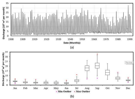
Figure 1.
(a) Time series for the Nile River monthly discharge records (from January 1900 to July 1999); (b) Nile River monthly discharge box and whisker plot.
3.1. Process Description
This process is structured into two main phases, a time series decomposition phase that’s based on Markov Chains [18,19,20], and a stochastic analysis phase. Our focus here is synthetic data generation. As in the generation of time series datasets that can represent the observed time series (original dataset) in a statistical sense. We also examine the effects of using two different stochastic analysis approaches. The first is the Pearson III distribution, and the second is the Fourier transformation. Figure 2 shows the flowchart describing the main steps in this model. The model is created in an Excel spreadsheet using VBA macros.
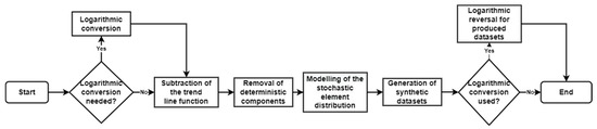
Figure 2.
Analysis process flowchart.
3.2. Data Decomposition
The input is the observed time series data. Whether in their original form or the logarithmic one, a Mann–Kendall (MK) non-parametric test is used to investigate the direction of a variable’s trend. This is a simple method to determine whether the general trend of a time series is increasing, decreasing, or remaining stable within a certain range [49,50]. This test is to determine how strongly correlated the dependent variable (monthly discharge) is with the independent variable (time in months). A positive value for the Z score statistic (Zs) indicates an upward trend, while a negative value indicates the opposite (a value approaching zero indicates a weak trend). This step is important to determine how influential the trend component is on the model. The interested reader is referred to D. R. Helsel and R. M. Hirsch [51] for the methodology behind the Mann–Kendall process. Equation (1) represents a linear trend for our time series, as follows:
where is the dependent variable’s value after removing the trend component; is the dependent variable’s value before removing the trend component; is the trend component given from regression analysis. Using the mean and standard deviation, seasonal effects are identified and removed, as follows:
where is the value that is free of seasonality; is the original value at time t; is the seasonal average value for y; is the seasonal standard deviation for y. The data is de-correlated using a lag-one correlation. The de-correlated K values can be computed as in the following Equation (3):
where is the de-correlated value at the ith observation and the jth season; is the correlated value at the ith observation; is the lag-one correlation coefficient for the jth season.
3.3. Stochastic Analysis
The de-correlated values for each season are arranged ascendingly and ranked, then the percentile of each ranked value is calculated using the Weibull formula, as follows:
where is the probability of observation at rank i, i is the observation’s rank; n is the total number of observations. The next two sections discuss each of the employed variations that were used for stochastic analysis and simulation.
3.4. Pearson III Distribution Method
Pearson III and lognormal distribution models were the best-fit functions for maximum streamflow [50]. Based on these results, the normal noise could be best predicted using the Pearson III distribution. The three parameters, namely the shape, scale, and shift, can be calculated using the following Equations (5)–(7):
where is the shape at the jth season; is the coefficient of skew at the jth season; is the scale at the jth season; is the shift at the jth season. The inverse Pearson III density function can be described with Equation (8), as follows:
where x is a random value between 0 and 1.
3.5. Discrete Fourier Transform Method
The DFT is used to simulate the time series for the study area. The logarithmic conversion was still used in the analytical process by following the previous model and replacing the Pearson III distribution with DFT. Converting the time series , where , to the frequency domain can be achieved using the DFT Equation (9) and its inverse (10) [52], as follows:
where is a dataset in the time domain; is a dataset in the frequency domain; , and (imaginary number); k is a discrete number variable; N is the total number of time series points. Knowing that , we can conclude that . Let . Using Euler’s formula, this can be further simplified as follows [53]:
Let and . The amplitude φ and initial phase α for each harmonic wave of frequency k can be calculated using the following Equations (12) and (13):
In a standard Fourier transformation, one only needs to calculate the amplitude and initial phase parameters per harmonic frequency, then re-construct the time series by computing the cosine waves for each frequency and combining them using Equation (10). However, the intention here is to simulate the stochastic, stationary dataset through phase randomization within a range of 0 to 2π for each harmonic wave while leaving the amplitude parameter intact. Random number generation algorithms used by modern software can be used to achieve this.
Note that for each of the two stochastic analysis approaches, a total of 100 random iterations were generated. This was carried out to test the simulations’ skill at capturing the random element in the observed dataset.
3.6. Data Reconstruction
The seasonality-free data (or Z values) with zero mean and unit variance are calculated by adding the autocorrelation component using the following equation:
where is the seasonality-free value at the ith observation; is the lag-one autocorrelation coefficient at the ith observation and the jth season; is the random value at the ith observation. However, it is worth noting that at i = 1, is replaced by a random value between zero and one. The seasonal mean and standard deviation are then added to each Z value as follows:
where is the detrended value at the ith observation and the jth season; is the mean at the jth season; is the standard deviation in the jth season.
Depending on the trend function used in the regression analysis, the simulated values for the hydrological parameter are calculated. In the case of a linear trend with only slope and intercept parameters, the following equation is used to add the trend function:
where is the synthetic value for the dependent variable with an added trend at the ith observation; is the trend line’s intercept parameter; is the trend line’s slope parameter; is the value for the independent variable (time) at the ith observation.
To evaluate the synthetic model, the mean, standard deviation, and temporal autocorrelation structure of the observed sequence are often expected to be reproduced by a synthetic streamflow generation process. Borgomeo et al. [1] suggested that some parameters be included in the evaluation of the synthetic model, including monthly mean, median standard deviation, skew coefficient, quantiles, monthly autocorrelation in addition to annual standard deviation, and autocorrelation.
The NRMSE statistic was calculated and normalized as shown in Equation (17) [54]. Note that σ is the standard deviation statistic for the observed dataset. Equation (17) is as follows:
The KGE (Kling–Gupta efficiency) and NSE (Nash–Sutcliffe efficiency) coefficients were also computed to measure the accuracy of the synthetic data [55,56] using the following Equations (18) and (19), respectively:
where r is the Pearson coefficient, is the standard deviation for the synthetic time series, is the standard deviation for the original time series, is the average for the synthetic time series, and is the average for the original time series. Equation (19) is as follows:
where is the value for the original time series at the ith observation, is the value for the synthetic time series at the ith observation, and is the average value for the original time series.
4. Results
Before applying the model, the measured monthly discharge values were converted to base 10 logarithm values to circumvent the generation of negative values in the synthetic datasets.
The Mann–Kendall test was conducted to measure the influence of the trend component on the time series. For this dataset, Zs = 5.54 and τ = 0.107, which indicates a slight upwards general trend in the data. The linear trend equation between the annual yearly date (X) starting from the first year (X0) and the log of the monthly discharge ( is estimated using Equation (18) and subtracted from the original data.
The linear trend equation between the annual yearly date (X) starting from the first year (X0) and the log of the monthly discharge ( is estimated using the following Equation and subtracted from the original data:
Furthermore, the seasonal and autocorrelation components are removed before applying the two mentioned statistical approaches. Finally, the removed seasonality, autocorrelation, and trend line are added.
Figure 3 and Figure 4 show the simulated discharge results for the Nile River using a shifted Pearson III distribution. The figures show the results of 1 iteration out of 100. Due to the relatively large size of the examined time series, only the last 20 years’ dataset (from August 1979 to July 1999) will be displayed in the figures. Figure 3b shows a comparison between observed and simulated monthly quartiles (25, 50, and 75 quartiles) of discharge for a randomly selected iteration. The model accurately captures the variation in monthly discharge during low flow months (November to July), while the magnitude of flow from August to October is underestimated.
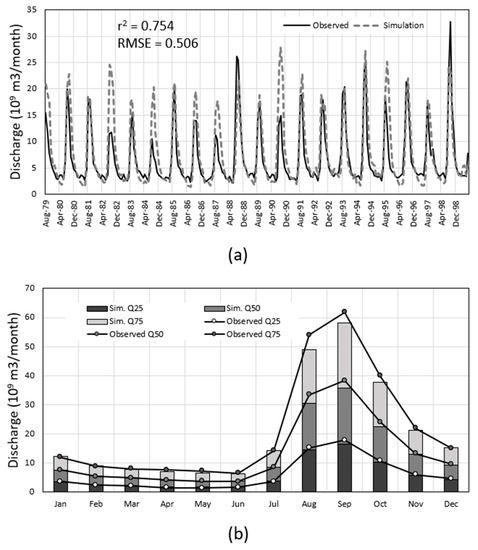
Figure 3.
(a) Comparison of the simulated and the observed time series from August 1979 to July 1999 of one trial using the Pearson III distribution for the Nile River; (b) comparison between observed and simulated iteration’s monthly discharge quartiles using the Pearson III distribution for the Nile River.
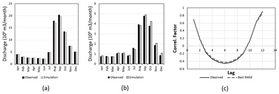

Figure 4.
(a) Comparison of the monthly mean using Pearson III distribution for the Nile River; (b) comparison of the standard deviation; (c) autocorrelation (Lag 1 to 12) comparison for 100 iterations; (d) coefficient of determination comparison for 100 iterations; (e) root mean square error comparison for 100 iterations; (f) Kling–Gupta efficiency coefficient; (g) Nash–Sutcliffe efficiency coefficient.
On the other hand, Figure 5 and Figure 6 show the simulated discharge results for the Nile River using randomized Fourier transformation. Figure 5b shows a comparison between observed and simulated monthly quartiles (25, 50, and 75 quartiles) of discharge for this iteration. The results confirmed that the model could accurately capture the monthly variation in discharge during low-flow months (November to July). The figure also shows that the result of the simulated flow during the flood time is slightly better than the previous model.
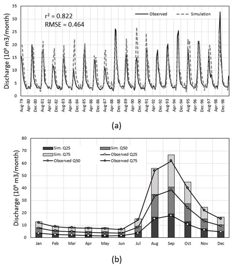
Figure 5.
(a) Comparison of the simulated and the observed time series from August 1979 to July 1999 using DFT for the Nile River; (b) comparison between observed and simulated monthly discharge quartiles using DFT for the Nile River.
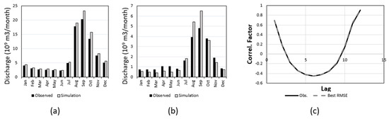
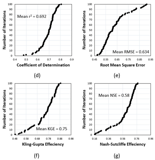
Figure 6.
(a) Comparison of the monthly mean using DFT distribution for the Nile River; (b) comparison of the standard deviation; (c) autocorrelation (lag 1 to 12) comparison for 100 iterations; (d) coefficient of determination comparison for 100 iterations; (e) root mean square error comparison for 100 iterations; (f) Kling–Gupta efficiency coefficient; (g) Nash–Sutcliffe efficiency coefficient.
Figure 7 compares the cumulative probability distributions of the discharges from the two simulations with the observed discharge for the Nile River in Figure 7a (March) (representing the low flow) and Figure 7b (September) (representing the flood period). The findings demonstrate that with a slightly larger discharge during the flood period, the two models could rather accurately mimic the observed discharge.
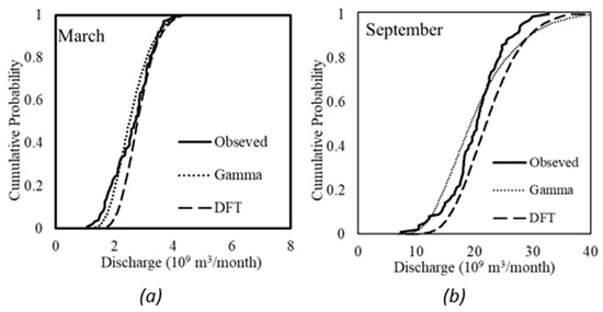
Figure 7.
Comparison of the cumulative probability distributions of the two models and the measured discharge for the Nile River in (a) March and (b) September.
5. Discussion
The results indicate that the proposed approach can be useful for constructing synthetic models that statistically represent the observed dataset. It also displayed a high level of versatility and modularity owing to its simplistic architecture. Unlike models commonly used for stochastic generation of streamflow time series, such as ARMA models, the simulation approach presented here reproduces both short- and long-range dependence. On the other hand, although machine learning techniques showed acceptable results, they are considered “black box” techniques.
Several studies have been performed using FT analysis. Some of these models apply the FT as a single model without normalizing the data or removing the seasonal component, such as Chong et al. [28]. However, the results were not satisfactory, and they found that WT is more suitable than the FT model.
Other methods applied the FT in conjunction with statistical techniques, such as Anderson et al. [33] who developed the Fourier–PARMA model; Saremi et al. [57], who examined the performance and results of three different Fourier-based models and found that the three models were suitable for the modeling of dynamic streamflow time series; and Brunner et al. [29] who incorporated the flexible four-parameter kappa distribution with FT and found that the results were satisfactory. Comparing the results with current work is difficult due to the differences in flow characteristics in each river.
However, in all FT models including the current model, the portrayal of its dependency is limited to ranges within the duration of the observed time series. Another limitation of this approach is the requirement for a continuous original dataset with as few missing values as possible because the quality of the outcomes is strongly correlated with the size of the available data. Another limitation is that the approach assumes a strong cross-correlation between the explanatory variable (time) and the response variable (streamflow). A weak cross-correlation indicates the presence of external factors that influence the response variable.
Water resource uncertainties frequently result from the random behavior of hydrological processes and the limited historical data used to estimate the parameters of stochastic models [58]. Even though the 100-year Nile River streamflow data is believed to be sufficient to decrease the uncertainty error, the historical streamflow measurement, and recording accuracy may be the main source of uncertainty in this study.
Since the created model supports a flexible dependency structure that reflects the statistics of the observed data, it may be applied to any time series of river flows. The findings of this study ought to be helpful to professionals who want to produce high-resolution synthetic river flows for planning water resource systems, operations analysis, and flood and drought prediction.
6. Conclusions
The conclusions of this research may be summarized as follows:
- The investigated technique is a simple and modular method to generate synthetic time series data while maintaining (preserving) the statistics of the original dataset;
- An autoregressive time series decomposition is used for isolating the stochastic component of the original time series. Two stochastic analysis approaches are then used to construct a collection of surrogate time series. The first approach is based on the probability distribution of the data, while the second approach transfers the time series from the time domain into the frequency domain. The results of both approaches are good, as they accurately depicted the original data;
- Contradictory to previous research, the investigated technique is simple and does not require complex computations. It is advised to consider these aspects when handling datasets containing severe occurrences or affected by external variables other than the temporal one. It is also suggested to replace or include calculation steps regarding the system design;
- The proposed technique may be applied in various applications. It may be used to estimate missing data, predict hydrological time series for transboundary rivers, and resolve disputes in data-sharing disagreements among riparian countries. Therefore, it may have significant impacts in the field of water resources engineering.
Author Contributions
Conceptualization, A.M.E. and S.A.; methodology, S.A.; software, A.M.M.A.; validation, S.A.; formal analysis, S.A. and A.M.M.A.; investigation, S.A. and A.M.M.A.; resources, A.M.I.A.E. and A.M.E.; data curation, S.A.; writing—original draft preparation, A.M.M.A.; writing—review and editing, S.A. and A.M.I.A.E.; visualization, S.A. and A.M.M.A.; supervision, A.M.E., S.A. and A.M.I.A.E.; project administration, A.M.E.; funding acquisition, S.A. All authors have read and agreed to the published version of the manuscript.
Funding
This research received no external funding.
Institutional Review Board Statement
Not applicable.
Informed Consent Statement
Not applicable.
Data Availability Statement
The data that support the findings of this study are available on request from the corresponding author, (A.M.M.A.). The data are not publicly available due to the use of software developed by the authors.
Conflicts of Interest
The authors declare no conflict of interest.
References
- Borgomeo, E.; Farmer, C.L.; Hall, J.W. Numerical rivers: A synthetic streamflow generator for water resources vulnerability assessments. Water Resour. Res. 2015, 51, 5382–5405. [Google Scholar] [CrossRef]
- Silva, A.T.; Portela, M.M. Generation of monthly synthetic streamflow series based on the method of fragments. WIT Trans. Ecol. Environ. 2011, 145, 237–247. [Google Scholar]
- McAfee, S.A.; Pederson, G.T.; Woodhouse, C.A.; McCabe, G.J. Application of synthetic scenarios to address water resource concerns: A management-guided case study from the Upper Colorado River Basin. Clim. Serv. 2017, 8, 26–35. [Google Scholar] [CrossRef]
- de Almeida Pereira, G.A.; Veiga, Á. Periodic copula autoregressive model designed to multivariate streamflow time series modelling. Water Resour. Manag. 2019, 33, 3417–3431. [Google Scholar] [CrossRef]
- Pender, D.; Patidar, S.; Pender, G.; Haynes, H. Stochastic simulation of daily streamflow sequences using a hidden Markov model. Hydrol. Res. 2016, 47, 75–88. [Google Scholar] [CrossRef]
- Tedla, M.G.; Rasmy, M.; Tamakawa, K.; Selvarajah, H.; Koike, T. Assessment of Climate Change Impacts for Balancing Transboundary Water Resources Development in the Blue Nile Basin. Sustainability 2022, 14, 15438. [Google Scholar] [CrossRef]
- Nassar, G.; Amin, D.; Abdelaziz, S.; Youssef, T. Flow Forecasting and Skill Assessment in the Blue Nile Basin. Nile Water Sci. Eng. J. 2017, 10, 29. [Google Scholar]
- Herman, J.D.; Zeff, H.B.; Lamontagne, J.R.; Reed, P.M.; Characklis, G.W. Synthetic drought scenario generation to support bottom-up water supply vulnerability assessments. J. Water Resour. Plan. Manag. 2016, 142, 04016050. [Google Scholar] [CrossRef]
- Adhikary, S.K.; Rahman, M.; Gupta, A.D. A stochastic modelling technique for predicting groundwater table fluctuations with time series analysis. Int. J. Appl. Sci. Eng. Res. 2012, 1, 238–249. [Google Scholar]
- Wang, H.R.; Wang, C.; Lin, X.; Kang, J. An improved ARIMA model for precipitation simulations. Nonlinear Process. Geophys. 2014, 21, 1159–1168. [Google Scholar] [CrossRef]
- Montanari, A.; Rosso, R.; Taqqu, M.S. Fractionally differenced ARIMA models applied to hydrologic time series: Identification, estimation, and simulation. Water Resour. Res. 1997, 33, 1035–1044. [Google Scholar] [CrossRef]
- Kajuru, J.Y.; Abdulkarim, K.; Muhammed, M.M. Forecasting Performance of Arima and Sarima Models on Monthly Average Temperature of Zaria, Nigeria. ATBU J. Sci. Technol. Educ. 2019, 7, 205–212. [Google Scholar]
- Elganiny, M.A.; Eldwer, A.E. Comparison of stochastic models in forecasting monthly streamflow in rivers: A case study of River Nile and its tributaries. J. Water Resour. Prot. 2016, 8, 143–153. [Google Scholar] [CrossRef]
- Mohamed, T.M. Forecasting of Monthly Flow for the White Nile River (South Sudan). Am. J. Water Sci. Eng. 2021, 7, 103–112. [Google Scholar] [CrossRef]
- Sharma, A.; Tarboton, D.G.; Lall, U. Streamflow simulation: A nonparametric approach. Water Resour. Res. 1997, 33, 291–308. [Google Scholar] [CrossRef]
- Stedinger, J.R.; Taylor, M.R. Synthetic streamflow generation: 1. Model verification and validation. Water Resour. Res. 1982, 18, 909–918. [Google Scholar] [CrossRef]
- Koutsoyiannis, D. A generalized mathematical framework for stochastic simulation and forecast of hydrologic time series. Water Resour. Res. 2000, 36, 1519–1533. [Google Scholar] [CrossRef]
- Salas, J.D. Analysis and modelling of hydrological time series. In Handbook of Hydrology; McGraw-Hill, Inc.: New York, NY, USA, 1993; p. 19. [Google Scholar]
- Pathak, P. Developing a Synthetic Continuous Daily Streamflow Hydrograph Technique for Maryland; University of Maryland: College Park, MD, USA, 2005. [Google Scholar]
- Al-Alati, H.; Abdelaziz, S.; Gad, M. Markov Chain Time Series Analysis of Soil Water Level Fluctuationsin Jaber Al-Ahmadwetlandarea, Kuwait. Int. J. Mod. Eng. Res. (IJMER) 2018, 8, 17–28. Available online: https://www.ijmer.com (accessed on 17 September 2019).
- Prairie, J.; Nowak, K.; Rajagopalan, B.; Lall, U.; Fulp, T. A stochastic nonparametric approach for streamflow generation combining observational and paleoreconstructed data. Water Resour. Res. 2008, 44, W06423. [Google Scholar] [CrossRef]
- Mehrotra, R.; Sharma, A. A nonparametric stochastic downscaling framework for daily rainfall at multiple locations. J. Geophys. Res. Atmos. 2006, 111, D15. [Google Scholar] [CrossRef]
- Londhe, S.; Charhate, S. Comparison of data-driven modelling techniques for river flow forecasting. Hydrol. Sci. J.–J. Des Sci. Hydrol. 2010, 55, 1163–1174. [Google Scholar] [CrossRef]
- Boisvert, J.; El-Jabi, N.; St-Hilaire, A.; el Adlouni, S.-E. Parameter estimation of a distributed hydrological model using a genetic algorithm. Open J. Mod. Hydrol. 2016, 6, 151–167. [Google Scholar] [CrossRef]
- Khan, S.; Ganguly, A.R.; Saigal, S. Detection and predictive modeling of chaos in finite hydrological time series. Nonlinear Process. Geophys. 2005, 12, 41–53. [Google Scholar] [CrossRef]
- Lange, H.; Brunton, S.L.; Kutz, J.N. From Fourier to Koopman: Spectral Methods for Long-term Time Series Prediction. J. Mach. Learn. Res. 2021, 22, 1–38. [Google Scholar]
- Tangborn, A. Wavelet Transforms in Time Series Analysis; Global Modeling and Assimilation Office, Goddard Space Flight Center: Washington, WA, USA, 2010; pp. 1–31. [Google Scholar]
- Chong, K.L.; Lai, S.H.; El-Shafie, A. Wavelet transform based method for river stream flow time series frequency analysis and assessment in tropical environment. Water Resour. Manag. 2019, 33, 2015–2032. [Google Scholar] [CrossRef]
- Brunner, M.I.; Bárdossy, A.; Furrer, R. Stochastic simulation of streamflow time series using phase randomization. Hydrol. Earth Syst. Sci. 2019, 23, 3175–3187. [Google Scholar] [CrossRef]
- Wang, W.; Ding, J. Wavelet network model and its application to the prediction of hydrology. Nat. Sci. 2003, 1, 67–71. [Google Scholar]
- Fleming, S.W.; Marsh Lavenue, A.; Aly, A.H.; Adams, A. Practical applications of spectral analysis to hydrologic time series. Hydrol. Process. 2002, 16, 565–574. [Google Scholar] [CrossRef]
- Coulibaly, P.; Burn, D.H. Wavelet analysis of variability in annual Canadian streamflows. Water Resour. Res. 2002, 40, 1–14. [Google Scholar] [CrossRef]
- Anderson, P.L.; Tesfaye, Y.G.; Meerschaert, M.M. Fourier-PARMA models and their application to river flows. J. Hydrol. Eng. 2007, 12, 462–472. [Google Scholar] [CrossRef]
- Awadallah, A.G. Evolution of the Nile River drought risk based on the streamflow record at Aswan station, Egypt. Civ. Eng. Environ. Syst. 2014, 31, 260–269. [Google Scholar] [CrossRef]
- Shakweer, A.; Youssef, R.M. Futures studies in Egypt: Water foresight 2025. Foresight 2007, 9, 22–32. [Google Scholar] [CrossRef]
- Mohie El Din, M.O.; Moussa, A.M.A. Water management in Egypt for facing the future challenges. J. Adv. Res. 2016, 7, 403–412. [Google Scholar]
- Eid, H.M.; El-Marsafawy, S.M.; Ouda, S.A. Assessing the economic impacts of climate change on agriculture in Egypt: A Ricardian approach. In World Bank Policy Research Working Paper; The World Bank: Washington, DC, USA, 2007; p. 4293. [Google Scholar]
- Strzepek, K.M.; Yates, D.N. Responses and thresholds of the Egyptian economy to climate change impacts on the water resources of the Nile River. Clim. Chang. 2000, 46, 339–356. [Google Scholar] [CrossRef]
- Lotfy, W.M. Climate change and epidemiology of human parasitosis in Egypt: A review. J. Adv. Res. 2014, 5, 607–613. [Google Scholar] [CrossRef] [PubMed]
- Jungudo, M.M. The Impact of Climate Change in Egypt; Whitehead Morris Press: Cairo, Egypt, 2022; Volume 9, pp. 274–290. [Google Scholar]
- Nakhla, D.A.; Hassan, M.G.; el Haggar, S. Impact of biomass in Egypt on climate change. Nat. Sci. 2013, 05, 678–684. [Google Scholar] [CrossRef]
- Sharaan, M.; Iskander, M.; Udo, K. Coastal adaptation to Sea Level Rise: An overview of Egypt’s efforts. Ocean Coast. Manag. 2022, 218, 106024. [Google Scholar] [CrossRef]
- Shoup, J.A. The Nile: An Encyclopedia of Geography, History, and Culture; ABC-CLIO: Santa Barbara, CA, USA, 2017; Available online: https://books.google.co.uk/books?id=ZXCrDgAAQBAJ (accessed on 18 September 2019).
- Melesse, A.M.; Abtew, W.; Setegn, S.G. Nile River Basin; Springer: Berlin/Heidelberg, Germany, 2011. [Google Scholar]
- El-Kammash, M.; Smith, C.; Hurst, H. Nile River; Encyclopedia Britannica: Chicago, IL, USA, 2022. [Google Scholar]
- Koutsoyiannis, D.; Yao, H.; Georgakakos, A. Medium-range flow prediction for the Nile: A comparison of stochastic and deterministic methods/Prévision du débit du Nil à moyen terme: Une comparaison de méthodes stochastiques et déterministes. Hydrol. Sci. J. 2008, 53, 142–164. [Google Scholar] [CrossRef]
- Hurst, H.E.; Phillips, P.; Black, R.P. The Nile Basin; Government Press: Nairobi, Kenya, 1961; Volume 4, Available online: https://books.google.se/books?id=WJt-AAAAMAAJ (accessed on 14 November 2019).
- Hurst, H.E. Second Supplement to Volume 3 of The Nile Basin: Ten-Day Mean and Monthly Mean Guage Readings of The Nile and Its Tributaries for the Years 1933–1937 and Normals for the Period 1912–1937; Whitehead Morris Press: Cairo, Egypt, 1939; Volume 3, Available online: https://books.google.se/books?id=bWLPzQEACAAJ (accessed on 18 September 2019).
- Karmeshu, N. Trend Detection in Annual Temperature Precipitation using the Mann Kendall Test-A Case Study to Assess Climate Change on Select States in the Northeastern United States. Master’s Thesis, University of Pennsylvania, Philadelphia, PA, USA, 2012. [Google Scholar]
- Langat, P.K.; Kumar, L.; Koech, R. Identification of the most suitable probability distribution models for maximum, minimum, and mean streamflow. Water 2019, 11, 734. [Google Scholar] [CrossRef]
- Helsel, D.R.; Hirsch, R.M.; Ryberg, K.R.; Archfield, S.A.; Gilroy, E.J. US Geological Survey. Statistical methods in water resources. In Techniques and Methods; US Geological Survey: Reston, VA, USA, 2020. [Google Scholar] [CrossRef]
- Stein, E.; Shakarchi, R. Fourier Analysis: An Introduction; Princeton University Press: Princeton, NJ, USA, 2003. [Google Scholar]
- Tolstov, G. Fourier Series; Dover Publications Inc.: New York, NY, USA, 1962. [Google Scholar]
- Venema, V.; Ament, F.; Simmer, C. A Stochastic Iterative Amplitude Adjusted Fourier Transform algorithm with improved accuracy. Nonlinear Process. Geophys. 2006, 13, 321–328. [Google Scholar] [CrossRef]
- Vrugt, J.A.; de Oliveira, D.Y. Confidence intervals of the Kling-Gupta efficiency. J. Hydrol. 2022, 612, 127968. [Google Scholar] [CrossRef]
- Zeybek, M. Nash-sutcliffe efficiency approach for quality improvement. J. Appl. Math. Comput. 2018, 2, 496–503. [Google Scholar] [CrossRef]
- Saremi, A.; Pashaki, M.H.K.; Sedghi, H.; Rouzbahani, A.; Saremi, A. Simulation of river flow using Fourier series models. In Proceedings of the International Conference on Environmental and Computer Science, Dubai, United Arab Emirates, 28–30 December 2009; Volume 19, p. 133. [Google Scholar]
- Lee, D.-J.; Salas, J.D.; Boes, D.C. Uncertainty Analysis for Synthetic Streamflow Generation. In Proceedings of the World Environmental and Water Resources Congress 2007, Tampa, Florida, 15–19 May 2007. [Google Scholar]
Disclaimer/Publisher’s Note: The statements, opinions and data contained in all publications are solely those of the individual author(s) and contributor(s) and not of MDPI and/or the editor(s). MDPI and/or the editor(s) disclaim responsibility for any injury to people or property resulting from any ideas, methods, instructions or products referred to in the content. |
© 2023 by the authors. Licensee MDPI, Basel, Switzerland. This article is an open access article distributed under the terms and conditions of the Creative Commons Attribution (CC BY) license (https://creativecommons.org/licenses/by/4.0/).