
Reducing Urban Traffic Congestion via Charging Price


Abstract
1. Introduction
2. Literature Review
3. Examples of Reducing Urban Traffic Congestion via Charging Price in City of Milan, Italy; City of London, England; City of Stockholm, Sweden; City of Singapore; and City of Teheran, Iran
3.1. London
3.2. Stockholm
3.3. Milan
3.4. Teheran
3.5. Singapore
4. Methodology of Analysis and Diagnostic
4.1. Design of the Survey and Sample Design
4.2. Data Analysis
4.3. Traffic Charging Zone
5. Multivariable Model
5.1. Regression versus Correlation
5.2. Characteristics of the Model
6. Result
6.1. Testing the Overall Significance of the Sample Regression
6.2. Testing the Overall Significance of a Multiple Regression in Terms of Coefficient of Correlation, ρ
6.3. Emissions Savings and Calculation of Environmental Decongestion
6.4. Savings in Noise Pollution Emissions
7. Discussion

| Santiago | |
|---|---|
| No. of inhabitants | 8,918,653 |
| No. of inhabitants in country or region | Country: 20.4 million |
| City area | 1485 km2 |
| Density | 6000/km2 |
| No. of vehicles/1000 Inhabitants | 230 vehicles |
| GDP per capita | USD 13,341 |
| TCO2 per capita | 4,6 |
| Kg CO2/USD 1000 | 0.17 |
| Type of system | Area. Fee to obtain a pass to enter the area, which can be per day |
| Rate to charge | USS 0.46 |
8. Conclusions
Author Contributions
Funding
Institutional Review Board Statement
Informed Consent Statement
Data Availability Statement
Acknowledgments
Conflicts of Interest
References
- Ford, B. Bill Ford Discusses a Future Beyond Traffic Gridlock. TEDtalk. 7 July 2011. Available online: https://www.ted.com/talks/bill_ford_a_future_beyond_traffic_gridlock (accessed on 17 March 2021).
- United Nations. The World’s Cities in 2016. Available online: http://www.un.org/en/development/desa/population/publications/pdf/urbanization/the_worlds_cities_in_2016_data_booklet.pdf (accessed on 23 April 2021).
- United Nations. Available online: https://www.un.org/development/desa/pd/sites/www.un.org.development.desa.pd/files/undes_pd_2020_popfacts_urbanization_policies.pdf (accessed on 15 December 2022).
- Growth in Urban Population Outpaces Rest of Nation, Census Bureau Reports. United States Census Bureau. 2021. Available online: https://www.census.gov/newsroom/press-releases/2021/public-transportation-commuters.html (accessed on 15 December 2022).
- Inrix. Global Traffic Scorecard Report. 2021. Available online: http://inrix.com/scorecard/ (accessed on 15 November 2022).
- Sotra, M. 7 Smart City Solutions to Reduce Traffic Congestion. 2017. Available online: https://www.geotab.com/blog/reduce-traffic-congestion/ (accessed on 17 September 2021).
- Cohn, N. Beat Congestion. Senior Traffic Expert at TomTom. 2016. Available online: https://www.tomtom.com/en_gb/trafficindex/beatcongestion (accessed on 15 May 2018).
- Mtc. Metropolitan Transportation Commission. 2018. Available online: https://mtc.ca.gov/ (accessed on 6 June 2022).
- Latimes. L.A.’s Traffic Congestion Is World’s Worst for Sixth Straight Year, Study Says. 2018. Available online: http://www.latimes.com/local/lanow/la-me-la-worst-traffic-20180206-story.html# (accessed on 6 February 2021).
- Tomtom Traffic Index. Measuring Congestion Worldwide. Available online: https://www.tomtom.com/traffic-index/santiago-traffic (accessed on 20 November 2022).
- London Congestion Charge: Why It’s Time to Reconsider One of the City’s Great Successes. 2 March 2018. Available online: https://theconversation.com/london-congestion-charge-why-its-time-to-reconsider-one-of-the-citys-great-successes-92478 (accessed on 20 July 2021).
- Magnanti, T.L.; Wong, R.T. Network Design and Transportation Planning: Models and Algorithms. Transp. Sci. 1984, 18, 1–55. [Google Scholar] [CrossRef]
- United Nations. Sustainable Development. Thematic Session 5: Policies for Sustainable Transport 16 October 2021. Available online: https://sdgs.un.org/events/thematic-session-5-policies-sustainable-transport-34334 (accessed on 10 November 2022).
- Hysing, E.; Isaksson, K. Building acceptance for congestion charges—The Swedish experiences compared. J. Transp. Geogr. 2015, 49, 52–60. [Google Scholar] [CrossRef]
- Dieplinger, M.; Fürst, E. The acceptability of road pricing: Evidence from two studies in Vienna and four other European cities. Transp. Policy 2014, 36, 10–18. [Google Scholar] [CrossRef]
- Glavic, D.; Mladenovic, M.; Luttinen, T.; Cicevic, S.; Trifunovic, A. Road to price: User perspectives on road pricing in transition country. Transp. Res. Part A 2017, 105, 79–94. [Google Scholar] [CrossRef]
- Pronello, C.; Rappazzo, V. Road pricing: How people perceive a hypothetical introduction. The case of Lyon. Transp. Policy 2014, 36, 192–205. [Google Scholar] [CrossRef]
- Lindsey, R. Road pricing and investment. Econ. Transp. 2012, 1, 49–63. [Google Scholar] [CrossRef]
- Zangui, M.; Yin, Y.; Lawphongpanich, S.; Chen, S. Differentiated Congestion Pricing of Urban Transportation Networks with Vehicle-Tracking Technologies. Procedia-Soc. Behav. Sci. 2013, 80, 289–303. [Google Scholar] [CrossRef]
- Sandholm, W.H. Evolutionary Implementation and Congestion Pricing. Rev. Econ. Stud. 2002, 69, 667–689. [Google Scholar] [CrossRef]
- Francke, A.; Kaniok, D. Responses to differentiated road pricing schemes. Transp. Res. Part A 2013, 48, 25–30. [Google Scholar] [CrossRef]
- Iseki, H.; Demisch, A. Examining the linkages between electronic roadway tolling technologies and road pricing policy objectives. Res. Transp. Econ. 2012, 36, 121–132. [Google Scholar] [CrossRef]
- Agyapong, F.; Ojo, T. Managing traffic congestion in the Accra Central Market, Ghana. J. Urban Manag. 2018, 7, 85–96. [Google Scholar] [CrossRef]
- Brent, D.A.; Gross, A. Dynamic road pricing and the value of time and reliability. J. Reg. Sci. 2017, 58, 330–349. [Google Scholar] [CrossRef]
- Gibson, M.; Carnovale, M. The effects of road pricing on driver behavior and air pollution. J. Urban Econ. 2015, 89, 62–73. [Google Scholar] [CrossRef]
- Cavallaro, F.; Giaretta, F.; Nocera, S. The potential of road pricing schemes to reduce carbon emissions. Transp. Policy 2018, 67, 85–92. [Google Scholar] [CrossRef]
- Coria, J.; Zhang, X.-B. Optimal environmental road pricing and daily commuting patterns. Transp. Res. Part B 2017, 105, 297–314. [Google Scholar] [CrossRef]
- Agarwal, S.; Koo, K.M. Impact of electronic road pricing (ERP) changes on transport modal choice. Reg. Sci. Urban Econ. 2015, 60, 1–11. [Google Scholar] [CrossRef]
- Buyukeren, A.C.; Hiramatsu, T. Anti-congestion policies in cities with public transportation. J. Econ. Geogr. 2015, 16, 395–421. [Google Scholar] [CrossRef]
- Percoco, M. The impact of road pricing on housing prices: Preliminary evidence from Milan. Transp. Res. Part A 2014, 67, 188–194. [Google Scholar] [CrossRef]
- Duque-Escoba, G. Toll Roads in Colombia Are Overexploited; Universidad Nacional de Colombia: Bogotá, Colombia, 2018; Available online: http://unperiodico.unal.edu.co/pages/detail/toll-roads-in-colombia-are-overexploited/ (accessed on 18 April 2022).
- Anas, A.; Timilsina, G. Impacts of Policy Instruments to Reduce Congestion and Emissions from Urban Transportation: The Case of São Paulo, Brazil1; The World Bank Development Research Group Environment and Energy Team: Washington, DC, USA, 2009. [Google Scholar]
- Croci, E. Urban Road Pricing: A Comparative Study on the Experiences of London, Stockholm and Milan. Transp. Res. Procedia 2016, 14, 253–262. [Google Scholar] [CrossRef]
- He, B.Y.; Zhou, J.; Ma, Z.; Wang, D.; Sha, D.; Lee, M.; Chow, J.Y.; Ozbay, K. A validated multi-agent simulation test bed to evaluate congestion pricing policies on population segments by time-of-day in New York City. Transp. Policy 2021, 101, 145–161. Available online: https://www.sciencedirect.com/science/article/abs/pii/S0967070X20309483#! (accessed on 15 November 2022). [CrossRef]
- Genser, A.; Kouvelas, A. Dynamic optimal congestion pricing in multi-region urban networks by application of a Multi-Layer-Neural network. Transp. Res. Part C Emerg. Technol. 2022, 134, 103485. Available online: https://www.sciencedirect.com/science/article/pii/S0968090X2100471X#! (accessed on 15 November 2022). [CrossRef]
- Zheng, L.; Liu, P.; Huang, H.; Ran, B.; He, Z. Time-of-day pricing for toll roads under traffic demand uncertainties: A distributionally robust simulation-based optimization method. Transp. Res. Part C Emerg. Technol. 2022, 144, 103894. [Google Scholar] [CrossRef]
- Visaria, A.; Jensen, A.; Thorhauge, M.; Mabit, S. User preferences for EV charging, pricing schemes, and charging infrastructure. Transp. Res. Part-A Policy Pract. 2022, 165, 120–143. Available online: https://www.webofscience.com%2fwos%2fauthor%2frecord%2f29795377 (accessed on 15 November 2022). [CrossRef]
- RaviSeshadri, A.; Ben-Akiva, M. Congestion tolling—Dollars versus tokens: Within-day dynamics. Transp. Res. Part C Emerg. Technol. 2022, 143, 103836. Available online: https://www.sciencedirect.com%2fscience%2farticle%2fpii%2fS0968090X2200256X%3fvia%253Dihub#! (accessed on 15 November 2022).
- Struyf, C.; Voorde, E.; Vanelslander, T. Calculating the cost of congestion to society: A case study application to Flanders. Res. Transp. Bus. Manag. 2022, 44, 100573. Available online: https://www.sciencedirect.com/science/article/abs/pii/S2210539520301115?via%3Dihub (accessed on 15 November 2022). [CrossRef]
- Ecola, L.; Light, T. Making Congestion Pricing Equitable. Transp. Res. Rec. J. Transp. Res. Board 2010, 2187, 53–59. Available online: https://journals.sagepub.com/doi/10.3141/2187-08 (accessed on 15 November 2022). [CrossRef]
- Schubert, D.; Sys, C.; Vanelslander, T.; Roumboutsos, A. No-queue road pricing: A comprehensive policy instrument for Europe? Util. Policy 2022, 78, 101413. Available online: https://www.sciencedirect.com/science/article/abs/pii/S0957178722000789?via%3Dihub (accessed on 15 November 2022). [CrossRef]
- Fageda, X.; Flores-Fillol, R.; Theilen, B. Price versus quantity measures to deal with pollution and congestion in urban areas: A political economy approach. J. Environ. Econ. Manag. 2022, 115, 102719. Available online: https://www.sciencedirect.com/science/article/pii/S0095069622000778?via%3Dihub (accessed on 15 November 2022). [CrossRef]
- Pattinson, J.-A.; Harrison, G.; Mullen, C.; Shepherd, S. Combining Tradable Credit Schemes with a New Form of Road Pricing: Producing Liveable Cities and Meeting Decarbonisation Goals. Sustainability 2022, 14, 8413. Available online: https://www.mdpi.com/2071-1050/14/14/8413 (accessed on 15 November 2022). [CrossRef]
- Datosmacro.com. Available online: https://datosmacro.expansion.com/paises/singapur (accessed on 8 November 2022).
- World Bank. Available online: https://datos.bancomundial.org/indicator/EN.ATM.CO2E.KD.GD?locations=SG (accessed on 8 November 2022).
- Singapore Government Agency Website. Available online: https://onemotoring.lta.gov.sg/content/onemotoring/home/driving/entering_and_exiting_singapore/cars-and-motorcycles-registered-in-malaysia.html#:~:text=Vehicles%20Entry%20Permit%20(VEP)%20Fees,Sundays%20and%20Singapore%20public%20holidays (accessed on 8 November 2022).
- City Populations Worldwide. Available online: http://poblacion.population.city/suecia/stockholm/ (accessed on 9 November 2022).
- Datosmacro.com. Available online: https://datosmacro.expansion.com/energia-y-medio-ambiente/emisiones-co2/suecia (accessed on 9 November 2022).
- Transport in Stockholm. Available online: https://www.transportstyrelsen.se/en/road/road-tolls/Congestion-taxes-in-Stockholm-and-Goteborg/congestion-tax-in-stockholm/hours-and-amounts-in-stockholm/ (accessed on 9 November 2022).
- Population.City. Available online: http://population.city/united-kingdom/london/ (accessed on 10 November 2022).
- Statista Statistic. Available online: https://www.statista.com/statistics/314980/licensed-cars-in-london-england-united-kingdom/ (accessed on 10 November 2022).
- London Energy and Greenhouse Gas Inventory (LEGGI). Available online: https://data.london.gov.uk/dataset/leggi (accessed on 10 November 2022).
- Transport of London. Available online: https://tfl.gov.uk/modes/driving/congestion-charge/congestion-charge-zone (accessed on 10 November 2022).
- Studocu, Universidad del Norte, Italia. Available online: https://www.studocu.com/ec/document/universidad-tecnica-del-norte/metodologia-de-la-investigacion/datos-sobre-milan-apuntes-1/21255417 (accessed on 11 November 2022).
- Economy of Milan. Available online: https://dbpedia.org/page/Economy_of_Milan (accessed on 11 November 2022).
- Worldbank. Available online: https://data.worldbank.org/indicator/EN.ATM.CO2E.PC?locations=IT (accessed on 11 November 2022).
- Urban Access Regulation in Europe. Available online: https://es.urbanaccessregulations.eu/countries-mainmenu-147/italy-mainmenu-81/lombardia/milan-area-c-charging-scheme (accessed on 11 November 2022).
- Britannica. Available online: https://www.britannica.com/place/Tehran (accessed on 12 November 2022).
- Trading Economics. Available online: https://tradingeconomics.com/iran/gdp-per-capita#:~:text=GDP%20per%20Capita%20in%20Iran%20is%20expected%20to%20reach%203500.00,according%20to%20our%20econometric%20models (accessed on 12 November 2022).
- Expansion. Available online: https://datosmacro.expansion.com/paises/iran (accessed on 12 November 2022).
- Tehran Traffic Congestion Charging Management. Available online: https://www.witpress.com/elibrary/wit-transactions-on-the-built-environment/128/23240 (accessed on 12 November 2022).
- Buntz, B. The World’s 5 Smartest Cities. 2016. Available online: http://www.iotworldtoday.com/2016/05/18/world-s-5-smartest-cities/ (accessed on 16 April 2022).
- Transport for London. Congestion Charge. Available online: https://tfl.gov.uk/corporate/transparency/ (accessed on 23 December 2021).
- Eliasson, J. How to Solve Traffic Jams. TED Talk. 2012. Available online: https://www.youtube.com/watch?v=CX_Krxq5eUI&t=39s (accessed on 23 July 2021).
- ECOPASS: El Sistema de Tarificación Vial de Milán. Available online: https://www.plataformaurbana.cl/archive/2010/05/26/ecopass-el-sistema-de-tarificacion-vial-de-milan/ (accessed on 16 November 2022).
- Thynell, M. Modernidad en Movimiento. Cómo Enfrentarse a la Movilidad Motorizada en Teherán, Santiago y Copenhague. Revista Eure, N° 94; Santiago de Chile, December 2005; Volume XXXI, pp. 55–77. Available online: https://www.scielo.cl/scielo.php?script=sci_arttext&pid=S0250-71612005009400004#9 (accessed on 5 November 2022).
- Agarwal, S.; Koo, K.M.; Sing, T.F. Impact of electronic road pricing on real estate prices in Singapore. J. Urban Econ. 2015, 90, 50–59. [Google Scholar] [CrossRef]
- Phang, S.Y.; Toh, R.S. Road congestion pricing in Singapore: 1975 to 2003. Transp. J. 2004, 43, 16–25. [Google Scholar]
- Canavos, G. Probabilidad y Estadística. Aplicaciones y Métodos; McGraw-Hill, Interamerica de Mexico: Mexico city, Mexico, 1998. [Google Scholar]
- Morgenstern, O. The Accuracy of Economic Observations, 2nd ed.; Princeton University Press: Princeton, NJ, USA, 1963. [Google Scholar]
- OECD Social and Welfare Statistics: Income Distribution. 2017. Available online: https://data.oecd.org/inequality/income-inequality.htm (accessed on 1 January 2022).
- Gleave, S. Tarificación Vial por Congestión para la Ciudad de Santiago de Chile; Programa de las Naciones Unidas para el Desarrollo: Vitacura, Chile, 2019. [Google Scholar]
- Dönicke, D.B.; Lanyon, F.R.; Del Bío-Bío, U. Cálculo del consumo de combustible y emisiones De co2 de camiones mineros, mediante simulación Discreta. Rev. Ingeneria Ind. 2017, 16, 151–168. [Google Scholar] [CrossRef] [PubMed]
- Avance de Emisiones de Gases de Efecto Invernadero Correspondientes al Año 2021. Ministerio para la Transición Ecológica y el Reto Demográfico; Technical Report; Ministerio Para la Transición Ecológica y el Reto Demográfico: Madrid, Spain, 2022. [Google Scholar]
- Contaminación Acústica de los Vehiculos. Available online: https://tuteorica.com/material-complementario/contaminacion-acustica-de-los-vehculos/ (accessed on 14 November 2022).
- Crotte, A.; Garduño, J.; Arvizu, C. Tarificación Vial: Una Política para la Reducción de Externalidades Negativas Producidas por el Congestionamiento Vial, Financiado por el BID en 2018; IDB: Washington, DC, USA, 2018. [Google Scholar]
- Lopez, R.; Bocarejo, J.P. Políticas de Tarificación por Congestión: Efectos Potenciales y Consideraciones para su Implementación en Bogotá, Ciudad de México y Santiago; Banco Interamericano de Desarrollo: Washington, DC, USA, 2018. [Google Scholar] [CrossRef]
- Generadoras de Chile. Available online: http://generadoras.cl/generacion-electrica-en-chile (accessed on 15 November 2022).
- Statista. Available online: https://www.statista.com/statistics/952800/main-means-transport-chile/ (accessed on 23 November 2022).
- Greene, M.; Mora, R. Las Autopistas Urbanas Concesionadas: Una Nueva Forma de Segregación. Revista ARQ (Santiago). 2005. Available online: http://www.scielo.cl/pdf/arq/n52/art18 (accessed on 1 August 2022).


| Author | Methodology/Method | Description | Study Case |
|---|---|---|---|
| [34] | Multi-agent simulation model | Evaluation of congestion pricing policies in hourly population segments in New York City. The work presented here differs from the New York study in that the segmentation is by time slots. | New York City |
| [35] | Multilayer neural network model | Assessment of dynamic pricing in large-scale urban networks aiming at transport balances. | Zurich, Switzerland, |
| [36] | Simulation-based optimization model | The work evaluates where and how much to charge, under the uncertainties of origin-to-destination traffic demand, and through a set of probability distributions. | Anaheim network |
| [37] | Mixed logistic models applied to 558 electric vehicles | Analyses of user preferences related to electric vehicle (EV) charging decisions. The design declared two experiments. The first analyzed long-term decisions related to regular loading practices. The second captures decisions related to occasional cargo needs on longer trips. | Denmark, Finland, Iceland, Norway, and Sweden, |
| [38] | Mixed logistic and supply model for static congestion. | The work proposes a revolving credit scheme as an alternative to congestion charges. It studies the impact of sales behavior on the performance of the credit system. It models travel demand by using a mixed logistic and supply model on static congestion. | Denmark, France, Usa |
| [39] | Transport Cost Modes Model | It calculates the impact of congestion on operational and social costs. A meeting of experts used the literature’s relevant concepts to develop a proprietary instrument for the calculation of congestion costs that was applied and validated in a specific congestion situation. Results tested the effect of congestion mitigation measures (e.g., road pricing). | Flanders, Belgium |
| [40] | Equitable costing model | This document identifies and evaluates ways to make congestion pricing equitable. The authors review the equity notion applicable to congestion pricing. It explores equity issues that arise in restricted areas, charging systems, and high-occupancy toll lanes. | Los Angeles, USA |
| [41] | NQRP economic evaluation models | This paper reviews the literature to demonstrate the potential of no-queue road pricing (NQRP). It aims at establishing tolls that respond to traffic conditions in real time and addresses three challenges, namely congestion management, projects investment prioritization, and sustainable road financing. It examines the limitations of NQRP and the reasons why it does not have implementations in Europe. | European countries |
| [42] | Linear regression | This paper explores how to mitigate pollution and congestion in urban areas by adopting mechanisms based on price or quantity. The proposed model analysis has the predominance of quantity schemes over price schemes. It also explains traffic restrictions, such as the implementation of hybrid price and quantity systems. | Large cities in European countries such as Berlin, Hamburg, Munich, Brussels, Milan, Rome, Paris, London, or Madrid. |
| [43] | Semi structured interview method to experts | It analyzes a tradable credit scheme operation (TCS), which aims to reduce road traffic and contribute to livable cities and climate-change promises. The study uses qualitative methods, including semi-structured interviews with experts and stakeholders, as well as a review of the literature and documents. Based on the results, it proposes a new TCS form to keep government revenues, which will encourage road users to reduce kilometers traveled, reducing pollution and congestion. | United Kingdom |
| Singapore [44,45,46] | Stockholm [47,48,49] | London [50,51,52,53] | Milan [54,55,56,57] | Tehran [58,59,60,61] | |
|---|---|---|---|---|---|
| No. of inhabitants | 5,454,000 | 912,000 | 9498.212 | 1,396,522 | 8,693,706 |
| No. of inhabitants Country or region | 5,454,000 | Region: 1,057,120 | Country: 67,651,228 | Region: 3,775,765 | Region: 15,232,564 |
| City area | 728 km2 | 381.63 km2 | 1572 km2 | 1982 km2 | 707 km2 |
| Density | 7720 hab./km2 | 3597 hab./km2 | 5518 hab./km2 | 7400 hab./km2 | 12,296 hab./km2 |
| No. of vehicles/1000 inhabitants | 146 vehicles | 543 vehicles | 2600 vehicles | 679 vehicles | 4000 vehicles |
| GDP per capita | USD 61,507 | USD 50,050 (EUR 51,560) | 68,510.22 USD (GBP 55,974) | USD 55,600 | USD 5333.05 |
| TCO2 per capita | 9.71 ton | 3.82 ton | 3.5 ton | 5.45 ton | 8.43 ton |
| Kg CO2/USD 1000 | 0.10 kg CO2 | 0.07 kg CO2 | 0.11 kg CO2 | 0.13 kg CO2 | 0.54 kg CO2 |
| Type of System | It was the first city to successfully implement ERP electronic toll, charged to all vehicles entering and leaving the urban center. | Two areas, fixed rates when entering and leaving from Monday to Friday from 6:30 a.m. to 6:30 p.m. | Area. Fixed rate per day with unlimited entries and exits to the charged zone. | Area. Fixed rate depending on the type of user. Eco pass paid based on gases emission. | Area. Fee to obtain a pass to enter the area, which can be per day. |
| Charged rate | Collection is through a card; daily charges are USD 3.3 for residents and USD 35 for non-residents. | Between EUR 1.19 and 3.24 per crossing. EUR 11 per day maximum. | GBP 15. Electronic payment. | Non-residents (EUR 5), residents (EUR 2), commercial vehicles (EUR 3). | (USD 11.5) per week, (USD 70) per month or (USD 174) per year. |
| Variable | Observations | Minimum Price | Maximum Price | Average | Standard Deviation |
|---|---|---|---|---|---|
| Price | 500 | 200 | 1000 | 400 | 247.60 |
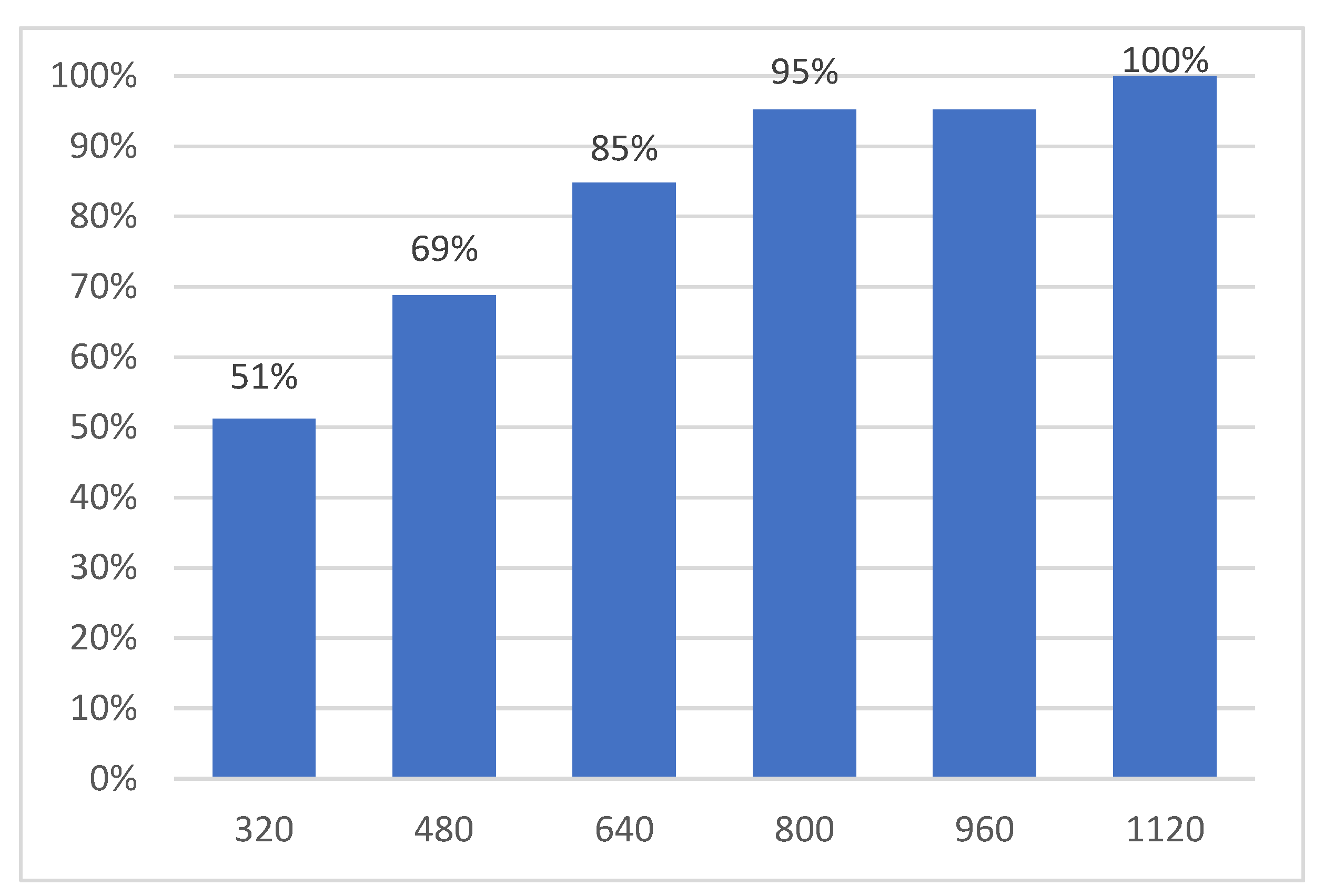
| Lower Limit (CLP) | Upper Limit (CLP) | Frequency (Drivers) | Payment Probability |
|---|---|---|---|
| 160 | 320 | 256 | 51.2% |
| 320 | 480 | 88 | 17.6% |
| 480 | 640 | 80 | 16.0% |
| 640 | 800 | 52 | 10.4% |
| 800 | 960 | 0 | 0.00% |
| 960 | 1120 | 24 | 4.80% |
| Source | Value | Average (Price) |
|---|---|---|
| Interception | 381.818 | |
| South | −127.273 | 254.545 |
| East | 157.312 | 539.130 |
| North | 127.273 | 509.091 |
| West | 103.896 | 458.714 |
| Zones | Level of Difficulty of Arrival at the Center | Average Distance in Kilometers to the Center | Weight by Distance in Kilometers | Average Weight |
|---|---|---|---|---|
| North | 30% | 17 | 23% | 27% |
| East | 13% | 13.2 | 18% | 15% |
| Center | 2% | 2 | 3% | 2% |
| South | 30% | 25 | 34% | 32% |
| West | 25% | 16.5 | 22% | 24% |
| 100% | 73.7 | 100% | 100% |
| Source | Value |
|---|---|
| South | −0.247 |
| North | 0.230 |
| East | 0.478 |
| West | 0.129 |
| Source | GL | Sum of Squares | Mean Squares | F | Pr > F | R2 |
|---|---|---|---|---|---|---|
| Model (MSS) | 4 | 6,992,298.137 | 1,748,074.534 | 36.966 | 0.0001 | 0.230 |
| Error (ESS) | 495 | 23,407,701.863 | 47,288.287 | |||
| Total | 499 | 30,400,000.000 |
| Concept | Unit | Savings per Pass | Savings Assuming 100 Passes per Year |
|---|---|---|---|
| 75.52% CO2 emission savings | TonCO2 e. | 3768.93 | 376,893 |
| 15.08% CH4 emission savings (t) | TonCO2 e. | 752.588 | 75,258.8 |
| 7.27% N2O gas savings | TonCO2 e. | 362.819 | 36,281.9 |
| 2.13% other gases (HFCs + PFCs + SF6) savings | TonCO2 e. | 10.630 | 1063.00 |
| GHG total emission savings = CO2 + CH4 + N2O + other gases (HFCs + PFCs + SF6) | TonCO2 e. | 4894.967 | 489,496.7 |
| Average Weight | Average Distance in Kilometers to the Center Zones | Km by Area | Fuel Liters Saved per Vehicle (Approximately 10 Km per Liter) | Kg CO2 Emission Saving per Vehicle | Total Savings per Ton CO2 Considering the Total Number of Vehicles (3,489,750) | |
|---|---|---|---|---|---|---|
| North | 27% | 17 | 4.59 | 0.459 | 1.2393 | 4,324,847 |
| East | 15% | 13.2 | 1.98 | 0.198 | 0.5346 | 1,865,620 |
| Center | 2% | 2 | 0.04 | 0.004 | 0.0108 | 37,689 |
| South | 32% | 25 | 8 | 0.8 | 2.16 | 7,537,860 |
| West | 24% | 16.5 | 3.96 | 0.396 | 1.0692 | 3,731,241 |
| Ton CO2 saved | 17,497,258 | |||||
| Concept | Unit | |
|---|---|---|
| 75.52% CO2 emission savings | TonCO2 e. | 17,497,258 |
| 15.08% CH4 emission savings (t) | TonCH4 e. | 3,493,890 |
| 7.27% Gas N2O saving | TonN2O e. | 1,684,389 |
| 2.13% Other gases savings (HFCs + PFCs + SF6) | Ton (HFCs + PFCs + SF6) 2.13%.e. | 493,500 |
| Total emission savings of GHG = CO2 + CH4 + N2O + other gases (HFCs + PFCs + SF6) | Ton GHC e. | 23,169,038 |
Disclaimer/Publisher’s Note: The statements, opinions and data contained in all publications are solely those of the individual author(s) and contributor(s) and not of MDPI and/or the editor(s). MDPI and/or the editor(s) disclaim responsibility for any injury to people or property resulting from any ideas, methods, instructions or products referred to in the content. |
© 2023 by the authors. Licensee MDPI, Basel, Switzerland. This article is an open access article distributed under the terms and conditions of the Creative Commons Attribution (CC BY) license (https://creativecommons.org/licenses/by/4.0/).
Share and Cite
González-Aliste, P.; Derpich, I.; López, M. Reducing Urban Traffic Congestion via Charging Price. Sustainability 2023, 15, 2086. https://doi.org/10.3390/su15032086
González-Aliste P, Derpich I, López M. Reducing Urban Traffic Congestion via Charging Price. Sustainability. 2023; 15(3):2086. https://doi.org/10.3390/su15032086
Chicago/Turabian StyleGonzález-Aliste, Pablo, Iván Derpich, and Mario López. 2023. "Reducing Urban Traffic Congestion via Charging Price" Sustainability 15, no. 3: 2086. https://doi.org/10.3390/su15032086
APA StyleGonzález-Aliste, P., Derpich, I., & López, M. (2023). Reducing Urban Traffic Congestion via Charging Price. Sustainability, 15(3), 2086. https://doi.org/10.3390/su15032086