Article

State of Health Estimation of Lithium-Ion Batteries in Electric Vehicles Based on Regional Capacity and LGBM

1
National Engineering Laboratory for Electric Vehicles, Beijing Institute of Technology, Beijing 100081, China
2
Collaborative Innovation Center for Electric Vehicles in Beijing, Beijing Institute of Technology, Beijing 100081, China
*
Author to whom correspondence should be addressed.
Sustainability 2023, 15(3), 2052; https://doi.org/10.3390/su15032052
Submission received: 14 December 2022 / Revised: 16 January 2023 / Accepted: 17 January 2023 / Published: 21 January 2023
(This article belongs to the Section Energy Sustainability)

Abstract

:
Battery state of health (SOH) estimation is a prerequisite for battery health management and is vital for second-life utilization. Existing techniques implemented in well-controlled experimental conditions fail to reflect complex working conditions during actual vehicular operation. In this article, a novel SOH estimation method for battery systems in real-world electric vehicles (EVs) is presented by combing results of regional capacity calculation and a light gradient boosting machine (LGBM) model. The LGBM model is used to capture the relationship between battery degeneration and influential factors based on datasets from real-world EVs. The regional capacity, which is calculated through incremental capacity analysis with a Gaussian smoothing filter, is utilized to reflect the battery degradation level while ensuring high flexibility and applicability. Accumulated mileage, average charging current, average charging temperature, and start and end of SOC values are chosen as influential factors for model establishment. The effectiveness, complexity, superiority, and robustness of the proposed method are verified using data from real-world EVs. Results indicate accurate SOH estimation can be achieved with an average absolute error of only 0.89 Ah, where the MAPE and RMSE of the test vehicles are 2.049% and 1.153%, respectively.

1. Introduction

Air pollution and greenhouse gas emissions generated from fossil fuel-based transportation have drawn extensive attention [1,2]. Ecologically friendly technologies, particularly those on electric vehicles (EVs), have been greatly progressing and are promising to mitigate greenhouse gas emissions as well as to improve air quality [3,4,5]. Thanks to superiority in energy density and lifespan, lithium-ion batteries are pervasively applied in EVs [6,7,8]. However, performance degradation of lithium-ion batteries is inevitable [9]. It is generally believed that lithium-ion batteries reach their end of life when the capacity declines to 80% of the initial value and/or the internal resistance doubles. At that point, batteries are still appropriate for other applications such as electric bicycles, energy storage systems, etc. [10]. To ensure safe, reliable, and efficient operation of batteries in EVs and in second-life utilization, their state of health (SOH) must be precisely estimated, which constitutes a core functionality of a battery management system (BMS) [11].
Generally, the SOH can be defined by the ratio of parameters of an aged battery to its pristine values at the beginning of life [12]. On top of this idea, extensive studies have been carried out for SOH estimation, where three categories of methods have been proposed, namely experimental methods, model-based methods, and data-driven methods [13]. Experimental methods are established based on test data to analyze battery aging behaviors to realize SOH estimation [14]. For example, the Coulomb counting method calculates capacity by integrating charge transferred through a battery during a full charge/discharge process and links usable capacity to the SOH [15]. Similarly, the electrochemical impedance spectroscopy (EIS) method applies a sinusoidal signal to the battery to measure battery impedance in a very wide frequency range so that the SOH can be obtained through the relationship between resistance and battery aging level [16,17]. The major limitation of these methods is that they require stringent experimental conditions and high-precision experimental equipment, which are difficult to apply in real operational scenarios.
Model-based methods employ electrochemical models (EMs), equivalent circuit models (ECMs), or other types of models to simulate battery behaviors so that deterioration of performance can be captured. In this case, the problem of SOH estimation can be transferred to identifications of aging parameters [18]. For example, EMs use partial differential equations and algebraic equations to delineate battery dynamic performance to describe battery aging [19,20]. Despite high accuracy and physical interpretation ability, EMs are usually restricted from real-time implementations due to high computational burden. To reduce complexity, ECMs employing basic circuit components to simulate battery behaviors have been introduced [21,22], where various optimization and filtering algorithms are applied, including least squares (LS) [23], the Kalman filter (KF) [24], and the particle filter (PF) [25], to identify the characteristic parameters that can be related to SOH. Although the computational complexity is lower, methods of this type are susceptible to accuracy problems and have limited robustness to disturbances.
Data-driven methods, on the other hand, exclusively depend on data, obviating the reliance on knowledge of fundamental mechanisms or working principles of batteries [26,27]. Influential factors related to the SOH are usually extracted directly from datasets, where the underlying relationship is expected to be highly nonlinear [28]. Machine learning algorithms are introduced to learn this nonlinear relationship, including support vector machine (SVM) [29], Gaussian process regression (GPR) [30], artificial neural network (ANN) [31,32], etc. In particular, incremental capacity analysis (ICA) has attracted tremendous attention for battery SOH estimation [33], where the peak amplitude [34], position [35], and envelope area [36,37] of the IC curves can be extracted to indicate the degree of battery degradation.
It is noted that the existing state-of-the-art methods have three major drawbacks awaiting further improvement. Firstly, the datasets used in the aforementioned studies are mostly acquired under well-controlled conditions in laboratories, which can be vastly different from practical operating environment. Consequently, operational and environmental factors that have significant impact on battery degradation are neglected. Secondly, studies are usually carried out on the cell level rather than the system level. Unfortunately, a huge gap in performance can be expected between a battery cell and a corresponding battery system, resulting in questionable effectiveness of SOH estimation methods developed on the cell level when used for system-level SOH estimation. Thirdly, debate exists regarding the definition of SOH for battery systems in real-world electric vehicles. The calibration of the capacity is almost impossible in real-world operating EVs because there is almost no full charge or full discharge. It is important to propose a flexible and applicable battery aging indication as the benchmark of SOH estimation.
This article aims to bridge the aforementioned gaps and proposes an SOH estimation method for battery systems in real-world electric vehicles by combing the regional capacity calculation and light gradient boosting machine (LGBM) model. The major contributions of this article are as follows.
(1)
A novel indicator, namely regional capacity, has been proposed in this paper as a benchmark of SOH estimation which has high flexibility and applicability.
(2)
Model inputs, including accumulated mileage, average charging current, average charging temperature, and start and end SOC values are easily accessible from sparse and discontinuous real-world EV operation data, leading to better feasibility.
(3)
The method’s effectiveness, complexity, superiority, and robustness over existing algorithms have been verified through real-world operation data collected from EVs. The proposed method can achieve accurate SOH estimation with MAPE and RMSE at only 2.049% and 1.153%, respectively.
The remainder of this paper is organized as follows. Section 2 introduces the framework, followed by data acquisition and processing in Section 3. Section 4 elaborates on the methodology in detail. The results are discussed in Section 5. Finally, Section 6 concludes this article.

2. Framework

The structure of the proposed SOH estimation scheme is depicted in Figure 1. Real-world operation data of EVs are acquired from the National Big Data Alliance of New Energy Vehicles (NDANEV), followed by the extraction of constant-current charging segments through data processing. Regional capacity is obtained through the IC curve and mathematical calculation, which is utilized to reflect the battery degradation level. An LGBM model is used for SOH estimation in this work. Through feature extraction, accumulated mileage, average charging current, average charging temperature, and start and end SOC values are chosen as model inputs. Then, the SOH estimation model is obtained by feature normalization and model training. Finally, validation, comparative analysis, and sensitivity analysis are carried out to demonstrate the method’s effectiveness, low complexity, superiority, as well as robustness over existing algorithms.

3. Data Acquisition and Processing

3.1. Data Acquisition

Data used in this work are acquired from the NDANEV in China, which is responsible for monitoring operation of EVs and providing feedback on potential risks in a real-time fashion. Data collected from EVs are transmitted to the big data platform via cellular data network.
Thirty-two electric buses with the same specifications in Foshan City are selected as the objective in this study and for data acquisition. Each bus is equipped with a battery system consisting of 336 lithium iron phosphate (LFP)/graphite cells, where the nominal voltage and capacity are 537.6 V and 240 Ah, respectively. The detailed specifications of the studied electric buses are listed in Table 1. Collected data include the velocity and accumulated mileage of the vehicle, current, voltage, SOC, and the highest and lowest temperatures of the battery system. The data sampling interval is 10 s, covering a time duration of two years, and the average accumulated mileage around 170,000 km.

3.2. Data Processing

Data missing and errors universally exist due to sensor errors and imperfect data transmission. In order to acquire datasets of interest, data processing is executed, which mainly includes data cleansing and segmentation. Interpolation is used to fill in missing data and to correct abnormal values, while deletion is used for duplicate data. Datasets are divided into two segments, namely the charging segment and the driving segment, as shown in Table 2 and Table 3, respectively.

4. Methodology

4.1. Incremental Capacity Curve Derivation Methods

Declining on-board battery capacity is a major concern for EVs, so the definition of SOH under laboratory conditions is commonly defined as the ratio between the usable capacity at the current stage of battery life and that of a newly manufactured battery, expressed by Equation (1).
S O H = Q i Q 0
where Q0 is the nominal capacity and Qi is the capacity currently available.
However, calibration of the capacity is almost impossible in real-world operating EVs due to the need for full charge and full discharge. To solve this problem, the concept of regional capacity is put forward in this work, where calculation is performed based on ICA [38]. It is well known that the capacity changes more significantly near the IC peak. In addition, the vast majority of obtained charging datasets are distributed in the high-voltage range owing to drivers’ mileage anxiety. Thus, the regional capacity of the high-voltage region can be employed to reflect the battery degradation level.
ICA is recognized as a mainstream approach to investigating battery degeneration because it can provide insight into aging mechanisms from an electrochemical standpoint. The IC curve characteristics are strongly correlated with battery capacity and are insensitive to different types of batteries [39]. An IC curve can be derived from capacity and voltage differentials based on the constant current charging (or discharging) regime. Based on the obtained IC curve, the regional capacity can be easily derived.
In order to acquire the regional capacity, the IC curves should be obtained first. In real-world applications, the discharging current changes drastically while showing unpredictable features. On the other hand, constant-current charging segments are available, facilitating the calculation of IC curves. Because IC curves can be affected by the magnitude of the constant current, the appropriate charging current needs to be properly selected. The distribution of charging current is delineated in Figure 2a. As can be seen, a charging current between 95~100 A appears most frequently, so it is selected as the current screening criterion. The SOC interval of charging segments affects the completeness of the IC curves. The smaller the SOC interval, the higher the corresponding number of constant-current fragments and the fewer the IC curve features, and vice versa. Consequently, a certain limit on the SOC interval is needed. SOC distribution during charging is depicted in Figure 2b. With joint consideration of data availability and physical meaning, an SOC range between 50% to 90% is selected.
Voltage and capacity are involved in the calculation of the IC curves. Voltage is directly available from the datasets, while corresponding capacity can be obtained by Equation (2).
Q = 0 T I ( t ) d t
where Q and I(t) stand for charged capacity and charging current, respectively.
Then, the IC value is calculated through the charging capacity divided by the voltage change within the specific interval, given in Equation (3).
I C = d Q d V t Δ Q t Δ V t = Q t Q t 1 V t V t 1
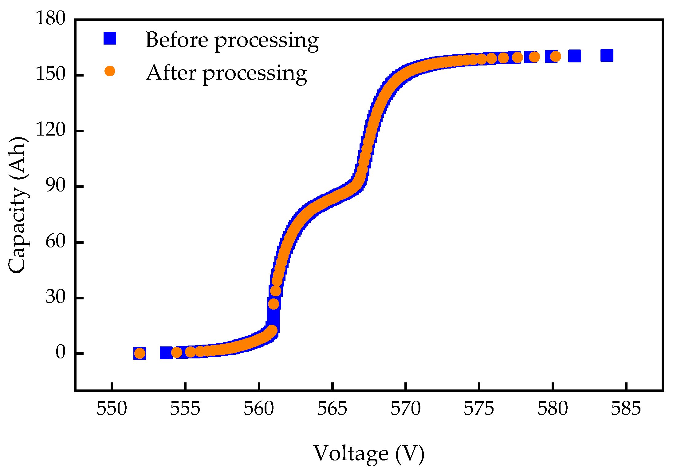
where Q t and V t denote the battery capacity and voltage at time t, respectively, whereas Q t 1 and V t 1 denote the battery capacity and voltage at time t – 1, respectively. However, the measured voltages may remain unchanged within certain successive time steps, masking the characteristics of the IC curves. To solve this issue, this paper extracts the discrete charging curve Q(V) with a sampling interval of 0.1 V, resulting in a monotonically increasing function, as illustrated in Figure 3.
The initial IC curves can be derived from the differential of the charging curve Q(V). In practice, the obtained curve is susceptible to fluctuations caused by noise, and it is challenging to identify useful features. To tackle this issue, filtering algorithms are required. Herein, two advanced filtering algorithms named the moving average (MA) filter and the Gaussian smoothing (GS) filter are compared to analyze the smooth results, and the more suitable method is chosen to smooth the IC curves.
MA is a typical linear filtering method. As shown in Equation (4), MA gives equal weight to each data point and replaces it with the average values of its neighbors for smoothing.
y ( i ) = 1 N j = 0 N 1 x ( i + j )
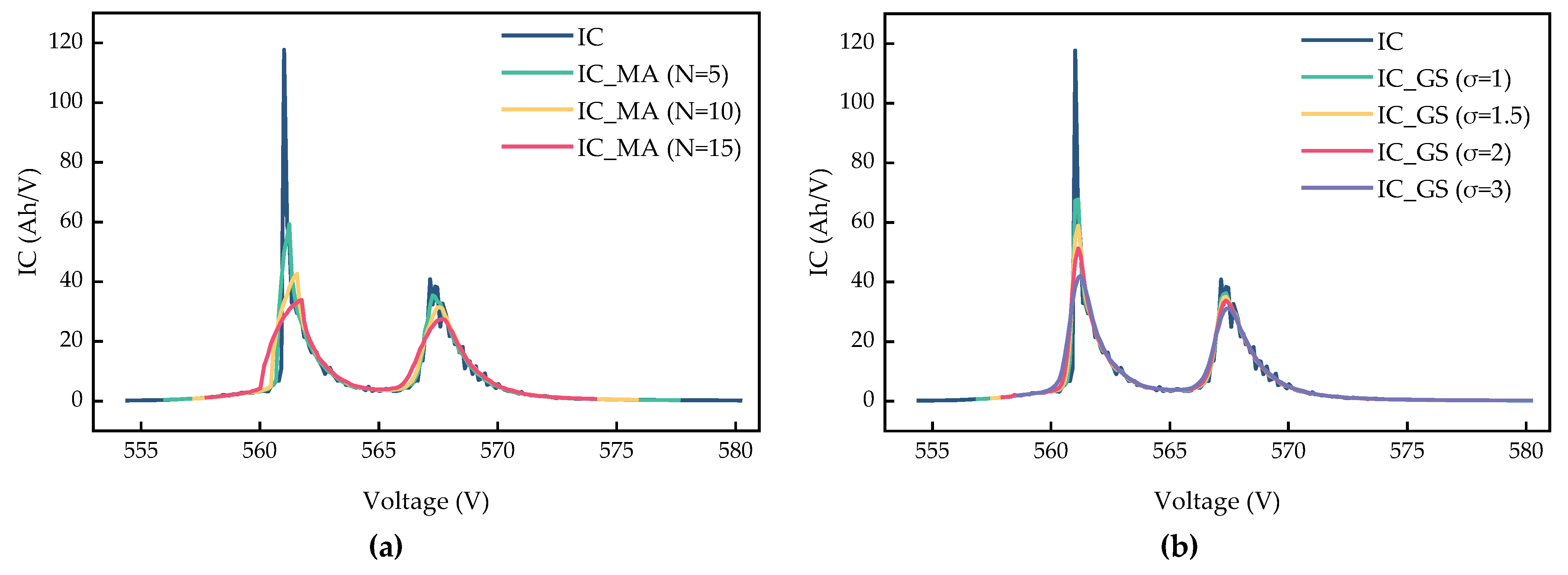
where x ( · ) is the input signal and y ( · ) is the output signal; N stands for the fixed size of the moving windows, which is closely related to the effectiveness of MA. Roughly, the larger the fixed size, the smoother the IC curves. Nevertheless, an excessively large N could potentially cause curve distortion or false interpretation of the features. Figure 4a displays an IC curve smoothed by the MA method. As the window size increases, the curve becomes smoother, but the intensity of the peaks decreases, and their positions shift towards the higher voltage range, with poor robustness. When the value of N is set to 5, the best filtering effect is achieved compared with the others.
GS eliminates fluctuations by separating low-frequency signals from high-frequency signals. The GS method has the trait of a Gaussian distribution, given in Equation (5).
G ( x ) = 1 σ 2 π exp ( ( x μ ) 2 2 σ 2 )
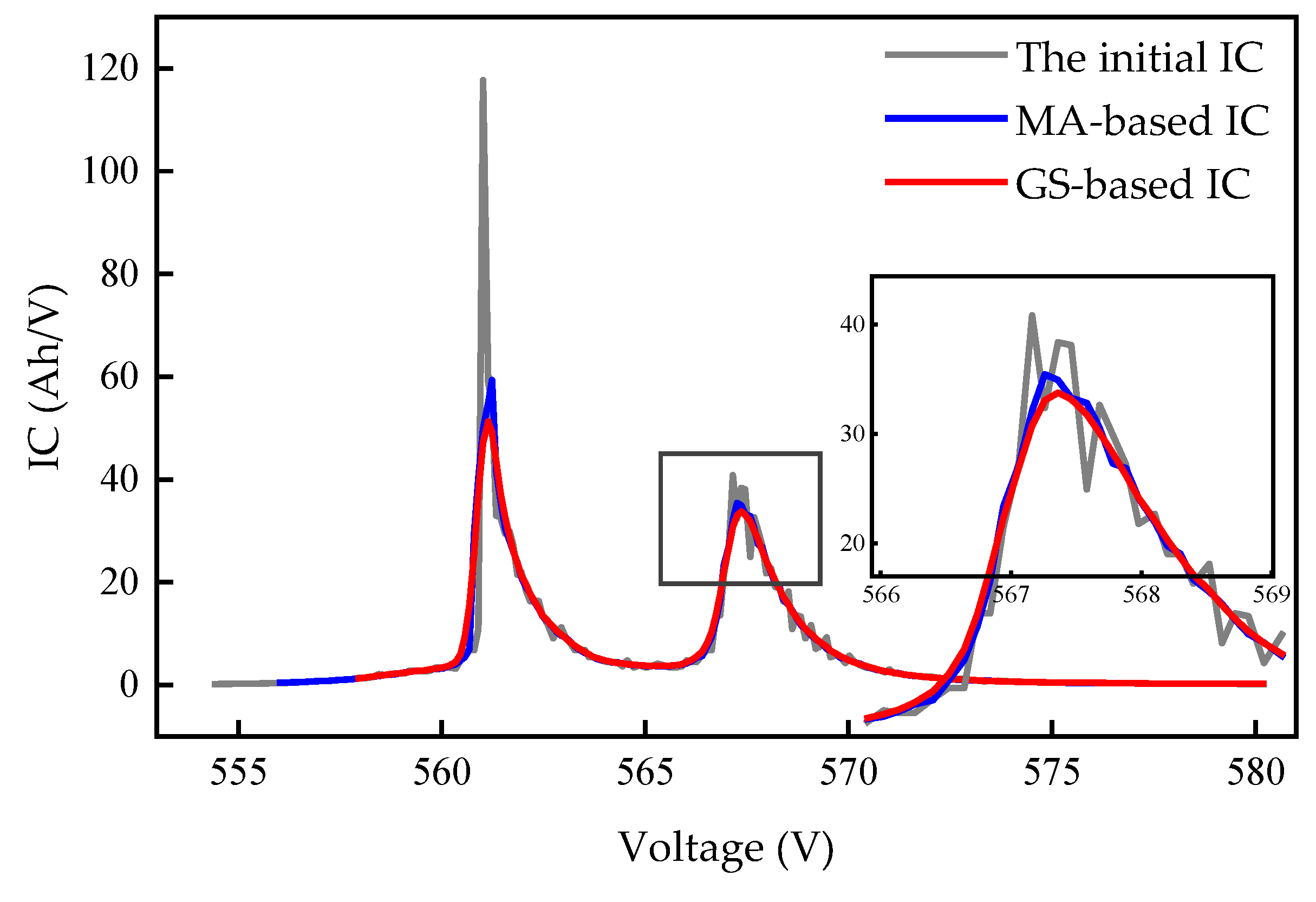
where μ and σ denote the mean value and the standard deviation, respectively. Each data point is acquired by a weighted average of neighbors in a Gaussian window, with proximity having a greater effect on the value and distance having a smaller effect. When the GS method is used to smooth the curve, μ is usually set to 0 to ensure each data point has an impact on its smoothed value. σ is positively related to the size of the Gaussian window. The larger the σ , the smoother the curve. Nevertheless, too large a σ will lead to curve distortion and false interpretation of the features. As can be observed from Figure 4b, the value of 2 gives the best filtering effect without distorting the curve. Figure 5 compares the MA method (N = 5) and GS method ( σ = 2 ); the GS method with the value of σ set to 2 is more suitable in this work.

4.2. Regional Capacity Calculation

The regional capacity is defined as the capacity obtained by Coulomb counting with constant current in a certain voltage region. Mathematically, the start point and the end point of the voltage region are used to calculate the regional capacity.
V ( t 1 ) = V p Δ V / 2
V ( t 2 ) = V p + Δ V / 2
Q r = Q ( t 2 ) Q ( t 1 )
where V p is the terminal voltage corresponding to the IC peak. V stands for the regional voltage, which is used to determine the time duration for regional capacity integration. Q r denotes the regional capacity, and Q(t) is the capacity at time t. Equations (6) and (7) are the start point and the end point of the voltage region, respectively. Equation (8) denotes the regional capacity.
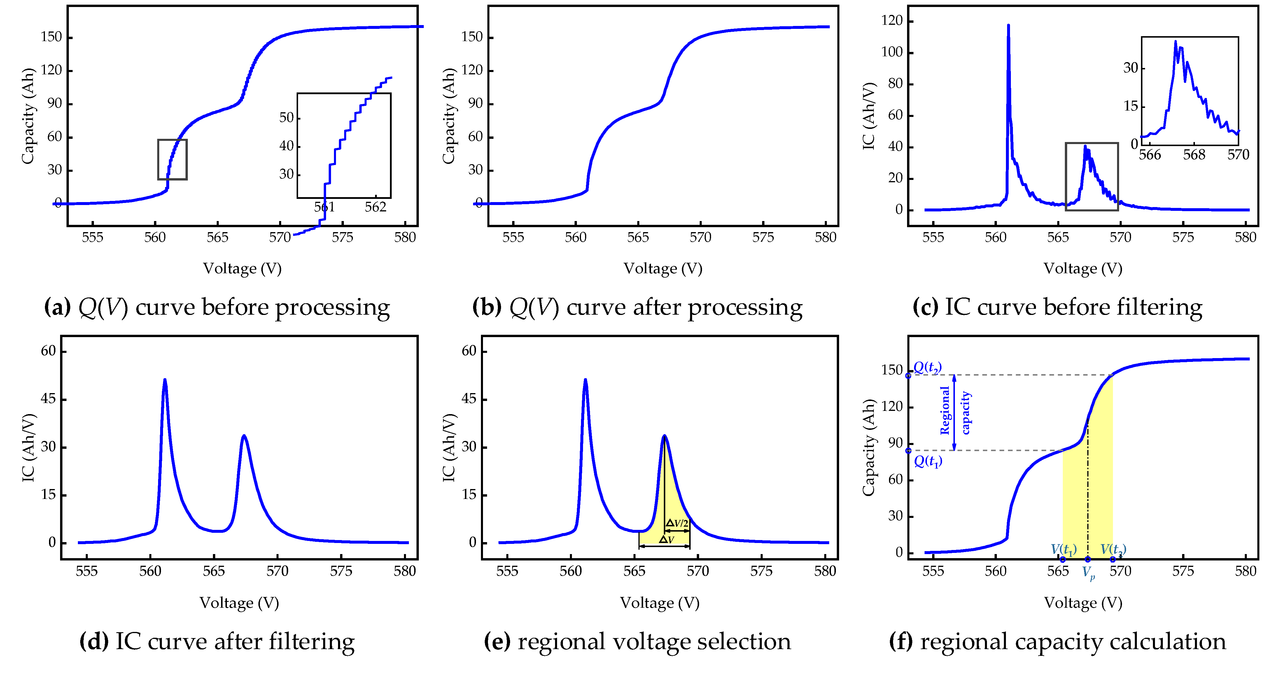
Based on the analysis presented above, the regional capacity, as in the highlighted region in Figure 6, is calculated by the following steps:
  • Step 1: Obtain the charging curve Q(V). Suitable charging segments are selected based on certain constrains. Then, the charging curve Q(V) is obtained through calculation.
  • Step 2: The monotonically increasing charging curve Q(V) is extracted to facilitate subsequent IC curve calculation.
  • Step 3: The initial IC curve is calculated through numerical derivative methods.
  • Step 4: A Gaussian smoothing filter method with a σ value of 2 is applied to smooth the calculated IC curve.
  • Step 5: The regional voltage V is determined, whose middle point corresponds to the IC peak. In this work, we choose a regional voltage of 4 V to cover the second IC peak.
  • Step 6: Calculate the regional capacity Q r .
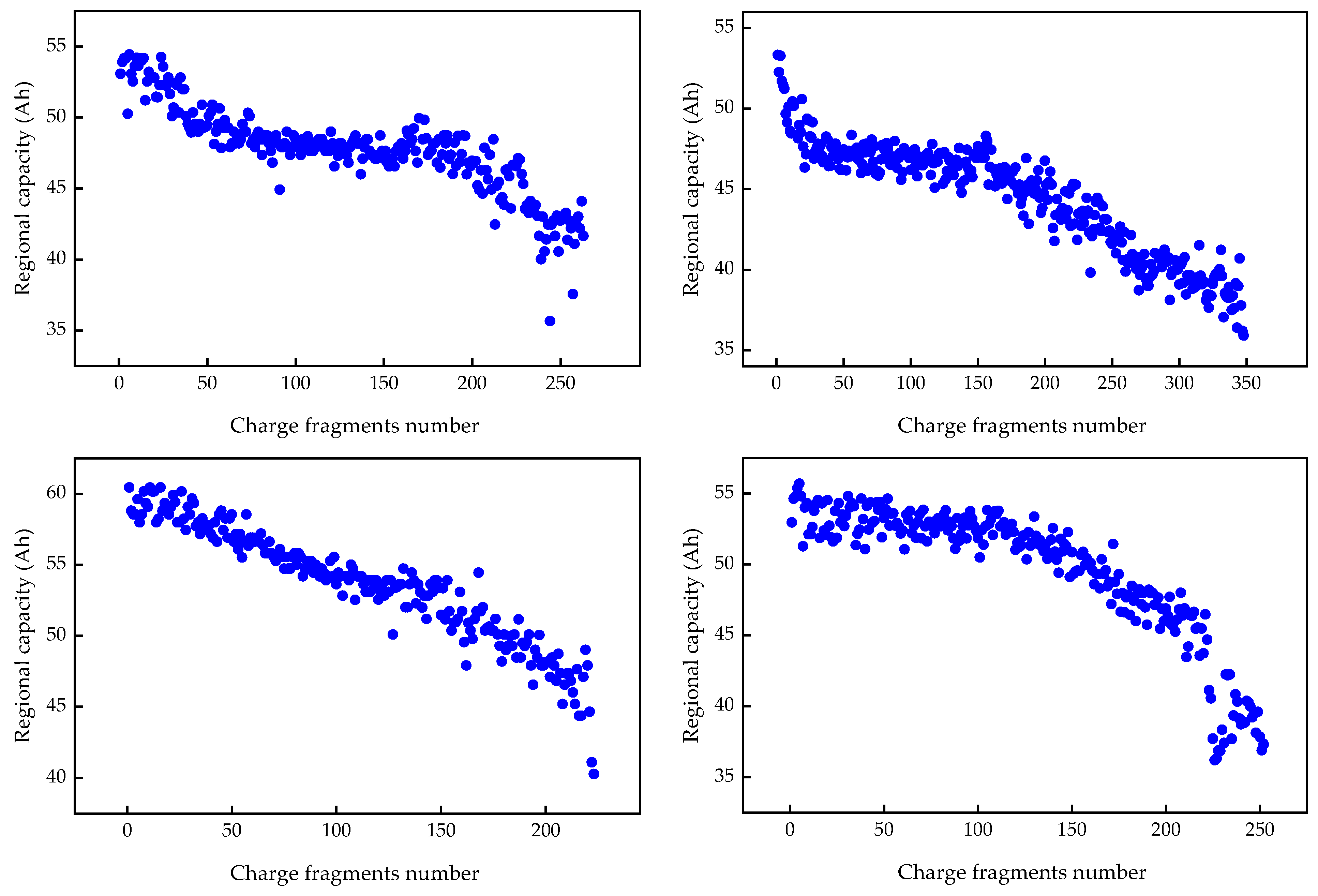
With the aforementioned steps, the regional capacity can be obtained and used for battery aging indication. The regional capacity evolution curves of four vehicles are shown in Figure 7.

4.3. Description of the LGBM Algorithm

LGBM is a boosting framework-based gradient boosting decision tree (GBDT) that combines coupled weak learners to create a stronger one [40]. By adopting a histogram-based algorithm, the leaf-wise growth strategy, gradient-based one-side sampling (GOSS), and exclusive feature bundling (EFB), excellent performance in terms of running time acceleration, memory consumption reduction, and accuracy can be achieved [41].
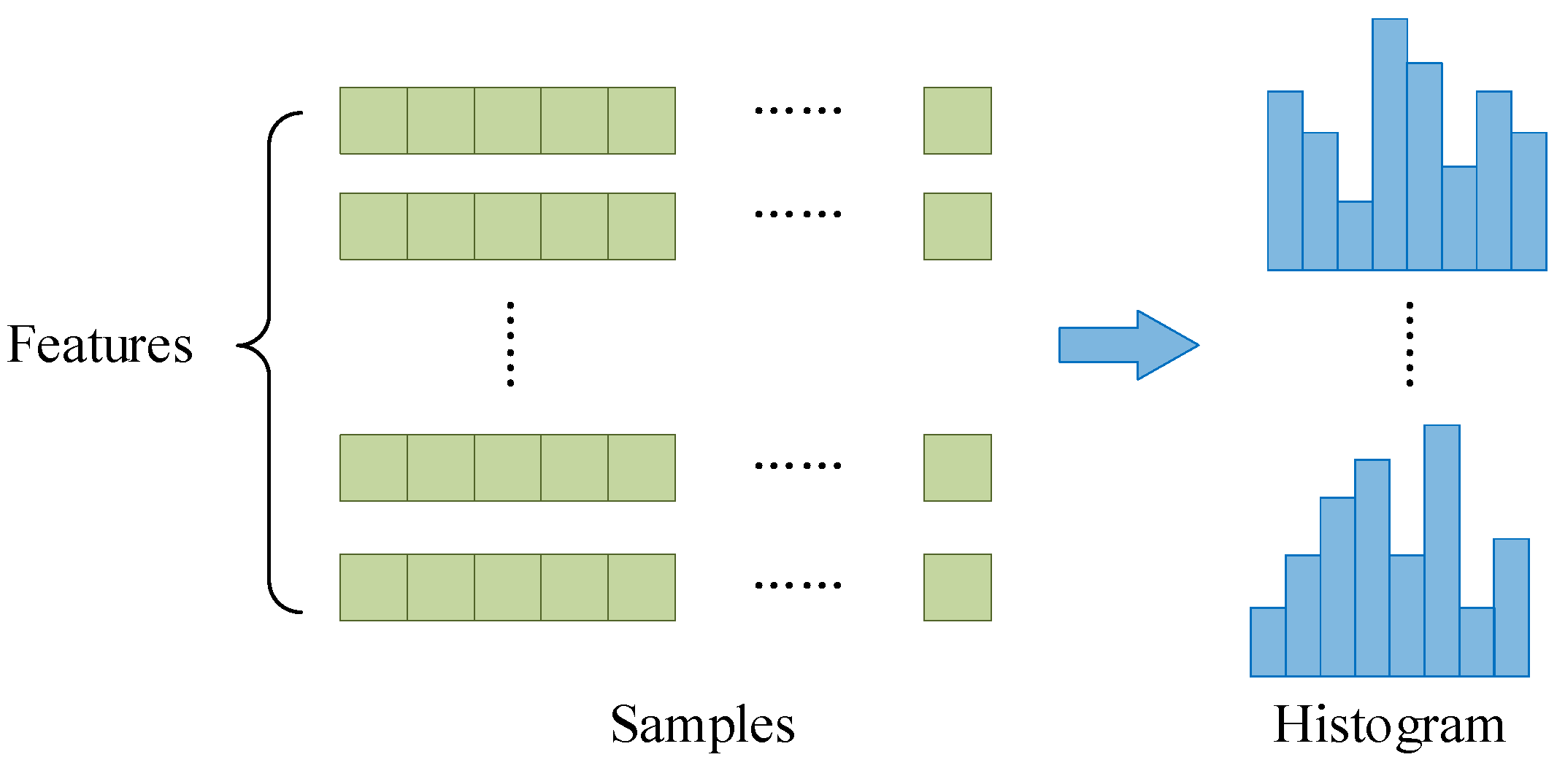
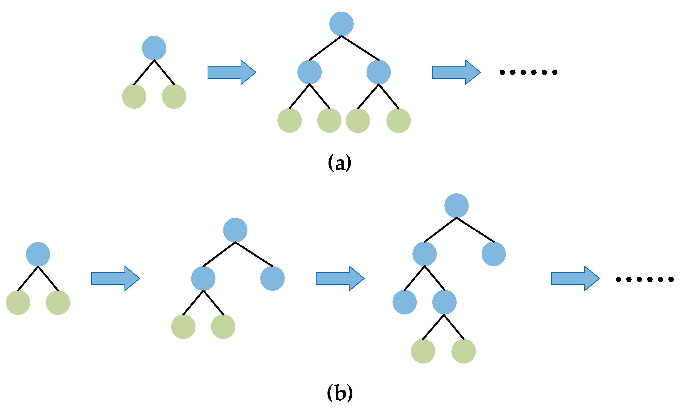
LGBM is an ensemble model of decision trees, learning the decision trees by fitting the residual errors in each iteration [42]. The most time-consuming aspect is finding the optimal split points. LGBM employs a histogram-based algorithm to find the split points. As shown in Figure 8, this algorithm buckets continuous values into discrete small bins, uses these bins to generate feature histograms, and finds split points according to the cumulative statistics of each discrete value. The histogram-based algorithm effectively reduces memory consumption and computational complexity. The method of tree growth in LGBM is the leaf-wise growth strategy with depth limitation, while the level-wise growth strategy is typically used in the conventional GBDT [43]. Figure 9 shows the differences between the level-wise growth strategy and the leaf-wise growth strategy. The leaf-wise growth strategy only enables leaves with the largest information gains to split, improving the accuracy and efficiency [44]. The objective function of LGBM is shown in Equation (9).
O b j ( t ) = L ( t ) + Ω ( t ) + c
where Ω (t) and L(t) denote the regular and loss functions, respectively, while c and t denote the extra parameter and the sampling time, respectively. The extra parameter prevents overfitting and optimizes the depth of the tree. The regular function reflects the complexity of the model. The loss function is defined in Equation (10).
L ( t ) = n = 1 n ( y i ( t ) y ^ i ( t ) ) 2
where y i is the true value, and y ^ i is the predict value.
Data with larger gradients contribute more to the information gain. In order to keep the trade-off between accuracy and efficiency, GOSS is employed in LGBM. GOSS reserves those data with large gradients and randomly samples those data with small gradients. EFB is a nearly lossless approach to reduce the number of the features because the feature space is quite sparse in real applications. Features in a sparse feature space are almost mutually exclusive, which means they hardly take nonzero values simultaneously. Therefore, the EFB algorithm can bundle many exclusive features into fewer features to avoid unnecessary computation for zero feature values, improving the training speed without hurting the accuracy.

4.4. Construction of Battery SOH Estimation Model

The construction of the battery SOH estimation model can be implemented with four steps: feature extraction, feature normalization, model training, and model evaluation. The framework of the model is shown in Figure 10.

4.4.1. Feature Extraction

A lithium-ion battery is a dynamic and time-varying electrochemical system, and its aging process is sensitive to various factors [45]. Furthermore, the sparse and discontinuous characters of the data from the real-world EVs compared to the laboratory data make the extraction of health factors difficult. Consequently, it is necessary to derive influential factors to determine the appropriate model inputs for the real-world operating vehicles. The accumulated ampere hour throughput, charging current rate, temperature, and depth of discharge (DOD) are considered the main factors that influence battery degradation in many studies [46,47,48,49]. It is necessary to select parameters that are easily available for model construction by referring to the findings of various laboratory studies. The accumulated mileage of vehicles can reflect the cumulative ampere hour throughput, which imposes a major impact on battery degradation. The average charging current can represent the charging current rate well. The average charging temperature gathered by the temperature sensors in the battery system can correspond to the ambient temperature. The start of SOC value, the end of SOC value, and the depth of charge can indicate DOD.
This study mainly focuses on charging segments after data processing in Section 2. Among these features, the accumulated mileage, start of SOC value, and end of SOC value are readily available in each charging segment. The depth of charge equals the end of SOC value minus the start of SOC value. The average current and temperature of each charging segment can be calculated by Equations (11) and (12).
I a = 1 n i = 1 n I i
T a = 1 n i = 1 n T i = 1 2 n i = 1 n ( T i max + T i min )
where I a and T a are the average current and temperature of each charging segment, respectively, n is the number of samples in a charging segment, I i and T i denote the current and average temperature at sample i, respectively, and T i max and T i min represent the highest and lowest temperature of the battery system, respectively. The average temperature of each charging segment can be approximated by the average of the highest temperature and lowest temperature of the battery system.
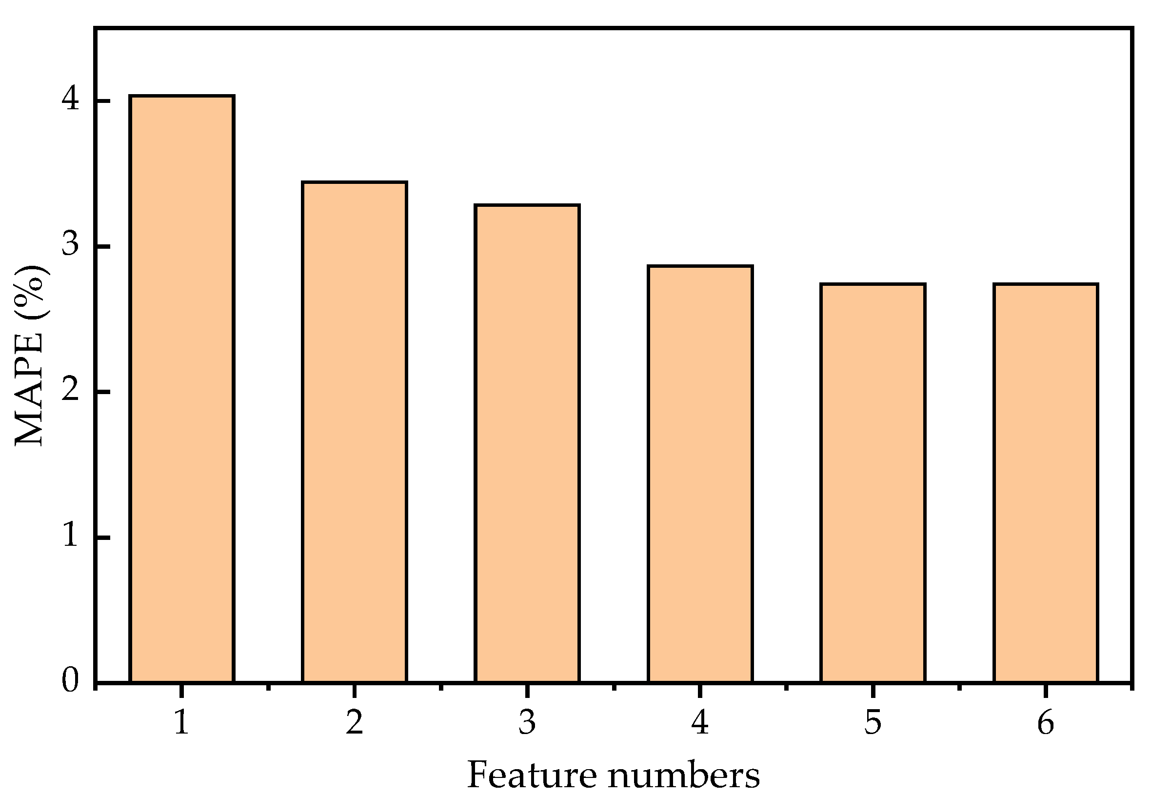
In order to maintain a balance between accuracy and computational speed, model inputs need to be condensed. The model inputs are sorted according to correlation, and features with high correlation are selected as model inputs to observe the relationship between the number of model inputs and the accuracy of the model. When the model inputs exceed five, increasing the number of model inputs has limited effect on improving the model accuracy, as can be seen from the Figure 11. Therefore, the accumulated mileage, average charging current, average charging temperature, and start and end SOC values are selected as model inputs. These model inputs can easily be extracted from the operating data, though they are sparse and discontinuous. The model outputs are the regional capacity values which are described in detail in Section 3.

4.4.2. Feature Normalization

In order to prevent the model parameters from being dominated by data with a greater or smaller distribution range, it is necessary to normalize the data after feature extraction to bring the distributions of data in all dimensions close to one another. Feature normalization can accelerate the speed of optimization and improve the accuracy.
This paper employs the linear normalization method to scale the range of features to the [0, 1] interval. The 0–1 scaling of x can be computed by Equation (13).
x ¯ i = x x min x max x min
where x denotes the initial value, xmin is the minimum value of x, xmax is the maximum value of x, and x ¯ i is the normalized value of x. After feature normalization, the convergence speed of the loss function can be accelerated, and the stability can be improved during the model training process.

4.4.3. Model Training

The datasets used for the study are randomly used for model training and test. The training and validation group contains 28 vehicles, and the other four vehicles are used as the test group to verify the effectiveness of the proposed method. The aim of model training is to minimize the errors between the model estimation values and real values.
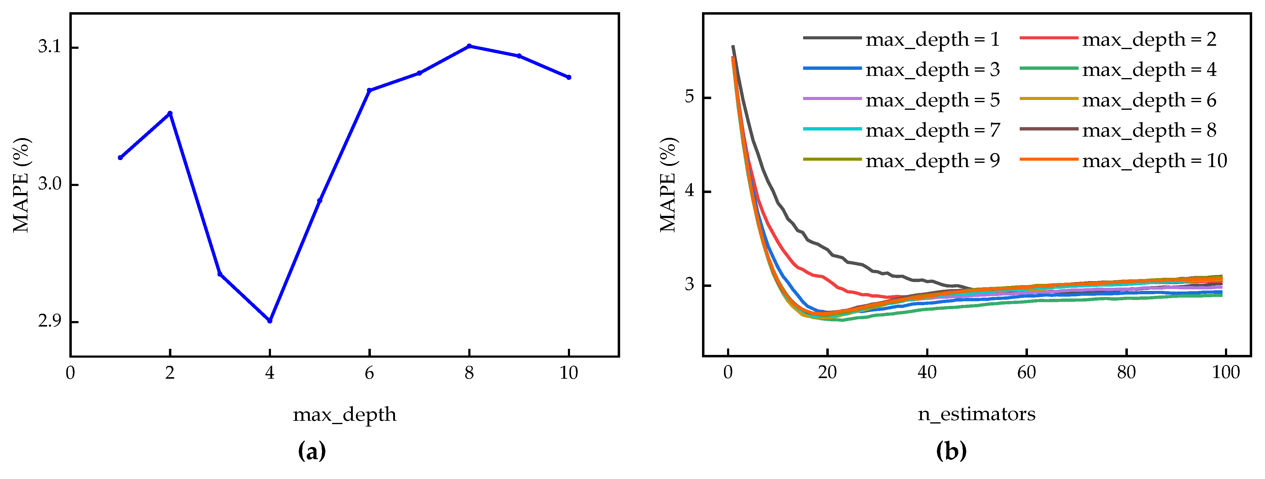
In order to improve the accuracy of the model, the hyperparameters of the LGBM model need to be optimized. It is necessary to select the parameters, which exert the dominant impact on model results, to optimize preferentially. To prevent overfitting, the max depth must be adjusted preferentially to regulate the depth of the decision tree. In addition, the number of estimators can control the number of decision trees, which is closely related to the model accuracy. Herein, the hyperparameters selected for optimization include the max depth and the number of estimators. The ranges of both hyperparameters are set to 1–10 and 1–100. Figure 12 illustrates the variations of MAPE with the changes of the hyperparameters. In this paper, the max depth and the number of estimators are 4 and 23, respectively. After hyperparameter optimization, the best combination of hyperparameters is selected to establish the SOH estimation model.

4.4.4. Model Evaluation

The final model is generated by inputting the optimal LGBM hyperparameters, and it is then applied to the test datasets to validate the effectiveness of the proposed method. The absolute error (e), relative error (er), mean absolute percentage error (MAPE), and root mean square error (RMSE) are chosen to evaluate the performance of the SOH estimation models.
e = y k y k
e r = y k y k y k × 100 %
M A P E = 1 n k = 1 n k y k y y k × 100 %
R M S E = 1 n k = 1 n ( y k y k ) 2
where y k is the true regional capacity, y ^ k is the predicted value, and n is the number of samples. Equations (14)–(17) are the absolute error, relative error, MAPE, and RMSE, respectively.

5. Results and Discussions

5.1. Verification in Real-World EVs

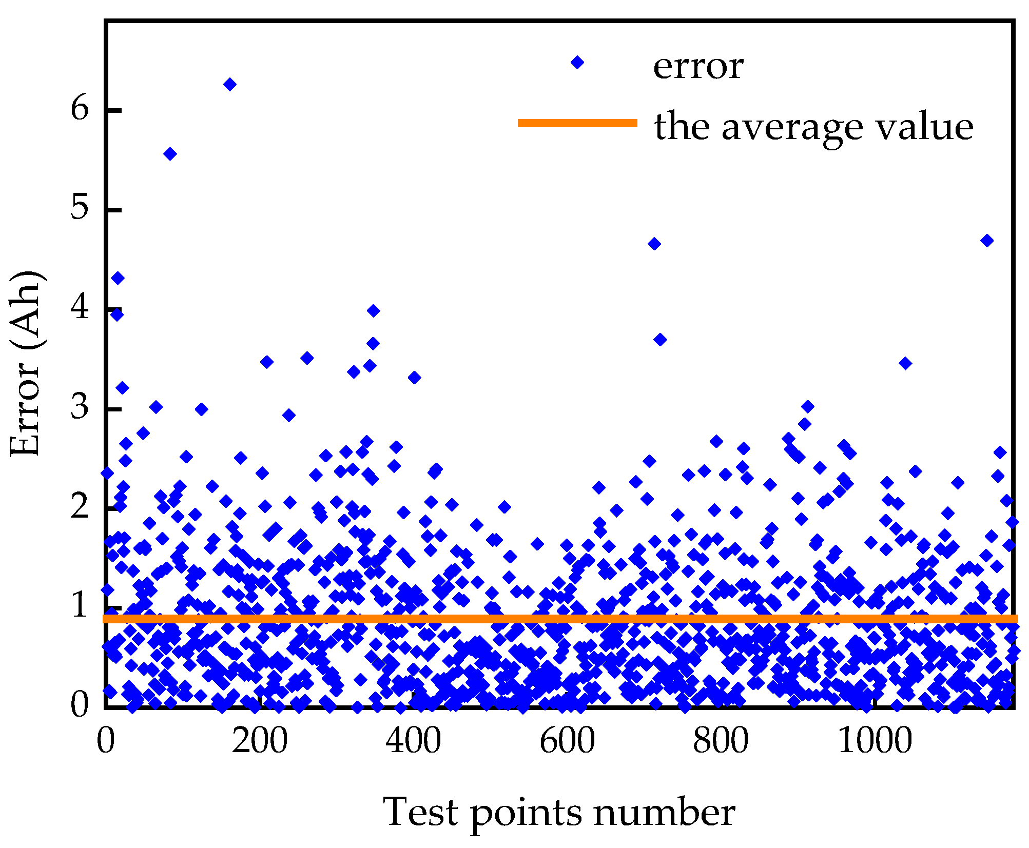
This section shows the effectiveness of the SOH estimation model based on the test datasets. Figure 13 illustrates the absolute error for the test datasets. We can see that the LGBM model can accurately estimate the regional capacity, and the average absolute error is only 0.89 Ah. According to Equations (16) and (17), the MAPE and RMSE are 2.049% and 1.153%, respectively.
As a brief conclusion, the proposed method is effective in online real-time battery SOH estimation for the following reasons. Firstly, the model inputs include the accumulated mileage, average charging current, average charging temperature, and start and end SOC values. Most of these can be directly acquired from the operating data, whereas the rest can be obtained through simple mathematical calculations. Secondly, the runtime of online estimation method based on four test vehicles using a personal computer is only 0.069 s. The runtime can be considered negligible in relation to the time taken to gather the sensor data of the EVs. Thirdly, the estimation only occupies 213.62 MB of memory, which makes online estimation possible.

5.2. Comparative Analysis of Different Algorithms

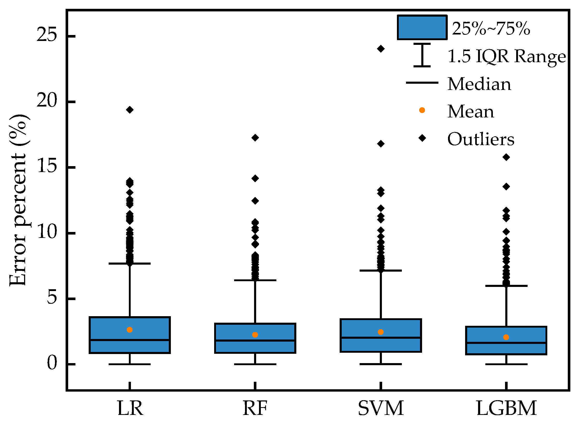
To demonstrate the superiority of the proposed method, a comparison study is performed to compare the proposed method with the linear regression (LR), random forest (RF), and SVM-based SOH estimation algorithms. The distribution of the estimations’ relative errors are plotted in Figure 14 for a more intuitive view. The estimation results from the proposed method have the highest accuracy with the smallest maximum error and a generally smaller error rate, indicating its superior ability compared with LR, RF, and SVM.
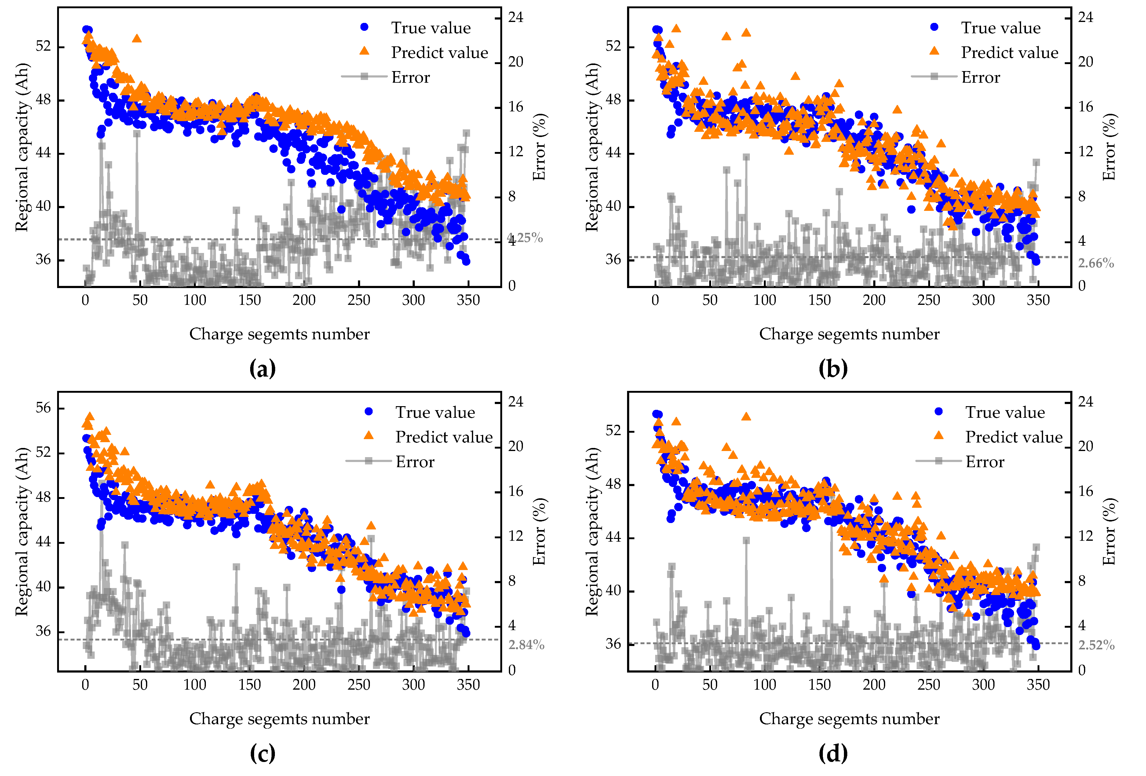
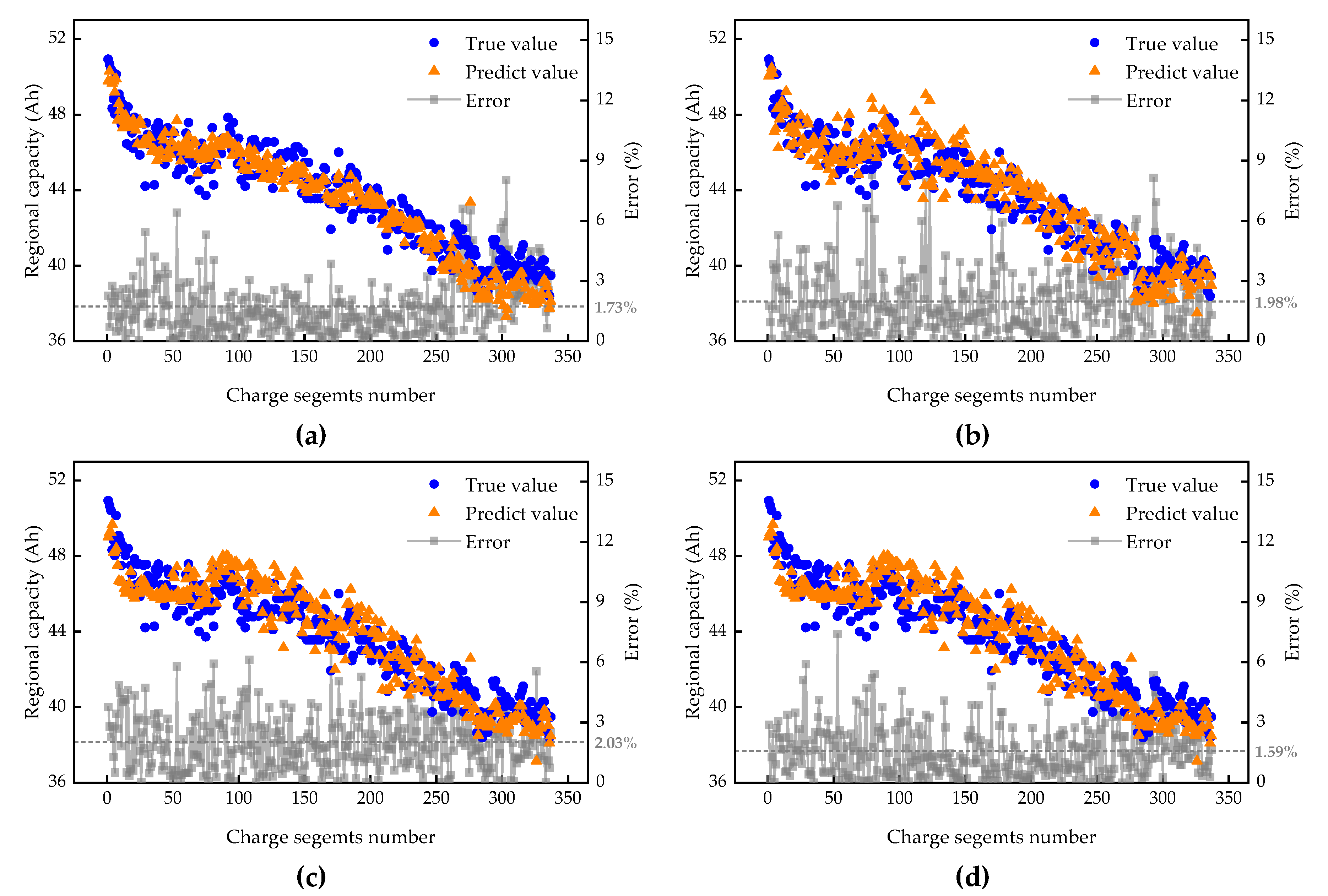
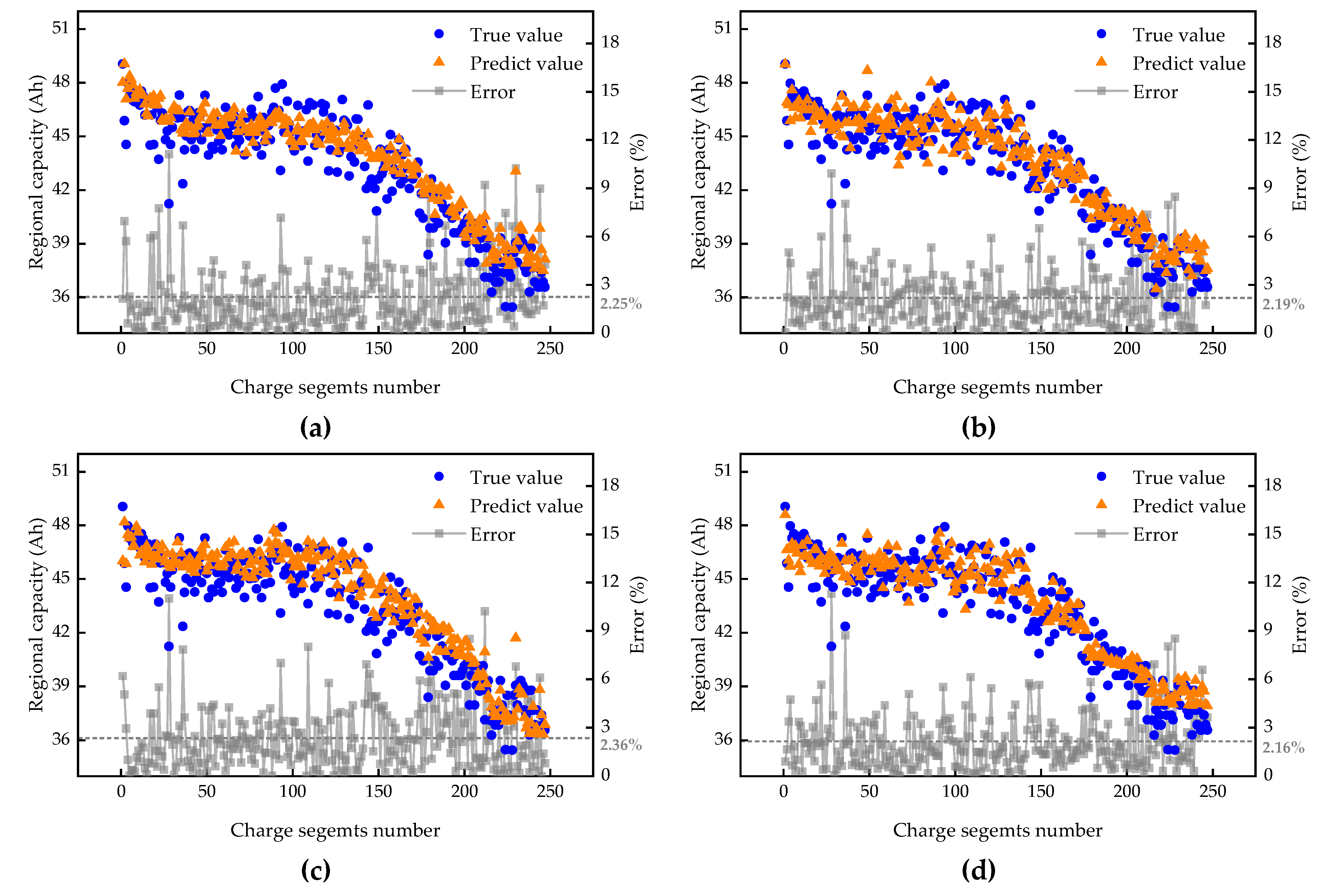
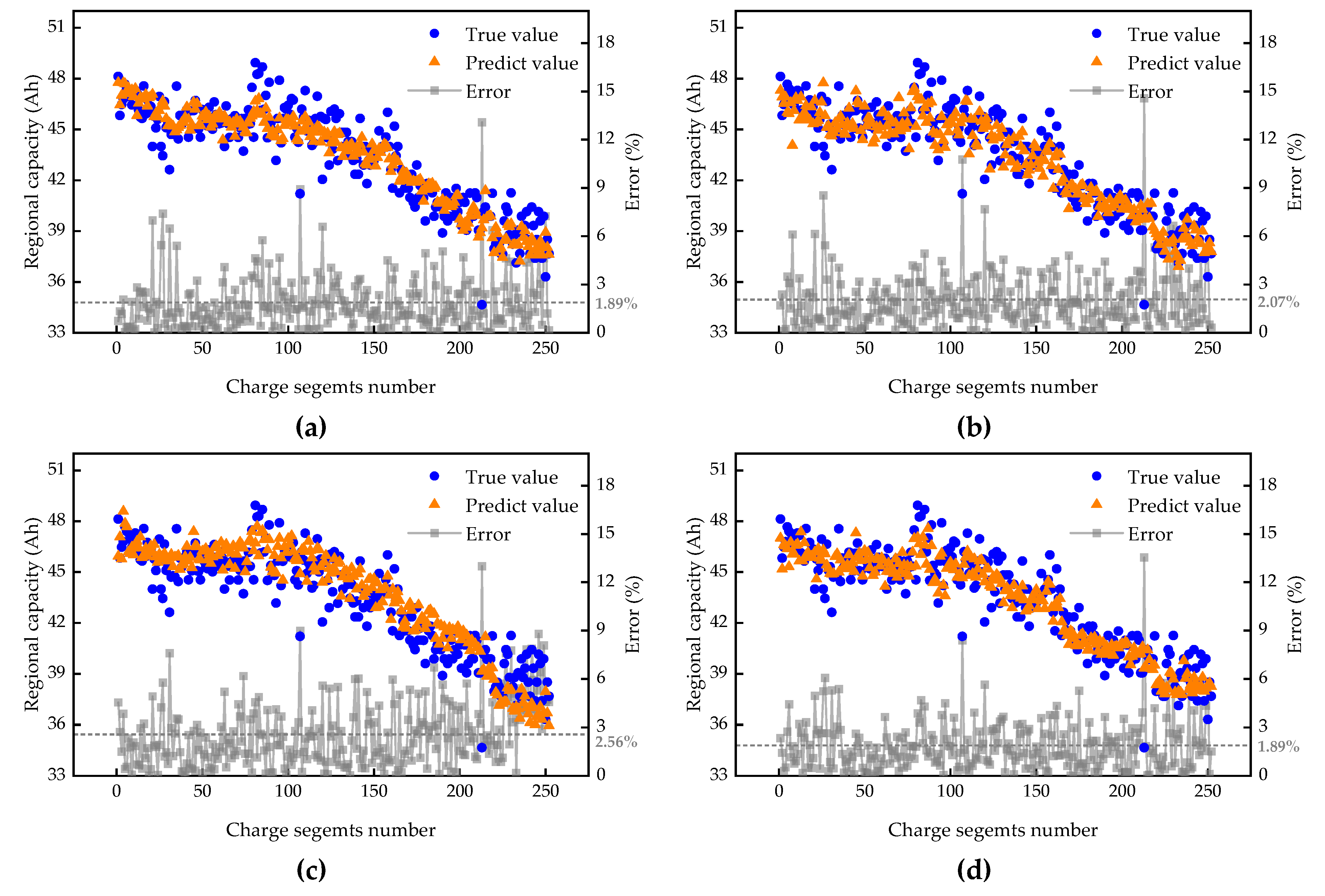
The test datasets contain four vehicles which are completely different from the ones used for model training. In order to better observe the battery SOH estimation effect for the four different test vehicles, Figure 15, Figure 16, Figure 17 and Figure 18 show the SOH estimation results of different vehicles based on different data-driven algorithms, and the statistical errors are summarized in Table 4.
Figure 15 illustrates the capacity estimation results of test vehicle 1 based on different data-driven algorithms. The LGBM has the best accuracy, and its MAPE and RMSE are only 2.520% and 1.403% in the test process, respectively, while LR has the worst accuracy, and its MAPE and RMSE are 4.254% and 2.208% in the test process, respectively. Figure 16 illustrates the capacity estimation results of test vehicle 2 based on different data-driven algorithms. The LGBM has the best accuracy, and its MAPE and RMSE are only 1.598% and 0.893% in the test process, respectively, while SVM has the worst accuracy, and its MAPE and RMSE are 2.034% and 1.078% in the test process, respectively. Figure 17 illustrates the capacity estimation results of test vehicle 3 based on different data-driven algorithms. The LGBM has the best accuracy, and its MAPE and RMSE are only 2.158% and 1.164% in the test process, respectively, while SVM has the worst accuracy, and its MAPE and RMSE are 2.363% and 1.288% in the test process, respectively. Figure 18 illustrates the capacity estimation results of test vehicle 4 based on different data-driven algorithms. The LGBM has the best accuracy, and its MAPE and RMSE are only 1.898% and 1.065% in the test process, respectively, while SVM has the worst accuracy, and its MAPE and RMSE are 2.564% and 1.362% in the test process, respectively.
The results demonstrate the superiority of the LGBM model. The LGBM model has higher estimation accuracy compared to other methods.

5.3. Sensitivity Analysis

The proposed LGBM model is further implemented using data with noise for sensitivity analysis. White noise is added to all the model inputs of the test datasets before they are forwarded to the model. The maximum noise rates are set to 1%, 2%, 3%, and 5%. As can be seen in Table 5, the range of MAPEs under different noise intensities is from 2.354% to 2.881%, and the range of RMSEs is from 1.401% to 1.663%. The results validate the high accuracy and good robustness of the proposed method against noise corruption.

6. Conclusions

This paper provides a battery SOH estimation method for battery systems in real-world EVs based on the LGBM algorithm. The regional capacity is utilized as the benchmark of SOH estimation and is derived by the ICA method together with a GS filter. The accumulated mileage, average charging current, average charging temperature, and start and end SOC values are chosen as the model inputs. The datasets used for the study are collected from real-world electric city transit buses. Datasets from 28 vehicles are employed for model training and validation, while datasets acquired from four other vehicles are employed to verify the performance of the model. The effectiveness, low complexity, superiority, and robustness of the proposed method are verified based on the test datasets. The model achieves satisfactory accuracy, with an average absolute error of only 0.89 Ah. The MAPE and RMSE of the test vehicles are 2.049% and 1.153%, respectively. Furthermore, the model’s robustness against noise corruption is also verified. Thanks to the lower computational complexity of the feature extraction and the rapidity and accuracy of the model estimation, the proposed method is a very useful tool in battery SOH estimation for large-scale operating EVs and has great potential to be integrated into an embedded BMS.

Author Contributions

Conceptualization, Z.Z. and N.L.; methodology, S.W.; software, S.W.; validation, S.W.; formal analysis, Z.Z.; investigation, N.L.; resources, P.L. and Z.W.; data curation, P.L. and Z.W.; writing—original draft preparation, S.W.; writing—review and editing, N.L.; visualization, Z.Z.; supervision, N.L. and P.L.; project administration, Z.W.; funding acquisition, Z.W. All authors have read and agreed to the published version of the manuscript.

Funding

This work was supported by the National Key Research and Development Program of China (Grant No. 2019YFE0104700), the National Science Foundation of China (Grant No. 52172398) and Shandong Provincial Science Foundation (Grant No. ZR2021ME065).

Institutional Review Board Statement

Not applicable.

Informed Consent Statement

Not applicable.

Data Availability Statement

Data sharing is not applicable.

Conflicts of Interest

The authors declare no conflict of interest.

Nomenclatures

AbbreviationDescription
SOHState of health
EVsElectric vehicles
LGBMLight gradient boosting machine
ICAIncremental capacity analysis
GSGaussian smoothing
BMSBattery management system
EISElectrochemical impedance spectroscopy
EMsElectrochemical models
ECMsEquivalent circuit models
LSLeast squares
KFKalman filter
PFParticle filter
SVMSupport vector machine
GPRGaussian process regression
ANNArtificial neural network
NDANEVNational Big Data Alliance of New Energy Vehicles
MAMoving average
GBDTGradient boosting decision tree
GOSSGradient-based one-side sampling
EFBExclusive feature bundling
DODDepth of discharge
MAPEMean absolute percentage error
RMSERoot mean square error
LRLinear regression
RFRandom forest

References

  1. Ng, M.-F.; Zhao, J.; Yan, Q.; Conduit, G.J.; Seh, Z.W. Predicting the state of charge and health of batteries using data-driven machine learning. Nat. Mach. Intell. 2020, 2, 161–170. [Google Scholar] [CrossRef] [Green Version]
  2. Mitova, S.; Henao, A.; Kahsar, R.; Farmer, C.J.Q. Smart Charging for Electric Ride-Hailing Vehicles using Renewables: A San Francisco Case Study. Int. J. Sustain. Energy Environ. Res. 2022, 11, 67–85. [Google Scholar] [CrossRef]
  3. Dwijendra, N.K.A.; Sharma, S.; Asary, A.R.; Majdi, A.; Muda, I.; Mutlak, D.A.; Parra, R.M.R.; Hammid, A.T. Economic performance of a hybrid renewable energy system with optimal design of resources. Environ. Clim. Technol. 2022, 26, 441–453. [Google Scholar] [CrossRef]
  4. Harper, G.; Sommerville, R.; Kendrick, E.; Driscoll, L.; Slater, P.; Stolkin, R.; Walton, A.; Christensen, P.; Heidrich, O.; Lambert, S.; et al. Recycling lithium-ion batteries from electric vehicles. Nature 2019, 575, 75–86. [Google Scholar] [CrossRef] [Green Version]
  5. Goli, A.; Golmohammadi, A.-M.; Verdegay, J.-L. Two-echelon electric vehicle routing problem with a developed moth-flame meta-heuristic algorithm. Oper. Manag. Res. 2022, 15, 891–912. [Google Scholar] [CrossRef]
  6. Feng, F.; Teng, S.; Liu, K.; Xie, J.; Xie, Y.; Liu, B.; Li, K. Co-estimation of lithium-ion battery state of charge and state of temperature based on a hybrid electrochemical-thermal-neural-network model. J. Power Sources 2020, 455, 227935. [Google Scholar] [CrossRef]
  7. Zhou, L.; Zhao, Y.; Li, D.; Wang, Z. State-of-Health Estimation for LiFePO4 Battery System on Real-World Electric Vehicles Considering Aging Stage. IEEE Trans. Transp. Electrif. 2022, 8, 1724–1733. [Google Scholar] [CrossRef]
  8. Li, G.; Chen, H.; Zhang, B.; Guo, H.; Chen, S.; Chang, X.; Wu, X.; Zheng, J.; Li, X. Interfacial covalent bonding enables transition metal phosphide superior lithium storage performance. Appl. Surf. Sci. 2022, 582, 152404. [Google Scholar] [CrossRef]
  9. Roman, D.; Saxena, S.; Robu, V.; Pecht, M.; Flynn, D. Machine learning pipeline for battery state-of-health estimation. Nat. Mach. Intell. 2021, 3, 447–456. [Google Scholar] [CrossRef]
  10. Li, Y.; Liu, K.; Foley, A.M.; Zülke, A.; Berecibar, M.; Nanini-Maury, E.; Van Mierlo, J.; Hoster, H.E. Data-driven health estimation and lifetime prediction of lithium-ion batteries: A review. Renew. Sust. Energy Rev. 2019, 113, 109254. [Google Scholar] [CrossRef]
  11. Wang, Q.; Wang, Z.; Zhang, L.; Liu, P.; Zhang, Z. A novel consistency evaluation method for series-connected battery systems based on real-world operation data. IEEE Trans. Transp. Electrif. 2020, 7, 437–451. [Google Scholar] [CrossRef]
  12. She, C.; Li, Y.; Zou, C.; Wik, T.; Wang, Z.; Sun, F. Offline and Online Blended Machine Learning for Lithium-Ion Battery Health State Estimation. IEEE Trans. Transp. Electrif. 2021, 8, 1604–1618. [Google Scholar] [CrossRef]
  13. Li, W.; Sengupta, N.; Dechent, P.; Howey, D.; Annaswamy, A.; Sauer, D.U. Online capacity estimation of lithium-ion batteries with deep long short-term memory networks. J. Power Sources 2021, 482. [Google Scholar] [CrossRef]
  14. Zhang, S.; Guo, X.; Dou, X.; Zhang, X. A rapid online calculation method for state of health of lithium-ion battery based on coulomb counting method and differential voltage analysis. J. Power Sources 2020, 479, 228740. [Google Scholar] [CrossRef]
  15. Lyu, Z.; Gao, R.; Li, X. A partial charging curve-based data-fusion-model method for capacity estimation of Li-Ion battery. J. Power Sources 2021, 483, 229131. [Google Scholar] [CrossRef]
  16. Fu, Y.; Xu, J.; Shi, M.; Mei, X. A Fast Impedance Calculation-Based Battery State-of-Health Estimation Method. IEEE Trans. Ind. Electron. 2022, 69, 7019–7028. [Google Scholar] [CrossRef]
  17. Jiang, B.; Zhu, J.; Wang, X.; Wei, X.; Shang, W.; Dai, H. A comparative study of different features extracted from electrochemical impedance spectroscopy in state of health estimation for lithium-ion batteries. Appl. Energy 2022, 322, 119502. [Google Scholar] [CrossRef]
  18. Gao, Y.; Liu, K.; Zhu, C.; Zhang, X.; Zhang, D. Co-Estimation of State-of-Charge and State-of- Health for Lithium-Ion Batteries Using an Enhanced Electrochemical Model. IEEE Trans. Ind. Electronif. 2022, 69, 2684–2696. [Google Scholar] [CrossRef]
  19. Han, X.; Ouyang, M.; Lu, L.; Li, J. Simplification of physics-based electrochemical model for lithium ion battery on electric vehicle. Part I: Diffusion simplification and single particle model. J. Power Sources 2015, 278, 802–813. [Google Scholar] [CrossRef]
  20. Han, X.; Ouyang, M.; Lu, L.; Li, J. Simplification of physics-based electrochemical model for lithium ion battery on electric vehicle. Part II: Pseudo-two-dimensional model simplification and state of charge estimation. J. Power Sources 2015, 278, 814–825. [Google Scholar] [CrossRef]
  21. Yan, W.; Zhang, B.; Zhao, G.; Tang, S.; Niu, G.; Wang, X. A battery management system with a lebesgue-sampling-based extended kalman filter. IEEE T. Ind. Electron. 2019, 66, 3227–3236. [Google Scholar] [CrossRef]
  22. Yang, J.; Cai, Y.; Mi, C.C. State-of-Health Estimation for Lithium-Ion Batteries Based on Decoupled Dynamic Characteristic of Constant-Voltage Charging Current. IEEE Trans. Transp. Electrif. 2022, 8, 2070–2079. [Google Scholar] [CrossRef]
  23. Liang, K.; Zhang, Z.; Liu, P.; Wang, Z.; Jiang, S. Data-Driven Ohmic Resistance Estimation of Battery Packs for Electric Vehicles. Energies 2019, 12, 4772. [Google Scholar] [CrossRef] [Green Version]
  24. Wang, S.; Fernandez, C.; Yu, C.; Fan, Y.; Cao, W.; Stroe, D.-I. A novel charged state prediction method of the lithium ion battery packs based on the composite equivalent modeling and improved splice Kalman filtering algorithm. J. Power Sources 2020, 471, 228450. [Google Scholar] [CrossRef]
  25. Lai, X.; Wang, S.; Ma, S.; Xie, J.; Zheng, Y. Parameter sensitivity analysis and simplification of equivalent circuit model for the state of charge of lithium-ion batteries. Electrochim. Acta 2020, 330, 135239. [Google Scholar] [CrossRef]
  26. Tian, J.; Xiong, R.; Shen, W.; Lu, J.; Sun, F. Flexible battery state of health and state of charge estimation using partial charging data and deep learning. Energy Storage Mater. 2022, 51, 372–381. [Google Scholar] [CrossRef]
  27. El-kenawy, E.-S.M.; Abutarboush, H.F.; Mohamed, A.W.; Ibrahim, A. Advance artificial intelligence technique for designing double t-shaped monopole antenna. Comput. Mater. Con. 2021, 69, 2983–2995. [Google Scholar] [CrossRef]
  28. Wei, Z.; Ruan, H.; Li, Y.; Li, J.; Zhang, C.; He, H. Multistage State of Health Estimation of Lithium-Ion Battery With High Tolerance to Heavily Partial Charging. IEEE Trans. Power Electr. 2022, 37, 7432–7442. [Google Scholar] [CrossRef]
  29. Weng, C.; Cui, Y.; Sun, J.; Peng, H. On-board state of health monitoring of lithium-ion batteries using incremental capacity analysis with support vector regression. J. Power Sources 2013, 235, 36–44. [Google Scholar] [CrossRef]
  30. Li, X.; Yuan, C.; Li, X.; Wang, Z. State of health estimation for Li-Ion battery using incremental capacity analysis and Gaussian process regression. Energy 2020, 190, 116467. [Google Scholar] [CrossRef]
  31. Tian, J.; Xiong, R.; Shen, W.; Lu, J.; Yang, X.-G. Deep neural network battery charging curve prediction using 30 points collected in 10 min. Joule 2021, 5, 1521–1534. [Google Scholar] [CrossRef]
  32. Hsu, C.-W.; Xiong, R.; Chen, N.-Y.; Li, J.; Tsou, N.-T. Deep neural network battery life and voltage prediction by using data of one cycle only. Appl. Energy 2022, 306, 118134. [Google Scholar] [CrossRef]
  33. Sun, T.; Xu, B.; Cui, Y.; Feng, X.; Han, X.; Zheng, Y. A sequential capacity estimation for the lithium-ion batteries combining incremental capacity curve and discrete Arrhenius fading model. J. Power Sources 2021, 484, 229248. [Google Scholar] [CrossRef]
  34. Li, Y.; Abdel-Monem, M.; Gopalakrishnan, R.; Berecibar, M.; Nanini-Maury, E.; Omar, N.; van den Bossche, P.; Van Mierlo, J. A quick on-line state of health estimation method for Li-ion battery with incremental capacity curves processed by Gaussian filter. J. Power Sources 2018, 373, 40–53. [Google Scholar] [CrossRef]
  35. Zhang, Y.; Liu, Y.; Wang, J.; Zhang, T. State-of-health estimation for lithium-ion batteries by combining model-based incremental capacity analysis with support vector regression. Energy 2022, 239, 121986. [Google Scholar] [CrossRef]
  36. Ospina Agudelo, B.; Zamboni, W.; Monmasson, E. Application domain extension of incremental capacity-based battery SoH indicators. Energy 2021, 234, 121224. [Google Scholar] [CrossRef]
  37. Bian, X.; Wei, Z.; He, J.; Yan, F.; Liu, L. A Novel Model-Based Voltage Construction Method for Robust State-of-Health Estimation of Lithium-Ion Batteries. IEEE Trans. Ind. Electron. 2021, 68, 12173–12184. [Google Scholar] [CrossRef]
  38. Tang, X.; Zou, C.; Yao, K.; Chen, G.; Liu, B.; He, Z.; Gao, F. A fast estimation algorithm for lithium-ion battery state of health. J. Power Sources 2018, 396, 453–458. [Google Scholar] [CrossRef]
  39. Liu, P.; Wu, Y.; She, C.; Wang, Z.; Zhang, Z. Comparative Study of Incremental Capacity Curve Determination Methods for Lithium-Ion Batteries Considering the Real-World Situation. IEEE Trans. Power Electron. 2022, 37, 12563–12576. [Google Scholar] [CrossRef]
  40. Chakraborty, D.; Elhegazy, H.; Elzarka, H.; Gutierrez, L. A novel construction cost prediction model using hybrid natural and light gradient boosting. Adv. Eng. Inform. 2020, 46, 101201. [Google Scholar] [CrossRef]
  41. Ke, G.; Meng, Q.; Finley, T.; Wang, T.; Chen, W.; Ma, W.; Ye, Q.; Liu, T.-Y. Lightgbm: A highly efficient gradient boosting decision tree. Adv. Neural Inf. Process. Syst. 2017, 30, 1–9. [Google Scholar]
  42. Chen, C.; Zhang, Q.; Ma, Q.; Yu, B. LightGBM-PPI: Predicting protein-protein interactions through LightGBM with multi-information fusion. Chemometr. Intell. Lab. 2019, 191, 54–64. [Google Scholar] [CrossRef]
  43. Zhou, B.; Xu, J.; Han, F.; Yan, F.; Peng, S.; Li, Q.; Jiao, F. Pressure of different gases injected into large-scale coal matrix: Analysis of time–space dependence and prediction using light gradient boosting machine. Fuel 2020, 279, 118448. [Google Scholar] [CrossRef]
  44. Massaoudi, M.; Refaat, S.S.; Chihi, I.; Trabelsi, M.; Oueslati, F.S.; Abu-Rub, H. A novel stacked generalization ensemble-based hybrid LGBM-XGB-MLP model for Short-Term Load Forecasting. Energy 2021, 214, 118874. [Google Scholar] [CrossRef]
  45. Hu, X.; Xu, L.; Lin, X.; Pecht, M. Battery Lifetime Prognostics. Joule 2020, 4, 310–346. [Google Scholar] [CrossRef]
  46. Birkl, C.R.; Roberts, M.R.; McTurk, E.; Bruce, P.G.; Howey, D.A. Degradation diagnostics for lithium ion cells. J. Power Sources 2017, 341, 373–386. [Google Scholar] [CrossRef]
  47. Kabir, M.M.; Demirocak, D.E. Degradation mechanisms in Li-ion batteries: A state-of-the-art review. Int. J. Energy Res. 2017, 41, 1963–1986. [Google Scholar] [CrossRef]
  48. Han, X.; Lu, L.; Zheng, Y.; Feng, X.; Li, Z.; Li, J.; Ouyang, M. A review on the key issues of the lithium ion battery degradation among the whole life cycle. eTransportation 2019, 1, 100005. [Google Scholar] [CrossRef]
  49. Woody, M.; Arbabzadeh, M.; Lewis, G.M.; Keoleian, G.A.; Stefanopoulou, A. Strategies to limit degradation and maximize Li-ion battery service lifetime—Critical review and guidance for stakeholders. J. Energy Storage 2020, 28, 101231. [Google Scholar] [CrossRef]
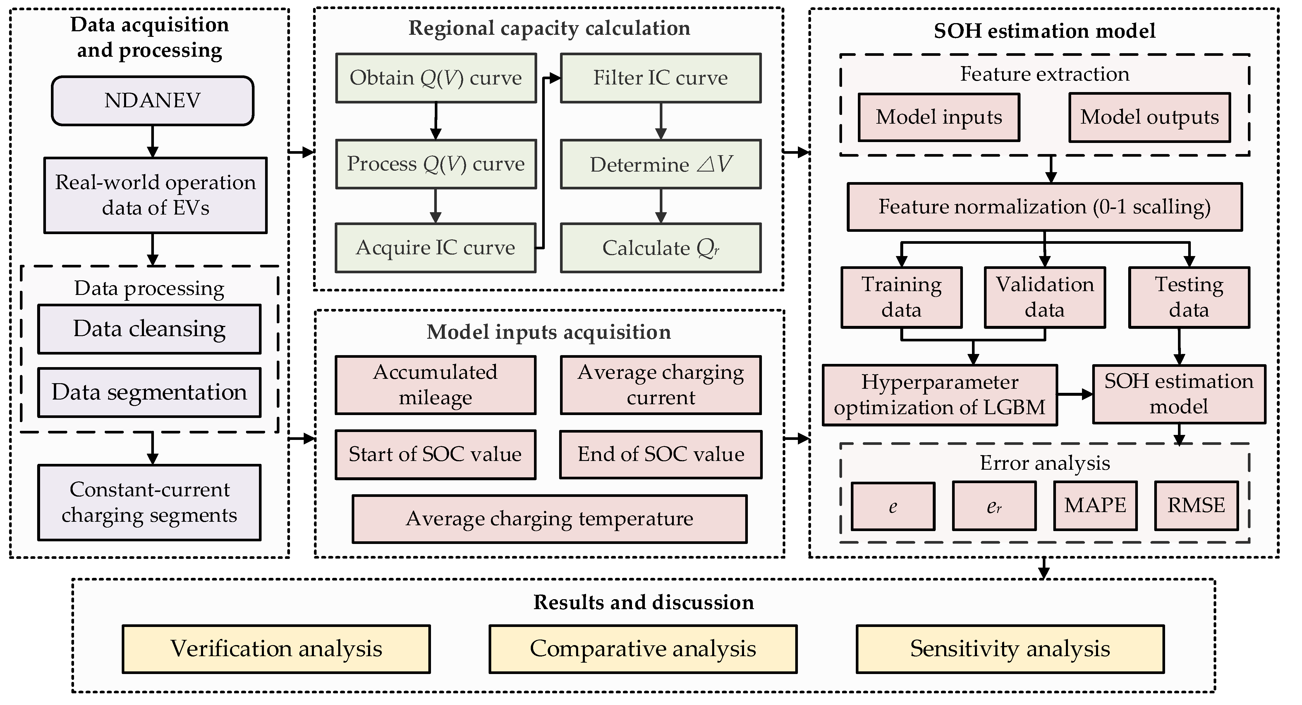
Figure 1. The framework diagram of SOH estimation.
Sustainability 15 02052 g001
Figure 2. (a) Current distribution and (b) SOC distribution during the charging process.
Sustainability 15 02052 g002
Figure 3. The voltage–capacity curve.
Sustainability 15 02052 g003
Figure 4. The IC curves: (a) the comparison of IC curves smoothed by the MA method; (b) the comparison of IC curves smoothed by the GS method.
Sustainability 15 02052 g004
Figure 5. The comparison of IC curves smoothed by the MA method and GS method.
Sustainability 15 02052 g005
Figure 6. The schematic diagram of the regional capacity.
Sustainability 15 02052 g006
Figure 7. The regional capacity evolution curves.
Sustainability 15 02052 g007
Figure 8. Schematic of the histogram-based algorithm.
Sustainability 15 02052 g008
Figure 9. Schematic of the tree growth strategies: (a) level-wise growth strategy; (b) leaf-wise growth strategy.
Sustainability 15 02052 g009
Figure 10. Framework of model construction.
Sustainability 15 02052 g010
Figure 11. Feature selection.
Sustainability 15 02052 g011
Figure 12. The MAPE under the variations of (a) the max depth and (b) the number of estimators.
Sustainability 15 02052 g012
Figure 13. Absolute error for the test datasets.
Sustainability 15 02052 g013
Figure 14. Relative error distribution for the test datasets.
Sustainability 15 02052 g014
Figure 15. SOH estimation results of test vehicle 1 based on (a) LR; (b) RF; (c) SVM; (d) LGBM.
Sustainability 15 02052 g015
Figure 16. SOH estimation results of test vehicle 2 based on (a) LR; (b) RF; (c) SVM; (d) LGBM.
Sustainability 15 02052 g016
Figure 17. SOH estimation results of test vehicle 3 based on (a) LR; (b) RF; (c) SVM; (d) LGBM.
Sustainability 15 02052 g017
Figure 18. SOH estimation results of test vehicle 4 based on (a) LR; (b) RF; (c) SVM; (d) LGBM.
Sustainability 15 02052 g018
Table 1. The specifications of the studied electric buses.
ParametersValue (Units)
Curb weight7800 kg
Number of battery cells336
Nominal voltage537.6 V
Nominal capacity240 Ah
Nominal energy129 kWh
Cathode materialsLiFePO4
Table 2. An example of the charging segment.
TimeAccumulated Mileage (km)Velocity (km/h)Battery System Voltage (V)Battery System Current (A)SOC (%)The Highest Temperature (°C)The Lowest Temperature (°C)
20190612091138156,334.40565.3−192863128
20190612091148156,334.40569.5−192863128
20190612091158156,334.40571.5−192863128
20190612092158156,334.40573.3−40993329
20190612092208156,334.40573.5−40993329
20190612092218156,334.40573.8−40993329
Table 3. An example of the driving segment.
TimeAccumulated Mileage (km)Velocity (km/h)Battery System Voltage (V)Battery System Current (A)SOC (%)The Highest Temperature (°C)The Lowest Temperature (°C)
2018010520270663,545.85553.116623023
2018010520271663,545.813551.933623023
2018010520272663,545.812552.917623023
20180105214356 63,570.83550.57522922
20180105214406 63,570.86550.52522922
20180105214416 63,570.95550.43522922
Table 4. MAPEs and RMSEs of SOH estimation.
VehicleLRRFSVMLGBM
MAPE (%)RMSE (%)MAPE (%)RMSE (%)MAPE (%)RMSE (%)MAPE (%)RMSE (%)
14.2542.2082.6591.4852.8381.7282.5201.403
21.7300.9471.9771.1172.0341.0781.5980.893
32.2471.2442.1871.1742.3631.2882.1581.164
41.8821.0862.0741.1682.5641.3621.8981.065
Test vehicles2.6121.5042.2391.2582.4521.3962.0491.153
Table 5. MAPEs and RMSEs with different noise rates.
Noise1%2%3%5%
MAPE (%)2.3542.4422.8392.881
RMSE (%)1.4011.3341.5691.663
Disclaimer/Publisher’s Note: The statements, opinions and data contained in all publications are solely those of the individual author(s) and contributor(s) and not of MDPI and/or the editor(s). MDPI and/or the editor(s) disclaim responsibility for any injury to people or property resulting from any ideas, methods, instructions or products referred to in the content.