Article

Relationship between Highway Geometric Characteristics and Accident Risk: A Multilayer Perceptron Model (MLP) Approach

1
National Engineering Laboratory of Land Traffic Meteorological Disaster Prevention and Control Technology, Yunnan Transportation Planning and Design Institute Co., Ltd., Kunming 6502001, China
2
Yunnan Key Laboratory of Digital Communications, Kunming 650103, China
3
School of Civil Engineering, Chongqing Jiaotong University, Chongqing 400074, China
4
School of Civil and Environmental Engineering, Nanyang Technological University, Singapore 639798, Singapore
*
Author to whom correspondence should be addressed.
These authors contributed equally to this work.
Sustainability 2023, 15(3), 1893; https://doi.org/10.3390/su15031893
Submission received: 16 November 2022 / Revised: 7 January 2023 / Accepted: 12 January 2023 / Published: 18 January 2023
(This article belongs to the Special Issue Transport Sustainability and Resilience in Smart Cities)

Abstract

:
The traffic safety of mountain highway has always been one of the taking point. This study aims to collect road design data in large-scale research and analyzes the accident risk of highway geometric alignment. Accordingly, a method based on satellite maps and clustering algorithms is proposed to calculate the geometric alignment of the highway plane and its longitudinal section. The reliability of the method was verified on Nanfu highway in Chongqing, China. The planar and longitudinal sectional geometries of the four highways in Chongqing were obtained by the above method, and the corresponding 36,439 traffic accidents which occurred from 2010 to 2016 were used as the research objects. The accident risk of the highway geometry was analyzed based on the SHAP and MLP theories. The results show that the fitting and prediction abilities of the MLP model are better than those of the negative binomial model, and its correlation coefficient is improved by 33.2%. In addition, compared with the negative binomial model, the MLP model can estimate more accurately and flexibly the complex nonlinear relationship between the independent and the dependent variables.

1. Introduction

Traffic safety is one of the major concerns in the world today. There are approximately 1.35 million deaths and over 50 million injuries every year due to traffic accidents worldwide [1]. In addition, it is estimated that low- and middle-income countries account for approximately 90% of the global total of road traffic fatalities [2]. As the world’s largest developing country, China has the highest population, car ownership, and total road mileage in the world, yet traffic safety still faces lots of challenges [3]. It is estimated that about one-fifth of traffic accidents are fatalities in China [4,5]. Therefore, the active investigation and management of traffic safety risks have become an urgent problem to be solved in building a green and sustainable highway traffic system.
Established research have shown that the main factors affecting traffic safety include people (drivers), vehicles, road conditions, and the environment, among which drivers are considered to have the greatest impact on traffic safety, while road conditions were often overlooked [6,7]. Road conditions affect the performance of moving vehicles, drivers’ psychological activities, and driving performance. Approximately 40% of traffic accidents were caused by direct or indirect influence of road conditions [8]. Babukov et al. studied the influence of highway horizontal and longitudinal cross-section alignment on traffic safety, and proposed recommendations for ensuring traffic safety in the stages of road design, operation, and maintenance [9]. Ma et al. analyzed the relationship between the design elements of road alignment (horizontal, longitudinal cross-section, and intersections) and the accident risk [10]. With the continuous development of the social economy, the current road design may become increasingly incapable of meeting the traffic demand today [11]. Therefore, it is necessary to analyze the contributory factors for traffic accidents under current road infrastructure conditions [12,13].
Many researchers used the traditional linear regression (LR) method to fit the relationship between road alignment, traffic volume and accident frequency, etc. However, some studies also found that the assumption of the linear regression with the Chi-square distribution of the variance is often violated in practical applications, and the unconstrained linear regression is not applicable to non-negative count models [14]. Subsequently, some scholars used Poisson regression to simulate the frequency of traffic accidents, and the results showed that its fitting effect is better than linear regression, but it was also found that accident data were too discrete and the model could not satisfy the assumption of equal mean and variance [15,16]. Miaou investigated the relationship between truck accidents and highway geometric features based on Poisson regression, zero-inflated Poisson regression (ZIP), and negative binomial regression (NB), and showed that ZIP and NB can handle the over-dispersion of accident data well [17]. Milton et al. used NB to study the relationship between accident frequency, road geometry as well as traffic characteristics and found that NB is a powerful tool for accident analysis [18]. Subsequently, some scholars successively applied generalized estimating equations, Bayesian, random effects, random parameters, etc., to the analysis of accident frequency [19,20].
Most traditional statistical models are parametric and are based on certain distribution assumptions. These models may have relatively robust predictive performance and good interpretability of the internal influence mechanism, but these models may be sensitive to data size, have poor real-time processing capability for big data, and cannot capture the complex nonlinear relationship between features and dependent variables [21,22,23].
Recently, machine learning has been widely applied to the research of traffic safety. Compared with traditional statistical models, machine learning models are able to approximate complex nonlinear relationships among multi-dimensional data variables and have unique advantages in real-time processing of big data and in the analyses of samples with complex structures. Therefore, they can flexibly respond to complex application scenarios and achieve high prediction accuracy [24]. Thakali et al. developed a parametric negative binomial model and a nonparametric kernel regression model based on a large amount of traffic accidents data and found that kernel regression outperformed the negative binomial model in terms of dataset size sensitivity [25]. The LSTM–CNN neural network model, was used by Li et al. for the prediction of real-time accident risks on arterial roads, and the results show that its prediction accuracy is better than other machine learning models such as XGBoost, LSTM, and CNN models [26]. Lee et al. compared and analyzed the difference in accuracy of different machine learning algorithms (random forest, MLP and decision tree) for rainfall traffic accident prediction [27]. Wang compared the modeling of accident risk in highway work zones using CNN and binary logistic regression models, respectively, and finally found that the CNN model had better accuracy [28].
At present, most of the road design documents in China are scattered in different design units and government agencies, which makes data acquisition difficult and not conducive to large-scale research. In this paper, we propose a road geometric alignment inverse calculation method by satellite map and clustering algorithm, which provides another solution for researchers. In addition, combining the characteristics of the data set, the author chooses the MLP model, which is more operable, to study the accident risk of highway geometric alignment, compare the results of the negative binomial model, and analyze the advantages and disadvantages of the nonlinear fit of the two in the correlation model. The internal mechanism of the MLP model is also visualized and analyzed with the help of SHAP theory, so as to compensate for the limited interpretability of machine learning algorithms.
In this study, firstly, the geometric alignment data of the target highway was calculated by the road geometric alignment inverse calculation method. Then, based on the traffic accident information of the target road, the MLP and negative binomial regression-based accident risk association models are established, respectively. Finally, the internal mechanism of the MLP model was visualized with the help of SHAP theory.

2. Methodology

2.1. Overall Framework

This paper aims to study the relationship between highway geometric characteristics and the risk of traffic accidents. To this end, the overall framework of the methodology is presented in Figure 1. There are four components in the overall framework: (1) Data survey, (2) Data preprocessing, (3) Model optimization, (4) contribution of variable.

2.2. Road Geometric Alignment Reverse Calculation

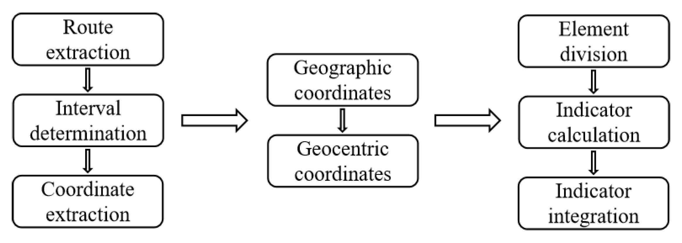
This section proposes an inverse calculation approach to extract the road geometric characteristics based on satellite maps, and the reliability of the approach is verified based on existing data. The process of inverse calculation approach is shown in Figure 2.
Firstly, for the extraction of routes and coordinates, most of the current map software can obtain the latitude and longitude of the target point and meet the required accuracy. In this study, Google Earth and Aowei interactive maps were used to mark the target routes and the longitude and latitude coordinates. Elevation information of each target point was also extracted at equal intervals. The longitude and latitude coordinates of the route were extracted at an interval of 10 m, and the elevation information was extracted at an interval of 40 m to balance the calculation accuracy and extraction efficiency.
Since the latitude and longitude coordinates provided by GPS are global coordinates (WGS84), the extracted latitude and longitude coordinates need to be converted to planar right-angle geodetic coordinates (WGS84). The coordinate conversion is performed by:
X = ν + c   c o s   ϕ   c o s   τ Y = ν + c   c o s   ϕ   s i n   τ Z = 1 e 2 ν + τ   s i n   ϕ
e 2 = a 2 b 2 a 2 = 2 f f 2
ν = a 1 e 2 s i n 2 ϕ
where X, Y, Z are global coordinate, ϕ is the latitude, τ is the longitude, c is the ellipsoidal height, ν is the radius of the doughnut circle at the latitude ϕ , e is the ellipsoidal eccentricity, a is the long semi-axis of the ellipsoidal model, b is the short axis of the ellipsoidal model, and f is the flatness of the ellipsoidal model.
Finally, based on the coordinate data and elevation information, the geometric characteristics of the road’s horizontal and longitudinal sections is back-calculated. The detailed steps are as follows.
(1)
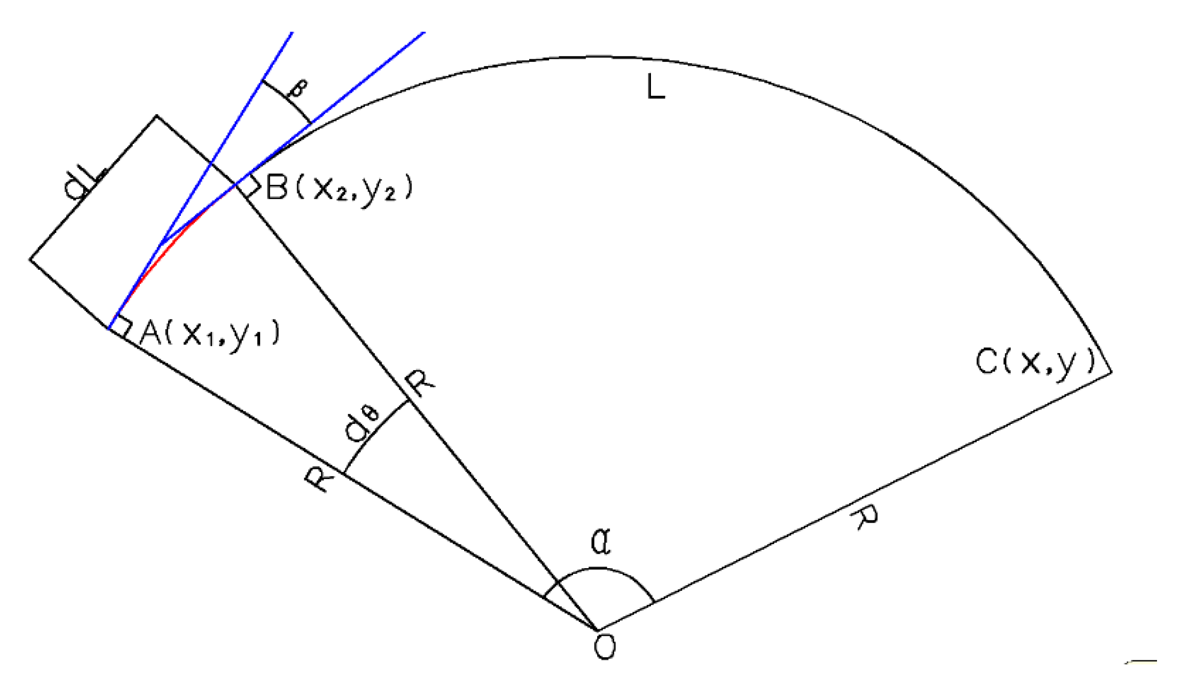
The road alignment is divided by means of microelement division (see Figure 3), with the horizontal and longitudinal section intervals being 10 m and 40 m, respectively. In Figure 3, the circular arc’s angle d θ and arc length d L i of the microelement segment i are calculated by:
d θ = β i = a r c t a n y i y i 1 x i x i 1     x i < x i 1 180 + a r c t a n y i y i 1 x i x i 1 x i > x i 1  
d l i = ( x i x i 1 ) 2 + ( y i y i 1 ) 2
(2)
The circular curve index is obtained by microelement integration. The final integrated flat curve deflection angle ( α ), flat curve length ( L ), and flat curve radius ( R ) are calculated by:
α = i = 1 n β i
L = i = 1 n d l i
R = 180 · L π · α
Due to the limited elevation data of the map software, the vertical curve alignment of the highway cannot be restored. In this study, with the limited elevation information, the terrain alignment of the highway is divided into uphill and downhill sections. The slope between adjacent points is calculated by:
g i = h i h i 1 d L i
When the slope is less than zero, the section is downhill, otherwise, it is regarded as an uphill section. In addition, when the slope exceeds ±8%, it is considered that this is either a bridge or tunnel section, and the value was replaced by ±1%.

2.3. Negative Binomial Regression

Negative binomial regression can be understood as Poisson regression in a generalized sense, by introducing a gamma noise term enabling the model to deal with overdispersion of accident data [29,30]. Negative binomial regression relaxes the assumption of equal expectation and variance in the Poisson distribution by introducing an error term ε i [31], and the expression for the average accident number λ i of road section cells is as follows:
λ i = t i e β X i + ε i
In Equation (10), e β X i + ε i is the data that obeys a gamma distribution with a mean equal to one and a variance equal to . The probability of the negative binomial model can be written:
P n i = Γ n i + α 1 Γ α 1 · n i ! 1 1 + α λ i α 1 α λ i 1 + α λ i n i

2.4. Multilayer Perceptron Model

The multilayer perceptron model is based on the theoretical extension of the perceptron model proposed by Rosenblatt in the 1950s [32]. Perceptual machines are capable of handling linearly divisible problems of simple logic (such as with, or, and without). However, it has only one layer of functional neurons with limited ability to solve nonlinear separable problems. The multilayer perceptron solves the above problem by adding several layers of functional neurons between the input and output layers. The schematic is shown below [33].
Figure 4 shows that each layer of the multilayer perceptron is fully interconnected with the subsequent layer of neurons, and there are neither same-layer connections between neurons nor any cross-layer connections. The input layer does not contain functional neurons but only serves as a structural unit to receive information. The neurons in the implicit and output layers need to process the signals transmitted from the input layer, and the final results are derived from the output layer.
Assume that the training set is D = ( x 1 , y 1 ) , x 2 , y 2 , , ( x N , y N ) , x i R d , y i R l . That is, the input layer consists of a total of d neurons, and the output dimension is a n-dimensional vector. Additionally, assume that the hidden layer is a single-layer structure consisting of q neurons, the threshold of the jth neuron in the output layer is ξ j , and that the threshold of the hth neuron of the middle hidden layer is λ h ; v i h is the connection weight between the ith neuron in the input layer and the hth neuron in the hidden layer, v i h and w i h is the connection weight between the hth neuron of the hidden layer and the jth neuron of the output layer. The ReLU function was chosen as the activation function. In addition, α h is the input of the hth neuron of the middle layer, β j is the input of the hth neuron in the output layer, and y j is the output. The relevant calculations are below.
α h = i = 1 d v i h x i ,
β j = h = 1 q w h j b h ,
y j = f h = 1 q w h j · b h + ζ j ,
The multilayer perceptron solves the problem of assigning a weighting factor by using an error back-propagation algorithm. The core of the algorithm is to minimize the cumulative error on the training set, where the mean-square error on the nth sample is denoted by E n :
E n = 1 2 j = 1 l y j n y ^ j n 2

2.5. SHAP Interpretation

The SHAP model is often used to interpret the importance of features of complex models, such as deep learning models [34]. Due to its powerful parsing and visualization capability, some scholars have gradually applied it to the study of traffic safety in recent years [35,36]. The expression of the SHAP model is as follows.
g z = φ 0 + i = 1 M φ i z i
where g · represents the interpreter, φ 0 represents the model benchmark, φ i is the Shapley value of the first feature, M represents the number of features, and z i indicates the presence or absence of this feature.

2.6. Model Evaluation Metrics

In this study, the overall relative error (ORE), mean absolute deviation (MAD), cumulative residual (CSR), and correlation coefficient ( ρ Y , Y ) metrics are chosen to evaluate the prediction accuracy and generalization performance of each model.
O R E = y ¯ i y ¯ i y ¯ i
M A D = 1 n i = 1 n y i y i
C S R = i = 1 n y i y i y i + k y i 2
ρ Y , Y = c o v Y , Y σ Y σ Y
where y i and y i the true and predicted accident frequencies of the ith road section, respectively, and n is the number of road sections.

3. Results

3.1. Traffic Accident Data

In this study, data and information pertaining to 36,439 traffic accidents from 2010 to 2016 were collected from the traffic management department of Chongqing, China, for four highways with a total statistical mileage of up to 1194.8 km. The accident information mainly includes the time of the incident, driver information, location of the incident, casualty information, weather conditions, accident patterns, the topography of the accident, road conditions, traffic control mode, road type, road alignment, lighting conditions, accident category, etc. The statistical information of each highway accident is tabulated in Table 1.

3.2. Verification of Road Geometric Alignment Backcalculation

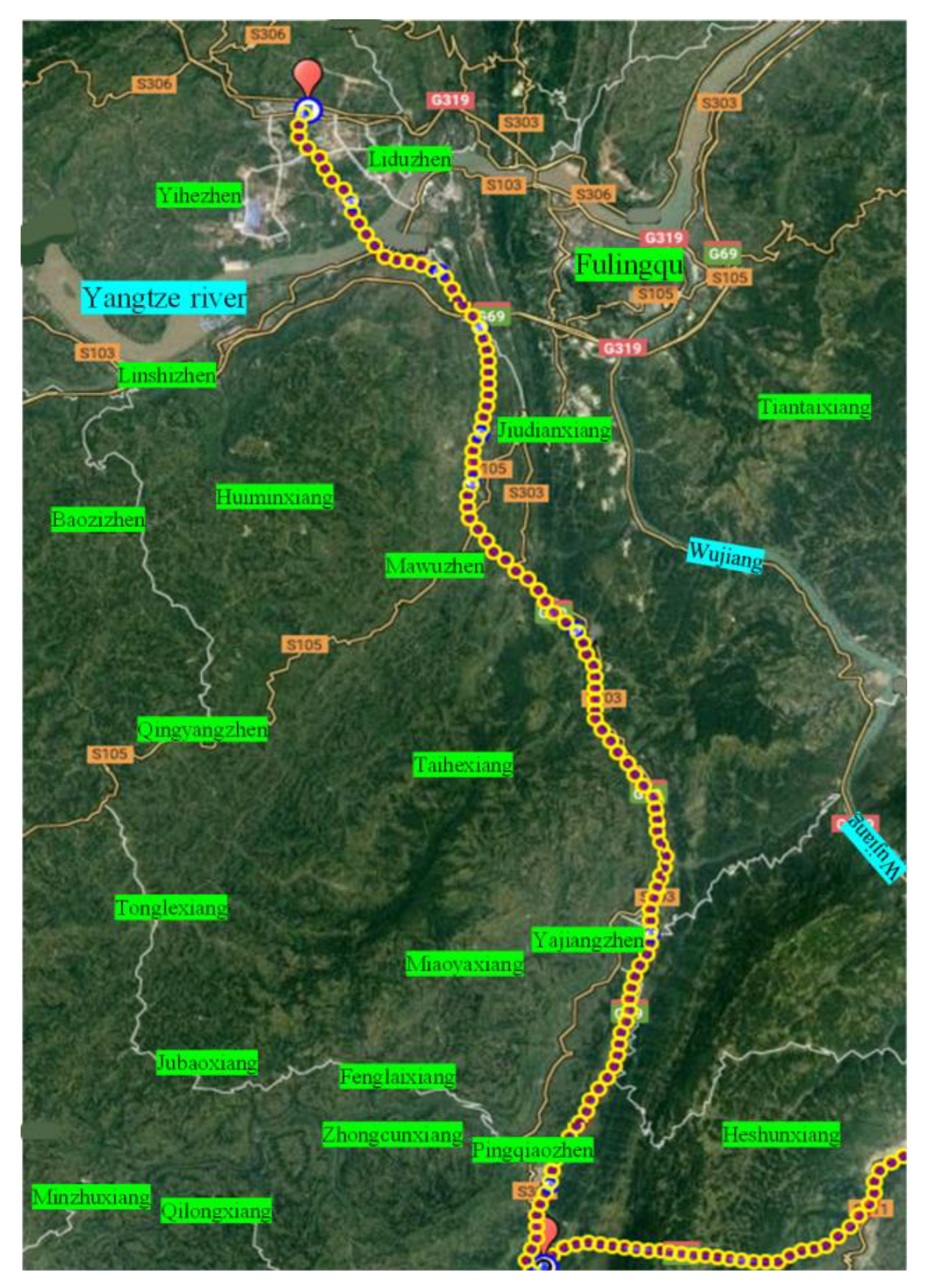
The reliability of the back-calculation method was verified by using a part of the Nanfu highway in Chongqing, China, which had a total mileage equal to 55 km (see Figure 5). The longitude, latitude, and elevation information of each target point along the route were extracted at intervals of 10 m and 40 m, respectively. According to the calculation process (see Equations (4)–(9)), microelement calculation was conducted to obtain the final inverse calculation results of the highway plane and longitudinal section alignment index. The result of the validation is listed in Table 2.
From Table 2, the correlation coefficients of the flat curve’s length, flat curve deflection angle, longitudinal slope length, and longitudinal slope gradient are all above 0.85. It shows that the calculated values are consistent with the design values. However, the correlation coefficient between the design and calculated values of the flat curve radius is only 0.3, and the statistical result shows that the difference between the calculated and the maximum value of the design flat curve’s radius is significant (see Table 3, the error is 64.94%). Then, the K-means clustering algorithm was used to further cluster the flat curve radius indices. There are three outliers in the inverse calculation values of 8.26 km, 8.80 km, and 11.29 km, which are much larger than the design value of this indicator for the corresponding road section. After removing these three resultant points, the correlation index between the design and calculated values of the flat curve radius will rise to 0.72, and the corresponding value will be less than 0.0001, thus indicating that they are significantly correlated. Therefore, the road geometric alignment back calculation algorithm can be used for subsequent traffic safety prediction analysis.

3.3. Model Fitting Results

According to the calculated geometric alignment results, the homogeneous method was then used to divide the road into several section units. A total of 2063 road section units were finally obtained as the basic data for the study. The section unit length, straight section length, flat curve radius, flat curve deflection angle, longitudinal slope gradient, longitudinal slope length, and slope difference were selected as the input variables of the model. The section unit accident frequency was used as the explanatory variable of the model. In order to avoid too large variables that may result in very small intervals, the study readjusted the unit of each input variable (Table 4). Additionally, it was assumed that the flat curve radius and flat curve deflection angle of the straight section unit were 100 km (infinity) and 0°, respectively. The length of the straight section on the flat curve section was 0 km.
A randomly selected part (80%) of the data constituted the training set for the training and parameter calibration of the MLP model. The remaining 20% of the data was used to validate the generalization performance of the model. Besides, a negative binomial regression model was used as a control method to analyze the differences between the traditional statistical method and the machine learning method. The accuracy of the negative binomial model and MLP model predictions were evaluated based on the ORE, MAD, CSR, ρY,Y′. The implementation process of MLP model hyperparameter optimization is shown as follows:
(1)
Determining the MLP model input and output dimensions as well as formulating the number of neurons in the input and output layers.
(2)
To speed up the convergence of the MLP model, the data set needs to be normalized and compressed into a finite value domain space.
(3)
Importing the normalized accident data into the MLP model, determining the cost function of the neural network model, and calibrating the hyperparameters of the multilayer perceptron model until the model reaches the target accuracy.
(4)
Importing normalization of the fitted prediction results of the MLP to restore the original magnitude of the data. The optimization of the hyperparameters of the MLP model are shown in Table 5 and A comparison between negative binomial model and MLP model is outlined in Table 6.
For the negative binomial model, the magnitude of the absolute value of the regression parameters could indicate indirectly the degree of influence of the explanatory variables on the dependent variable. The RI value in the MLP model results is the relative importance of the feature calculated by SHAP theory, and the larger the value, the higher the contribution of the feature to the explanatory variables. From the results, it can be observed that the negative binomial model is consistent with the determined MLP model for the feature with the greatest degree of influence on the frequency of roadway accidents, that is, the roadway unit length; its corresponding RI value in the MLP is equal to 0.151. However, the importance ranking of subsequent features in the MLP model is slightly different from that of the negative binomial model, where the subsequent ranking in the negative binomial model is Sl > Hcr > Vl > Hca . The ranking in the MLP model calculation results is Hcr > Hca > Sl > Vl > Vcg > Gd . In addition, the explanatory variables in the negative binomial model that are significantly related to the dependent variable also have the highest RI values in the MLP model.
The overall relative errors of the negative binomial model and the multilayer perceptron model are approximately the same (both are about 3%).
However, the mean absolute deviation, cumulative residuals and correlation coefficients of the multilayer perceptron model are better than those of the negative binomial regression model, thus indicating that the multilayer perceptron model has a better prediction performance for the frequency of accidents in mountainous highway sections than that of the negative binomial model.

3.4. Variable Correlation Analysis

As a type of parametric statistical model, the negative binomial model has good explanatory properties, and the effect of its explanatory variables on the dependent variable can be analyzed according to the nature of its regression coefficients. From Table 6, the road section unit length, straight section length, and longitudinal slope length are all greater than zero, thus indicating a positive correlation between these three characteristic variables and the accident frequency of the selected road sections. Thus, it can be concluded that the accident frequency gradually increases as these three characteristic variables increase. By contrast, the flat curve radius and flat curve deflection angle are negatively correlated with the frequency of road unit accidents.
This paper further explored the nonlinear relationships between the six independent variables ranked high in relative importance and the dependent variables in the MLP model through SHAP theory. The independent variables are the road section unit length, flat curve radius, flat curve deflection angle, straight-line section length, slope length, and slope degree.
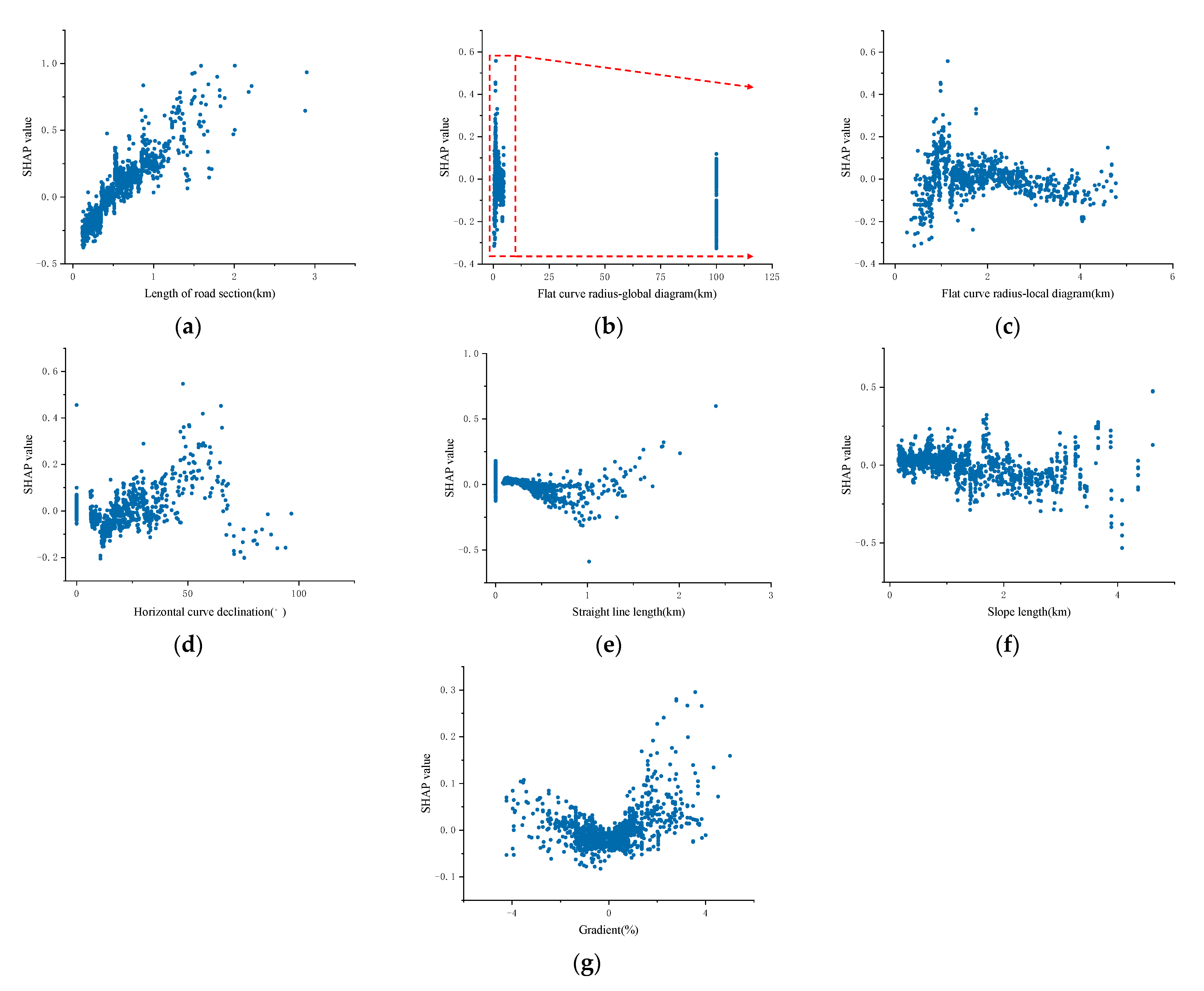
Figure 6a shows that there is a positive correlation between the length of the road section unit and the accident frequency within the road section, and the greater the length of the road section is, the higher the accident risk within the road section will be. In addition, it can also be observed that the accident risk increases as a function of the road section unit length as a Log function, and the growth rate gradually decreases. The SHAP dependence plots of the flat curve radius and accident frequency of roadway units are shown in Figure 6b,c. The radius of the flat curve of the straight-line section was set to 100 km to ensure the operation of the model; thus, there is a sample clustering point at the location of 100 km in Figure 6b, where in the sample points are all straight-line section units. Figure 6c shows that there is not a simple linear relationship between the radius of the road section unit flat curve and the frequency of accidents within the unit. The relationship is such that at the beginning, as the radius of the road section flat curve increases, the accident frequency within the unit gradually decreases, while in instances in which the radius of the road section unit flat curve exceeds about 3.9 km, the accident risk within the unit increases slightly. The conclusion here is not entirely consistent with the established studies in which the radius of a flat curve is negatively correlated with the frequency of unit accidents on flat curve sections [37]. The reason for this analysis is attributed to the fact that long and straight sections can have an impact on driving safety. When the radius of the flat curve is too large, the curvature of the flat curve is relatively small, and the driving difficulty is low; therefore, the driver is prone to subconsciously increase the speed, thus increasing the risk of accidents.
There are two inflection points in the data in Figure 6d. The results indicate a higher-order polynomial correlation between the deflection angle of the flat curve and the frequency of roadway unit accidents. When the flat curve deviation angle of the road section is less than 19° or more than 60°, the accident frequency is negatively correlated with the flat curve deviation angle, and the accident risk gradually decreases as a function of the flat curve deviation angle in this interval section. In addition, when the flat curve deflection angle is between the two inflection points, the accident risk of the road section increases in relation to the increase of the flat curve deflection angle. The conclusion is consistent with established studies in terms of the pattern of change, except for the difference in threshold values.
Figure 6e shows that the accident frequency of the road section at the beginning gradually decreases as a function of straight-line length, and there is a quadratic polynomial relationship between the straight-line length and the accident frequency. When the straight-line length exceeds 1.15 km, the length of the straight-line section is positively correlated with the accident risk. That is, when the straight-line length within the section is too short or too long, are not conducive to highway traffic safety.
Figure 6f shows that the frequency of accidents within the road section decreases as a function of the increase in slope length. However, when the slope length exceeds 2.8 km, the accident risk in the road section increases slightly as a function of the slope length. Analyzing the reason is that the car would brake frequently and easily in the long downhill section, thus leading to overheating of the brake system and a decrease in braking performance, which is not conducive to driving safety. For the long uphill section, the travel speed of large vehicles is reduced considerably, thus leading to increases in the speed differences between large vehicles and small vehicles; in turn, this leads to an increase in the frequency of overtaking, thus increasing the risk of traffic accidents.
Figure 6g shows the SHAP dependence of the longitudinal slope gradient and accident frequency, from which it can be observed that the longitudinal slope gradient is correlated with the accident frequency based on a quadratic polynomial function. The accident risk of the road unit gradually increases as a function of the increase of the absolute value of the longitudinal slope, and the rate of increase of accident risk on the uphill slope is slightly larger than that on the downhill slope. This study found that the accident risk of road section units gradually increases with the increase of the absolute value of longitudinal slope, and the rate of accident risk increase on uphill is slightly larger than that on downhill. This conclusion differs from the studies [37] in which the number of accidents on downhill sections is relatively higher than the number of accidents on uphill sections for the same absolute value of slope.

4. Conclusions

This study aims to collect road design data in large-scale research and analyzes the accident risk of highway geometric alignment. Accordingly, a method based on satellite maps and clustering algorithms is proposed to calculate the geometric alignment of the highway plane and its longitudinal section and the reliability of the method was verified on Nanfu highway in Chongqing, China. With the corresponding 36,439 traffic accidents which occurred from 2010 to 2016 being used as the research objects. The accident risk of the highway geometry was analyzed based on the SHAP and MLP theories. The conclusions are as follows:
(1)
A set of back-calculation methods based on a microelement method and cluster analysis of road geometric alignment was proposed in this study, and a 55 km highway was selected to verify the reliability of the method. The results showed that the back-calculated values of the flat curve length, flat curve deflection angle, longitudinal slope length, and longitudinal slope gradient were significantly correlated with the designed values. In addition, the correlation between the back-calculated values of the flat curve radius and the design value was improved significantly after stripping the outliers based on cluster analysis.
(2)
The section unit length, straight-line segment length, flat curve radius, flat curve deflection angle, longitudinal slope gradient, longitudinal slope length, and slope difference were selected as the input variables of the model, and the fitted prediction models were established by using the negative binomial regression and multilayer perceptron algorithm. Furthermore, the prediction accuracy of the model was evaluated by using the overall relative error, mean absolute deviation, cumulative residual, and correlation coefficient. The results showed that the prediction accuracy of the MLP model was better than that of the negative binomial model, and the evaluation indices were 3.2%, 0.371, 193.38, and 0.581, respectively.
(3)
SHAP theory was used to visualize the internal mechanism of action of the MLP model, and the results showed that only the road section unit length was monotonically and positively correlated with the accident frequency; the other characteristic variables exhibited complex nonlinear relationships with the accident frequency. Compared with the negative binomial model, the MLP model can estimate the complex nonlinear relationship between the independent and dependent variables more accurately and flexibly and can thus obtain a higher prediction accuracy.
(4)
In a future study, a comprehensive evaluation of road infrastructure accident risks will be conducted by introducing additional features, such as traffic flow and road cross-sections.

Author Contributions

J.Y. and S.Z. both contributed equally to this work and designated as co-first authors. Conceptualization, J.Y. and S.Z.; methodology, W.Y. and B.T.; investigation, Y.C. and F.Z.; writing—review and editing, J.Y. and S.Z. All authors have read and agreed to the published version of the manuscript.

Funding

This work was jointly funded by the science and technology innovation program of the department of transportation, Yunnan province, China (No. 2019303 and 2021-90-2), the general program of natural science foundation, Yunnan province, China (No 2019FB072), the general program of key science and technology in transportation, the ministry of transport, China (No. 2018-MS4-102), and the National Engineering Laboratory Open Research Fund Project for Land Traffic Meteorological Disaster Prevention and Control Technology of China (NEL-2020-01).

Institutional Review Board Statement

Not applicable.

Informed Consent Statement

Not applicable.

Data Availability Statement

Not applicable.

Conflicts of Interest

The authors declare no conflict of interest.

References

  1. Shah, S.A.R.; Ahmad, N.; Shen, Y.; Pirdavani, A.; Basheer, M.A.; Brijs, T. Road safety risk assessment: An analysis of transport policy and management for low-, middle-, and high-income Asian countries. Sustainability 2018, 10, 389. [Google Scholar] [CrossRef] [Green Version]
  2. World Health Organization. Global Status Report on Road Safety 2018: Summary; World Health Organization: Geneva, Switzerland, 2018. [Google Scholar]
  3. Fayard, G. Road injury prevention in China: Current state and future challenges. J. Public Health Policy 2019, 40, 292–307. [Google Scholar] [CrossRef]
  4. Wang, X.; Yu, H.; Nie, C.; Zhou, Y.; Wang, H.; Shi, X. Road traffic injuries in China from 2007 to 2016: The epidemiological characteristics, trends and influencing factors. PeerJ 2019, 7, e7423. [Google Scholar] [CrossRef] [Green Version]
  5. Wang, C.; Quddus, M.A.; Ison, S.G. The effect of traffic and road characteristics on road safety: A review and future research direction. Saf. Sci. 2013, 57, 264–275. [Google Scholar] [CrossRef]
  6. Lord, D.; Qin, X.; Geedipally, S. Highway Safety Analytics and Modeling; Elsevier: Amsterdam, The Netherlands, 2021. [Google Scholar]
  7. Horberry, T.; Anderson, J.; Regan, M.A.; Triggs, T.J.; Brown, J. Driver distraction: The effects of concurrent in-vehicle tasks, road environment complexity and age on driving performance. Accid. Anal. Prev. 2006, 38, 185–191. [Google Scholar] [CrossRef]
  8. Babkov, V.F. Road Conditions and Traffic Safety; National Academy of Sciences: Washington, DC, USA, 1975. [Google Scholar]
  9. Pei, Y.; Ma, J. Transport. Research on countermeasures for road condition causes of traffic accidents. China J. Highw. Transp. 2003, 16, 77–82. [Google Scholar]
  10. Ji, M.; Jiang, B.; Chen, S.; Li, H. Design and Research of Civil Engineering Courses under the Guidance of “The Belt and Road” Strategy Based on Craftsman Spirit. In Proceedings of the 2019 International Conference on Management, Education Technology and Economics (ICMETE 2019), Fuzhou, China, 25–26 May 2019; pp. 492–495. [Google Scholar]
  11. Zhao, L.; Liu, Z.; Mbachu, J. Highway alignment optimization: An integrated BIM and GIS approach. ISPRS Int. J. Geo-Inf. 2019, 8, 172. [Google Scholar] [CrossRef] [Green Version]
  12. Pei, Y.-L.; He, Y.-M.; Ran, B.; Kang, J.; Song, Y.-T. Horizontal Alignment Security Design Theory and Application of Superhighways. Sustainability 2020, 12, 2222. [Google Scholar] [CrossRef] [Green Version]
  13. Jovanis, P.P.; Chang, H.-L. Modeling the relationship of accidents to miles traveled. Transp. Res. Rec. 1986, 1068, 42–51. [Google Scholar]
  14. Joshua, S.C.; Garber, N.J. Estimating truck accident rate and involvements using linear and Poisson regression models. Transp. Plan. Technol. 1990, 15, 41–58. [Google Scholar] [CrossRef]
  15. Miaou, S.-P.; Hu, P.S.; Wright, T.; Rathi, A.K.; Davis, S.C. Relationship between truck accidents and highway geometric design: A Poisson regression approach. Transp. Res. Rec. 1992, 10–18. [Google Scholar]
  16. Miaou, S.-P. The relationship between truck accidents and geometric design of road sections: Poisson versus negative binomial regressions. Accid. Anal. Prev. 1994, 26, 471–482. [Google Scholar] [CrossRef] [PubMed] [Green Version]
  17. Milton, J.; Mannering, F. The relationship among highway geometrics, traffic-related elements and motor-vehicle accident frequencies. Transportation 1998, 25, 395–413. [Google Scholar] [CrossRef]
  18. Lord, D.; Mannering, F. The statistical analysis of crash-frequency data: A review and assessment of methodological alternatives. Transp. Res. Part A Policy Pract. 2010, 44, 291–305. [Google Scholar] [CrossRef] [Green Version]
  19. Wang, C.; Chen, F.; Cheng, J.; Bo, W.; Zhang, P.; Hou, M.; Xiao, F. Random-Parameter Multivariate Negative Binomial Regression for Modeling Impacts of Contributing Factors on the Crash Frequency by Crash Types. Discret. Dyn. Nat. Soc. 2020, 2020, 6621752. [Google Scholar] [CrossRef]
  20. Ferreira-Vanegas, C.M.; Vélez, J.I.; García-Llinás, G.A. Analytical methods and determinants of frequency and severity of road accidents: A 20-year systematic literature review. J. Adv. Transp. 2022, 2022, 7239464. [Google Scholar] [CrossRef]
  21. Islam, A.; Haque, B.; Hasan, J.; Amin, R. Frequency Modelling and Risk Evaluation of Road Crashes in Sylhet Region of Bangladesh. Int. J. Intell. Transp. Syst. Res. 2021, 20, 90–102. [Google Scholar] [CrossRef]
  22. Theofilatos, A. Utilizing Real-time Traffic and Weather Data to Explore Crash Frequency on Urban Motorways: A Cusp Catastrophe Approach. Transp. Res. Procedia 2019, 41, 471–479. [Google Scholar] [CrossRef]
  23. Wu, P.; Meng, X.; Song, L. A novel ensemble learning method for crash prediction using road geometric alignments and traffic data. J. Transp. Saf. Secur. 2019, 12, 1128–1146. [Google Scholar] [CrossRef]
  24. Thakali, L.; Fu, L.; Chen, T. Model-Based Versus Data-Driven Approach for Road Safety Analysis: Do More Data Help? Transp. Res. Rec. J. Transp. Res. Board 2016, 2601, 33–41. [Google Scholar] [CrossRef]
  25. Li, P.; Abdel-Aty, M.; Yuan, J. Real-time crash risk prediction on arterials based on LSTM-CNN. Accid. Anal. Prev. 2020, 135, 105371. [Google Scholar] [CrossRef]
  26. Lee, J.; Yoon, T.; Kwon, S.; Lee, J. Model Evaluation for Forecasting Traffic Accident Severity in Rainy Seasons Using Machine Learning Algorithms: Seoul City Study. Appl. Sci. 2019, 10, 129. [Google Scholar] [CrossRef] [Green Version]
  27. Wang, J.; Song, H.; Fu, T.; Behan, M.; Jie, L.; He, Y.; Shangguan, Q. Crash prediction for freeway work zones in real time: A comparison between Convolutional Neural Network and Binary Logistic Regression model. Int. J. Transp. Sci. Technol. 2022, 11, 484–495. [Google Scholar] [CrossRef]
  28. Lambert, D. Zero-inflated Poisson regression, with an application to defects in manufacturing. Technometrics 1992, 34, 1–14. [Google Scholar] [CrossRef]
  29. Winkelmann, R. Seemingly unrelated negative binomial regression. Oxf. Bull. Econ. Stat. 2000, 62, 553–560. [Google Scholar] [CrossRef]
  30. Hilbe, J. Negative Binomial Regression; Cambridge University Press: Cambridge, UK, 2011. [Google Scholar]
  31. Rosenblatt, F. The Perceptron, a Perceiving and Recognizing Automaton Project Para; Cornell Aeronautical Laboratory: Buffalo, NY, USA, 1957. [Google Scholar]
  32. Velo, R.; López, P.; Maseda, F. Wind speed estimation using multilayer perceptron. Energy Convers. Manag. 2014, 81, 1–9. [Google Scholar] [CrossRef]
  33. Lundberg, S.M.; Lee, S.-I. A unified approach to interpreting model predictions. In Proceedings of the 31st International Conference on Neural Information Processing Systems, Red Hook, NY, USA, 4–9 December 2017; p. 30. [Google Scholar]
  34. Yang, C.; Chen, M.; Yuan, Q. The application of XGBoost and SHAP to examining the factors in freight truck-related crashes: An exploratory analysis. Accid. Anal. Prev. 2021, 158, 106153. [Google Scholar] [CrossRef]
  35. Parsa, A.B.; Movahedi, A.; Taghipour, H.; Derrible, S.; Mohammadian, A.K. Toward safer highways, application of XGBoost and SHAP for real-time accident detection and feature analysis. Accid. Anal. Prev. 2020, 136, 105405. [Google Scholar] [CrossRef]
  36. Ribeiro, M.T.; Singh, S.; Guestrin, C. “Why should i trust you?” Explaining the predictions of any classifier. In Proceedings of the 22nd ACM SIGKDD International Conference on Knowledge Discovery and Data Mining, San Francisco, CA, USA, 13–17 August 2016; pp. 1135–1144. [Google Scholar]
  37. Štrumbelj, E.; Kononenko, I. Explaining prediction models and individual predictions with feature contributions. Knowl. Inf. Syst. 2014, 41, 647–665. [Google Scholar] [CrossRef]
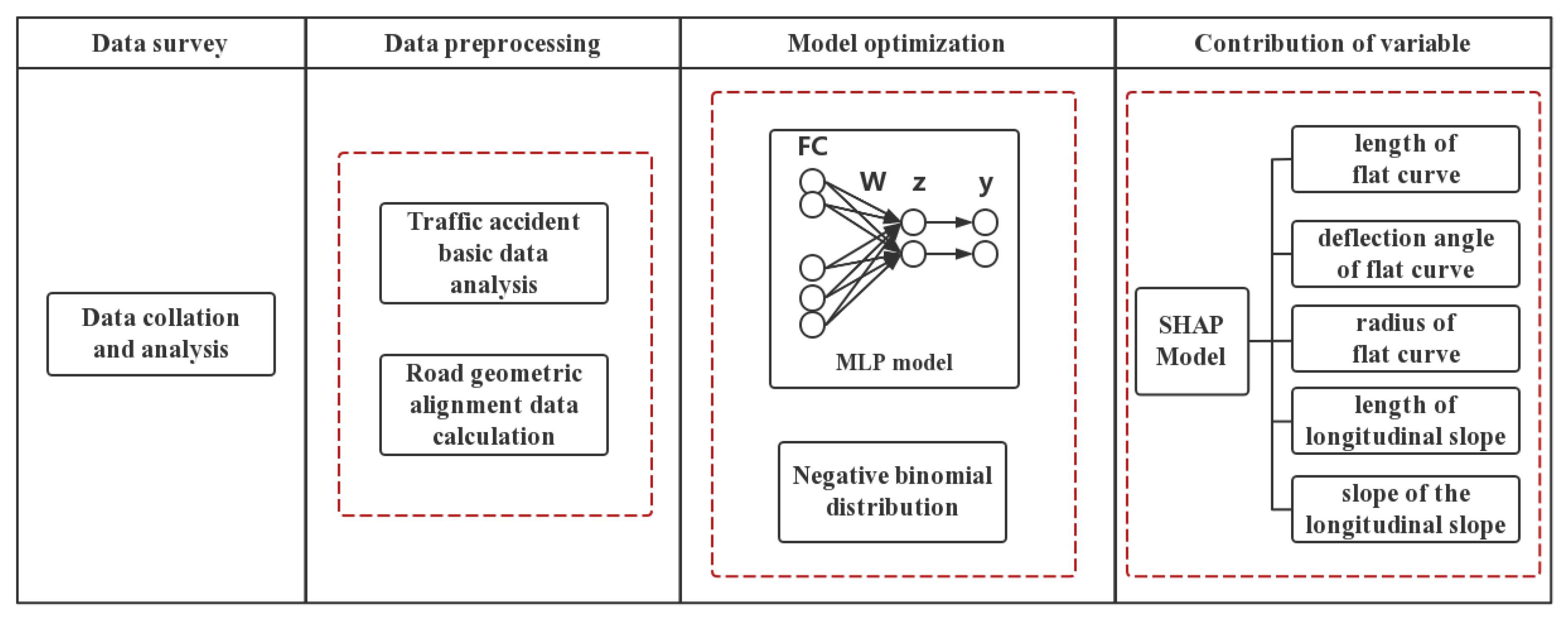
Figure 1. Overall framework of the methodology.
Sustainability 15 01893 g001
Figure 2. Inverse calculation process used for geometric alignment data extraction.
Sustainability 15 01893 g002
Figure 3. Schematic of microelement calculation of a circular arc.
Sustainability 15 01893 g003
Figure 4. Schematic of multilayer perceptron.
Sustainability 15 01893 g004
Figure 5. Nanchuan–Fuling Highway satellite map determination.
Sustainability 15 01893 g005
Figure 6. Plots of the SHapley Additive exPlanations values of various input variables: (a) length of the road section; (b) flat curve radius; (c) zoom plot of plot b; (d) flat curve deflection angle; (e) length of straight-line section; (f) length of slope; (g) slope gradient.
Sustainability 15 01893 g006
Table 1. Statistics of traffic accidents on four highways studied herein from 2010 to 2016.
Road SectionStatistical Mileage/kmNumber of AccidentsNumber of DeathsNumber of InjuredDirect Property Damage/Million Yuan
Baomao highway501.17483246240513,248
Hulong highway352.52455948032156
Lanhai highway22913,404138198817,196
Yinkun highway112.213,09785175511,374
Total1194.836,439563695143,974
Only the information pertaining to the four highways in Chongqing City listed above was considered.
Table 2. Correlation test results.
Calculated ValuesDesign Value
Length of Flat CurveDeflection Angle of Flat CurveRadius of Flat CurveLength of Longitudinal SlopeSlope of the Longitudinal Slope
length of flat curve0.89 **−0.290.03
deflection angle of flat curve−0.140.96 **−0.52 **
radius of flat curve0.06−0.33 *0.30
length of longitudinal slope0.95 **0.05
slope of the longitudinal slope0.100.94 **
** Represents significant correlation at the 0.001 level; * represents significant correlation at the 0.05 level.
Table 3. Statistical analysis of the calculated and design values of the horizontal curve radius.
Radius of Flat CurveMaximum (/km)Average Value (/km)Minimum (/km)Error (/%)
calculated values11.292.540.5664.94
design value3.601.540.79
Table 4. Summary statistics of variables.
Independent VariableVariable SymbolsUnitAverage ValueStandard DeviationMinimum ValueMaximum Value
accident frequency-several cases per year0.480.5202.57
length of road sectionLkm0.510.330.122.9
length of straight sectionSlkm0.170.2702.4
flat curve radiusHcr10 km3.524.650.013610
deflection angle of flat curveHca°14.6318.26097.83
longitudinal slope gradientVcg%1.263.71−4.24.
longitudinal slope lengthVlkm1.220.920.154.6
slope differenceGd%1.694.7108.7
Table 5. Hyperparameters Tuning.
HyperparameterRangeValue
Learning Rate0.00001, 0.0001, 0.001, 0.01, 0.10.001
Batch Size16, 32, 6432
Optimization FunctionSGD,Adam,RMSpropAdam
Number of hidden layers2, 4, 6, 84
Number of monolayer neurons40, 60, 80, 100, 120, 140120
Maximum number of iterations250, 300, 350, 400, 450, 500450
Table 6. Model result comparison.
Negative Binomial ModelMLP
VariablesCoefficientStandard ErrORp ValueRIRank
L0.9310.0780.0000.1511
Sl0.1570.0760.0390.0354
Vcg−0.1130.7510.8800.0226
Hcr−0.0500.0080.0000.0532
Vl0.0480.0190.0120.0265
Gd0.0100.6520.9870.0177
Hca−0.0040.0020.0410.0453
_cons−1.1230.0600.000————
α0.1510.041——————
Evaluation metrics
ORE3.5%3.2%
MAD0.4410.371
CSR216.609193.380
ρY,Y′0.4360.581
Note: p-values less than 0.05 indicate that the variable is significantly correlated with the dependent variable. RI: Related importance = mean (|SHAP value|).
Disclaimer/Publisher’s Note: The statements, opinions and data contained in all publications are solely those of the individual author(s) and contributor(s) and not of MDPI and/or the editor(s). MDPI and/or the editor(s) disclaim responsibility for any injury to people or property resulting from any ideas, methods, instructions or products referred to in the content.