Empirical Study of the Effect of Thermal Loading on the Heating Efficiency of Variable-Speed Air Source Heat Pumps

Abstract

Heating buildings with air source heat pumps (ASHPs) has the potential to save energy compared to utilizing conventional heat sources. Accurate understanding of the efficiency of ASHPs is important to maximize the energy savings. While it is well understood that, in general, ASHP efficiency decreases with decreasing outdoor temperature, it is not well understood how the ASHP efficiency changes with different levels of thermal loading, even though it is an important consideration for sizing and controlling ASHPs. The goal of this study was to create an empirical model of the ASHP efficiency as a function of two independent variables–outside temperature and level of thermal loading. Four ductless mini-split ASHPs were evaluated in a cold chamber where the temperature (representing the outdoor temperature) was varied over a wide range. For each temperature, the ASHP performance data were collected at several levels of thermal loading. The data for all four ASHPs were combined and approximated with an analytical function that can be used as a general model for the ASHP steady-state efficiency as a function of the outside temperature and level of thermal loading. To the knowledge of the authors, no such empirical model that is solely based on third-party test data has been published before. While limitations exist, the model can be used to help guide future selection and operation of ASHPs.

1. Introduction

Almost 90% of the world’s primary energy comes from non-renewable sources [1], which poses a major challenge with respect to the sustainability of current energy practices. The use of energy efficiency technologies is an important part of the solution to this problem [2]. One such technology, which is gaining attention, is air source heat pumps (ASHPs) for heating buildings [3]. An ASHP used for heating is a device that uses a refrigeration cycle to remove heat from outside air and transfer it into a building. Therefore, ASHPs have the potential to save energy compared to traditional heat sources that directly convert another form of energy to heat as opposed to transferring it from outside [4]. Thanks to the technological advances in recent years, ASHPs can now offer a beneficial heating solution even in some cold-climate applications [3]. Cold-climate heat pumps are associated with higher rated efficiencies [5]. The refrigeration cycle of efficient ASHPs typically utilizes a variable-speed compressor, which allows the ASHPs to match a wide range of thermal loading without having to cycle on and off. The types of cold-climate ASHPs receiving particular attention are ducted air-to-air heat pumps as well as ductless air-to-air heat pumps in mini-split (single indoor unit) and multi-split (multiple indoor units) configurations [6]. Besides civilian applications, cold-climate ASHPs can play an important role in the military [7].

The efficiency of a heat pump is described by the coefficient of performance (COP), which is a unitless quantity that expresses how many units of energy in the form of heat are supplied to the building per every unit of energy supplied to the heat pump in the form of electricity. For instance, an ASHP with a COP of 3 provides three units of thermal energy to the building for every unit of electrical energy that it uses. The COP of an ASHP typically decreases with decreasing outdoor temperature, as it is more difficult to extract the heat from colder air. However, it is not well understood how the COP varies with different levels of thermal loading, even though it is an important consideration for sizing and controlling ASHPs.

A number of studies have looked at the COP of ASHPs. In a 2019–2020 study [8], ductless mini-split, multi-split, and centrally ducted heat pump systems were monitored at twenty-four residences on Vancouver Island and in the interior of British Columbia, Canada. The average seasonal COP for heating was estimated to be between 2.4 and 3.3, depending on the type of ASHP. The average COP correlated with outdoor temperature, but the dependence of the COP on the level of thermal loading was not investigated.

In a lab study of two ductless mini-split heat pumps published in 2011 [9], the COP was studied in relation to a variety of factors, including outdoor and indoor temperatures, compressor speeds, and indoor unit fan speeds. Even though the main focus of the study was not on developing a detailed model of the COP in relation to thermal loading, the data showed that the COP at partial thermal loads can be significantly higher than at the peak load.

In a study focused on the field performance of inverter-driven, variable-speed ASHPs in cold climates [10], seven mini-split heat pumps were monitored across the Northeast United States during the winter of 2013–2014. The overall COP for the monitoring period varied between 1.1 and 2.3, depending on the specific site. In general, the daily COP was increasing with the increasing outdoor temperature, except at some sites the COP dropped at higher outdoor temperatures due to low thermal loading and associated cycling of the heat pump. Although not the main focus of the study, the report noted that it was observed at one site that the COP increased with decreased thermal loading. It was at a site that utilized a setback strategy. Shortly after the unit turned back on following the setback period, the heat pump ran at a high heat output and a COP of 2.15. As the indoor temperature got closer to the set point, the heat output was reduced to approximately half of the original high output and the COP increased to 3.0. The study did not attempt to evaluate whether or not there were net energy savings achieved thanks to the setback strategy.

Setback strategy for variable-speed heat pumps is a subject of an ongoing discussion. A 2017 report [6] stated that there is some anecdotal evidence that heat pumps use less energy overall when temperature set points are not changed, but also stated that more research is needed. An experiment where a household changed halfway through winter the use of its heat pump from setback strategy to continuous use found that there was no additional energy use for the heat pump [11], but concluded that the general impacts of a setback strategy on energy use of households with heat pumps are not well understood. A recent document from the U.S. Environmental Protection Agency (EPA) about smart thermostats [12] shows that EPA has been unable to evaluate the energy savings when these thermostats are used with mini-splits and other variable-capacity products, and welcomes work with stakeholders to be able to perform such evaluations in the future.

Several ASHP sizing guides and tools exist [13,14,15], but they do not take the variations of the steady-state COP with different levels of thermal loading into consideration. They are based on other factors, such as minimizing operation below minimum capacity (which results in cycling) or simply meeting the heating load of the space served. Some ASHP performance modeling has been performed that takes the variations of the steady-state COP with different levels of thermal loading into consideration [16,17,18], but this modeling used, at least in part, COP data provided by the heat pump manufacturers or performance data provided by manufacturers of heat pump components. Heat pump performance data provided by manufacturers do not always come from third-party tests and in some instances may be represented by the manufacturer’s engineering data [19].

To our knowledge, there is no detailed model of the ASHP steady-state COP in relation to the level of thermal loading that is solely based on third-party performance data. The main goal of the study described in this paper was to create such a model. In this study, detailed performance data for four different ASHP models were collected in a lab and combined to create an empirical model of the ASHP steady-state COP as a function of two independent variables: outdoor temperature and level of thermal loading. To simplify its use, the model was represented with an analytical function. While limitations exist (see the Discussion section (Section 4)), the model can be used to help guide the future selection and operation of ASHPs, with respect to sizing, use of setback strategies, and other issues.

2. Materials and Methods

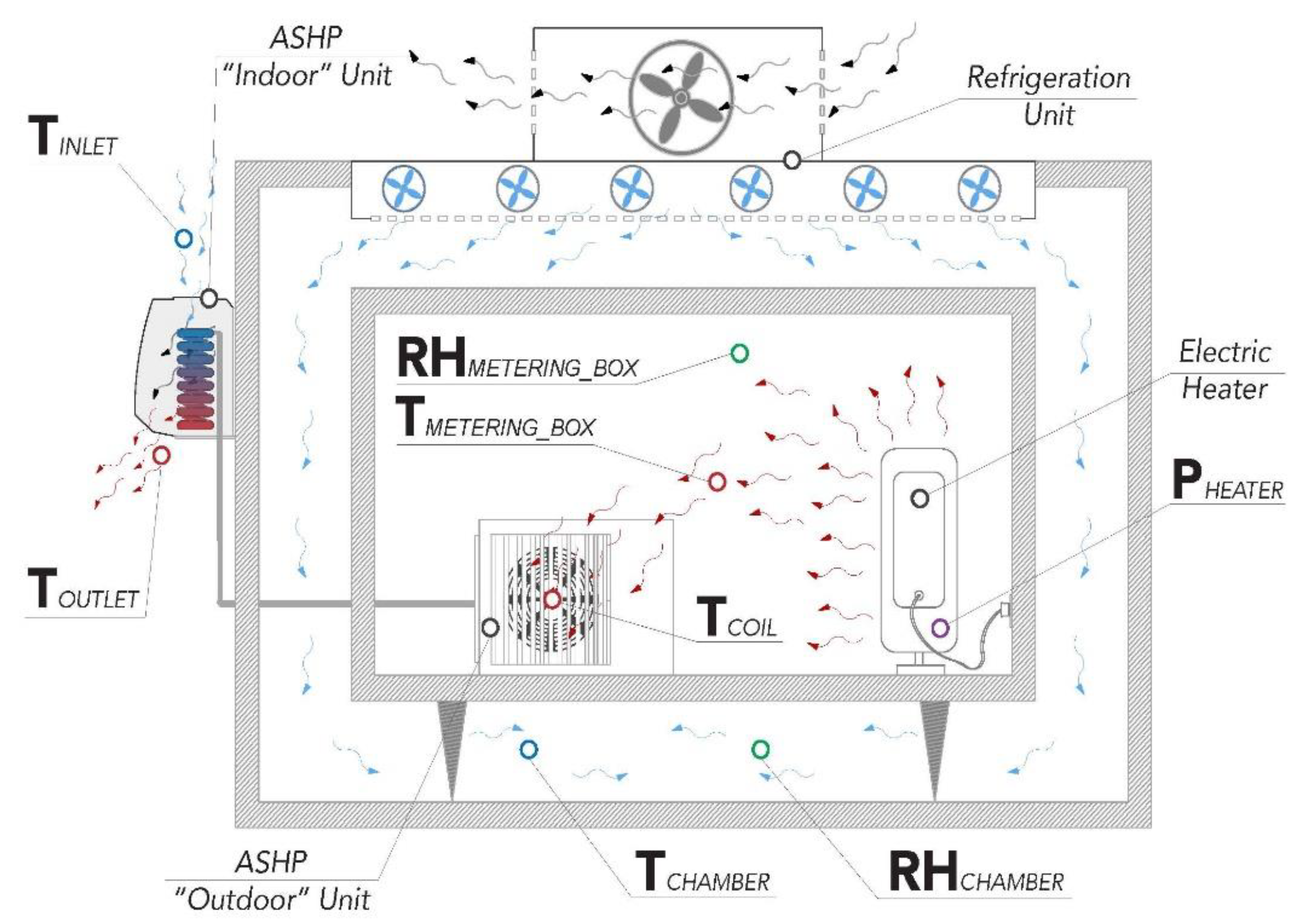
2.1. Measurement Method Overview

Four ductless mini-split ASHPs were evaluated in this study. Each heat pump was tested separately using a cold chamber. The temperature inside the chamber was controlled using its refrigeration system, and the heat load of the heat pump was controlled by adjusting the heat pump’s compressor speed (either directly or indirectly, as explained later). The temperature inside the chamber was varied from 10 °C down to −25 °C (except for one heat pump, which was only designed to operate down to −15 °C, and thus was only tested down to that temperature) in 5 °C intervals, and for each temperature, performance data were recorded at multiple heat loads.

The conceptual drawing of the experimental setup at the cold chamber is shown in Figure 1. As seen in the figure, there is a metering box (an insulated box) located inside the cold chamber, and the outdoor unit of the heat pump is installed inside this metering box. Inside the chamber, the temperature outside the metering box (T_CHAMBER) was set to a desired level and maintained using the refrigeration system, while the temperature inside the metering box (T_{METERING_BOX}) was controlled using an electric heater (which makes up for the heat removed by the heat pump) to maintain the temperature inside the metering box equal to the temperature outside the metering box. The fact that the temperature outside the metering box and inside the metering box was maintained equal means that there was no heat transfer occurring between those two spaces. It means that the heat removed by the heat pump was equal to the heat supplied by the electric heater, which was measured (P_HEATER). Thus, the purpose of the metering box was to allow for measuring the heat removed by the heat pump. The input electrical power of the ASHP was measured also (P_ASHP). The heat output of the ASHP was calculated from the physical law of energy conservation by adding the heat removed by the heat pump (determined from the heat supplied by the electric space heater) and the input electrical energy of the ASHP. The steady-state COP of the ASHP was calculated by dividing the heat output rate by the input electrical power of the ASHP after reaching a steady state. As shown in Figure 1, additional data were collected to gather information about the status of the heat pump’s operation and environmental conditions. For example, if the temperature of the ASHP outdoor unit’s heat exchanger (T_COIL) rises above the ambient temperature, it means that the heat pump is in a defrost mode that melts the ice accumulated on the heat exchanger. The indoor unit’s inlet temperature (T_INLET) and outlet temperature (T_OUTLET) were measured to help determine the status of the indoor unit. The relative humidity inside the chamber was measured inside the metering box (RH_{METERING_BOX}) as well as outside the metering box (RH_CHAMBER) to provide additional information about environmental conditions.

This cold chamber is located inside a large open high-bay lab, and the indoor unit of the ASHP was supplying heat into this open lab and reducing the amount of heat that was needed to be supplied by the lab’s main heating system (the experiment was performed during the heating season). The indoor temperature in the lab was maintained at around 21 °C.

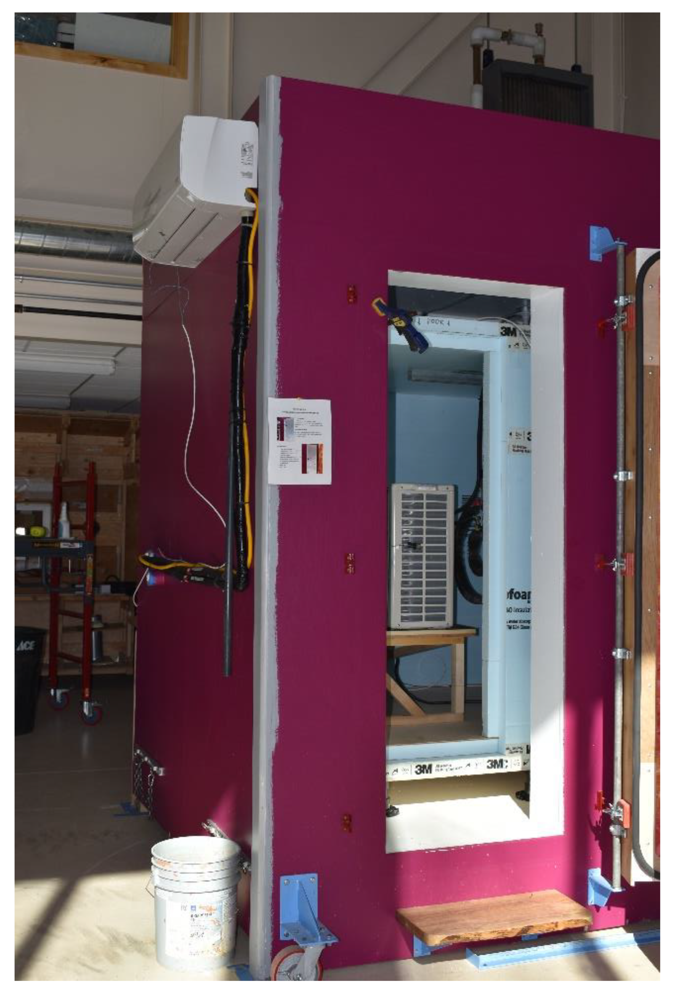
2.2. Cold Chamber Description

The cold chamber was custom built with a steel frame and approximately 18 cm (7 in.) of spray foam in the walls and floor. The freezer unit for the cold chamber, from Cincinnati Sub-Zero, sits on its roof and is sized to achieve temperatures down to −40 °C in the small enclosure. The cold chamber is designed to split apart in its middle, with one side on wheels resting on a track, so that equipment for different evaluations of building materials can be inserted inside, even if they are too large to fit through the man door, or for envelope materials to fit between the two sides for evaluation.

A metering box sits in the cold chamber interior. It is made of approximately 10 cm (4 in.) thick extruded polystyrene foam on all sides, with sheets of approximately 2 cm (¾ in.) thick plywood on the top and bottom of the floor. The size of the metering box represents a balance between allowing enough space for air flow around the metering box inside the cold chamber and allowing as much room as possible inside the metering box for the ASHP outdoor unit, to mimic the outdoor space in which it would typically be located. The interior dimensions of the cold chamber and metering box are shown in

Table 1. The dimensions of the cold chamber and interior metering box.

	Cold Chamber Interior	Metering Box Interior
Width	1.83 m (6 ft)	1.32 m (4.33 ft)
Length	2.91 m (9.56 ft)	2.23 m (7.33 ft)
Height	2.29 m (7.5 ft)	1.52 m (5 ft)

.

Figure 2 is a photograph of the cold chamber set up at the Cold Climate Housing Research Center (CCHRC) in Fairbanks, AK, USA, with a ductless ASHP installed. Visible through the man door of the cold chamber is the metering box made of blue extruded polystyrene foam, and inside that is the outdoor unit of the ASHP. The indoor unit of the ASHP is shown in the upper left, mounted on the cold chamber outside wall and connected to the outdoor unit by an electrical cable and refrigerant lines.

2.3. Instrumentation

The cold chamber and metering box setup contains a data monitoring system to collect the variables shown in the conceptual diagram of the experimental setup (Figure 1). Staff utilized a Campbell Scientific (Logan, UT, USA) data logging system, which consisted of a CR1000X datalogger and a PS150 12 V power supply with a battery backup. The datalogger was set to sample the data every second and convert it into 10-s, 1-min, and 5-min data for logging. The 1-min data were used for the analysis presented in this article.

To calculate the COP of the heat pump, researchers measured the power used by the heat pump and the power used by the electric heater in the metering box. In both cases, a Wattnode (Onset Computer Corporation, Bourne, MA, USA) T-WNB-3Y-208-P power meter [20] connected to two 30-amp current transformers (Magnelab (Longmont, CO, USA) SCT-0400-030) [21] was used.

Multiple temperature and relative humidity (RH) sensors were placed throughout the experimental setup and are listed with their purposes in

Table 2. Environmental sensors utilized and their purposes.

Sensor	Purpose
Temperature– Outdoor unit heat exchanger	To identify defrost cycles of the heat pump and serve as a check that other sensors are functioning properly.
Temperature and RH– Metering box	These sensors were placed inside the metering box and measured the “outdoor” temperature and relative humidity seen by the heat pump.
Temperature and RH– Chamber	These sensors were placed inside the cold chamber, but outside the metering box, to monitor respective environmental conditions.
Temperature– Indoor unit inlet	This measured the air temperature on the inlet of the indoor unit of the heat pump, which means the temperature of the “room” that the heat pump was heating.
Temperature– Indoor unit outlet	This was used to verify when the heat pump was providing space heating.

. The temperature sensors were thermistors from Littlefuse (Chicago, IL, USA) with model number PS103J2 [22]. The relative humidity sensors were from Honeywell (Charlotte, NC, USA), HIH-4000-002 [23].

2.4. Air Source Heat Pump Models and Controlling Their Thermal Output

The four ductless mini-split heat pumps used in this study and their relevant specifications are shown in

Table 3. Heat pump models used and their specifications.

Heat Pump Model	Outdoor Unit Model Number	Indoor Unit Model Number	Rated COP	Low Temperature Limit
Fujitsu RLS3H	AOU12RLS3H	ASU12RLS3Y	4.64	−26 °C
Daikin LV	RXS12LVJU	FTXS12LVJU	4.35	−15 °C
Panasonic ClimaPure XE	CU-XE12WKUA	CS-XE12WKUAW	4.39	−26 °C
Daikin Aurora	RXL15QMVJUA	FTX15NMVJU	4.0	−25 °C

. The specifications were taken from the manufacturers’ documentation [24,25,26,27].

Only built-in controls were utilized in this study, without purchasing any additional accessories (such as external thermostats). The intent was to record data for at least three different levels of thermal loading (which means three different compressor speeds) for each heat pump and each outdoor temperature (the term “outdoor temperature” herein is used for the temperature of the environment in which the outdoor unit of the ASHP is located, which in our study means the temperature inside the cold chamber). For each of the four heat pumps, the maximum compressor speed was achieved by setting the temperature setpoint to the maximum available value. Because the setpoint was significantly higher than the temperature in the lab (maintained around 21 °C), the thermostat was calling for the maximum heat output, which means the maximum compressor speed. Achieving other compressor speeds varied by the heat pump model as follows:

The Fujitsu (Tokyo, Japan) RLS3H heat pump has an “ECONOMY” mode as well as an “OUTDOOR UNIT LOW NOISE” mode available, both of which were used to achieve different levels of thermal output. In each of these two modes, the temperature setpoint was kept at the maximum available value. While the thermostat temperature setting was the same as when testing at the maximum compressor speed (explained above), the “ECONOMY” mode resulted in a significantly reduced thermal output, and the “OUTDOOR UNIT LOW NOISE” mode resulted in a thermal output that was significantly reduced even further.

The Daikin (Osaka, Japan) LV heat pump has an “ECONO” mode as well as an “OUTDOOR UNIT QUIET” mode available, both of which were used in a similar way as described above for the Fujitsu RLS3H heat pump. Unfortunately, the data collected in both of these modes resulted in very similar datapoints (in terms of the thermal output as well as COP). In order to avoid near duplication of the datapoints in the broader dataset used later for the analysis, the data collected in the “OUTDOOR UNIT QUIET” mode were discarded. As a result, only two levels of thermal loading (the maximum one and the one achieved in the “ECONO” mode) were available for this heat pump, even though the intent was to have at least three.

The Daikin Aurora heat pump has an “ECONO” mode available, but does not have a mode for the quiet operation of the outdoor unit. The “ECONO” mode was used in a similar way as described above. In order to achieve an additional level of thermal output, the thermostat temperature setting was lowered (in a normal mode, not in the “ECONO” mode) to a level just barely above a level that was causing the heat pump to turn off (which was determined through experimentation). This resulted in a low level of thermal output that was significantly below the one achieved in the “ECONO” mode, thus providing a third level of thermal output, as intended. However, unlike with previous settings, the electrical power input kept drifting (resulting in the thermal output drifting), and therefore, researchers kept adjusting the thermostat temperature setting throughout the experiment to compensate for the changes observed and keep the thermal output at near-constant levels.

The Panasonic (Osaka, Japan) ClimaPure XE heat pump has neither economy nor outdoor unit quiet modes available. Data were collected at two levels of thermal output using user-accessible settings–the maximum heat output (as described earlier) and a low heat output achieved by adjusting the temperature setpoint (in a similar way as described above for the Daikin Aurora heat pump). In order to collect data at additional levels of thermal output beyond what was possible with user-accessible settings, the heat pump’s test mode was utilized, which directly allows setting the compressor speed to predetermined levels. In the test mode, data were collected at the nominal, intermediate, and minimum compressor speeds. It means that altogether, data were collected at five different levels of thermal output for this heat pump.

2.5. Data Analysis Methodology

After turning on a heat pump and setting it as desired for the given test, the studied quantities start changing (for example, the input power starts climbing as the compressor speed starts ramping up), and it takes some time for them to reach a steady state. It is the steady-state data that is used for the analysis in this project. It means that for each heat pump, each outdoor temperature, and each thermal output studied, an attempt was made to continue the measurement until everything stabilized. It is the section of the time-series data where the studied variables are no longer changing (which means they reached a steady state and stay constant) that was utilized to capture the steady-state thermal output and COP. In some situations, the studied quantities kept fluctuating a little bit as opposed to reaching a constant value. However, as long as the central value of these fluctuations was no longer changing, it was considered a steady state, and the central value (average of the fluctuating quantity) was used for further analysis. There were situations when a defrost came before a steady state was reached. In those situations, the measurement continued to see if a steady state would be reached before the subsequent defrost (and if not, sometimes one more attempt was made). If a steady state was not reached in any of the attempts for the given settings, no datapoint was captured for those settings and thus was left out of the subsequent analysis.

Since the purpose of this research was not to study a specific heat pump model, but rather develop a more general understanding, the data for all heat pumps studied were combined into one dataset for the majority of the analysis in this project.

Because the maximum thermal output varied significantly among the individual heat pumps, the thermal output had to be normalized in order to combine the data for the individual heat pumps to study the impact of thermal loading on the COP. The maximum thermal output was found for each heat pump studied by taking the maximum thermal output found among all collected steady-state data points for the given heat pump (it is worth noting that for all heat pumps studied, this maximum thermal output occurred at 10 °C or 5 °C). The thermal output for each steady-state data point collected for each heat pump was expressed as a percentage of the maximum thermal output for that heat pump. This normalized thermal output is used for all analyses in this article, as opposed to the actual thermal output.

3. Results

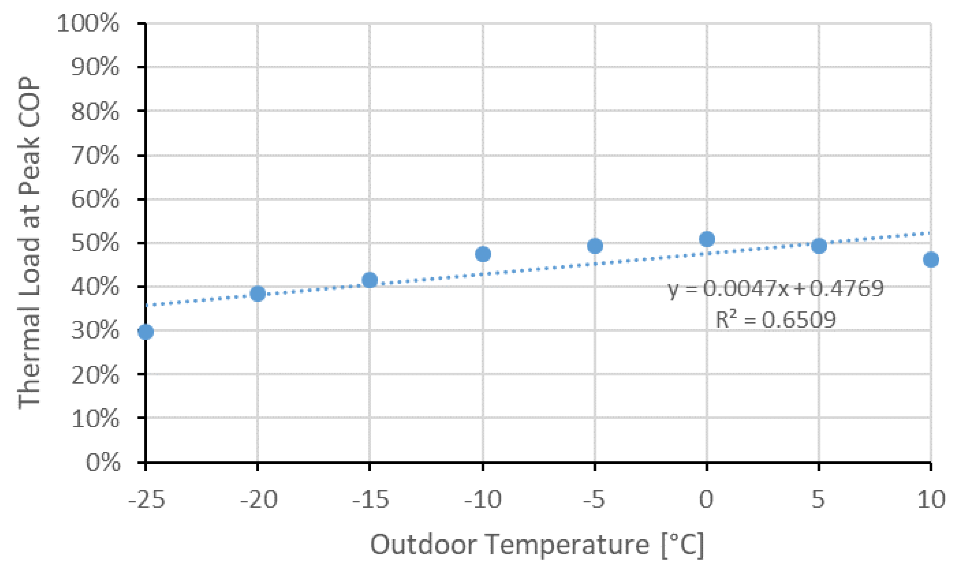
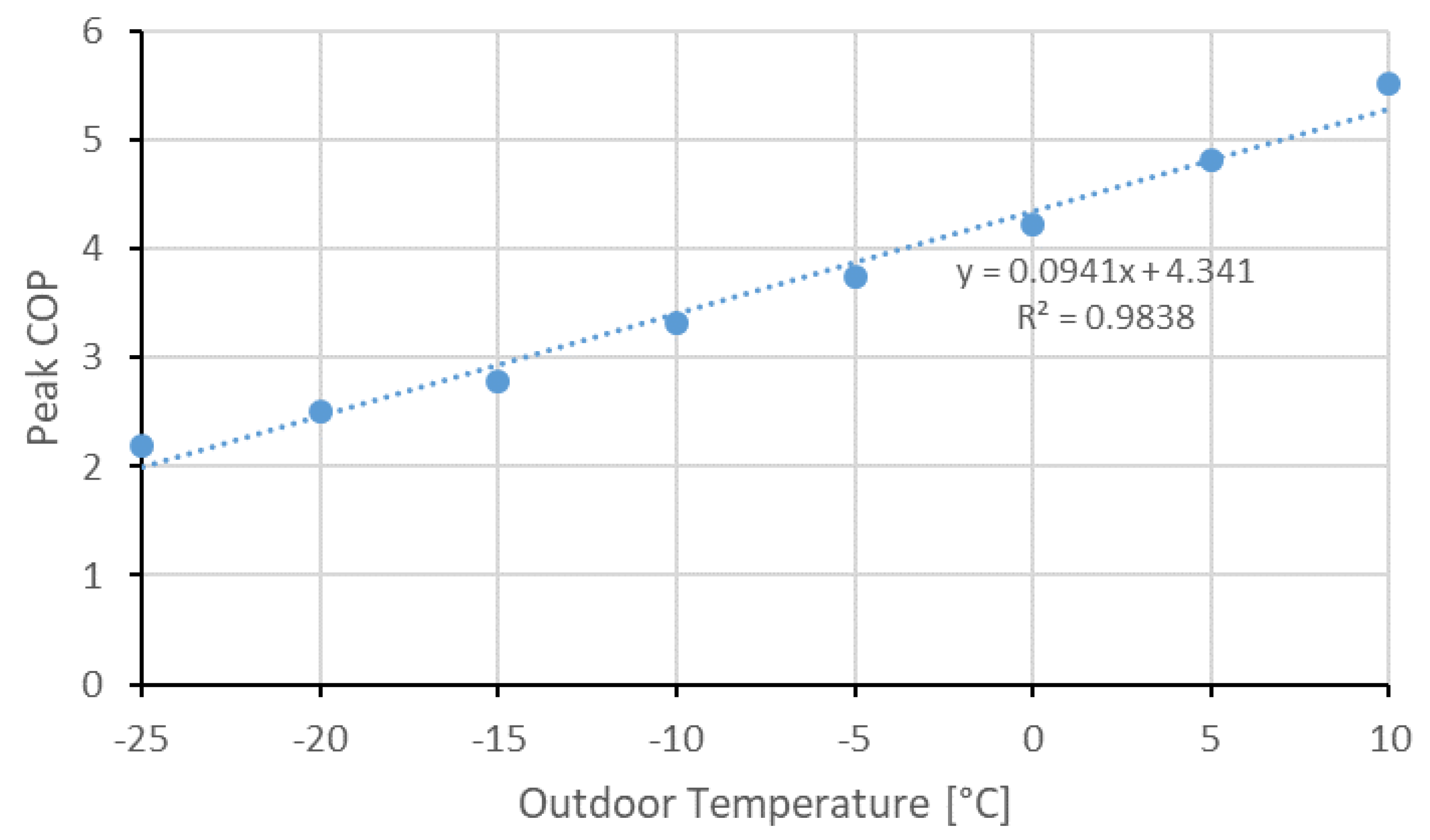
3.1. Experimental Data

Since the purpose of this research was not to study a specific heat pump model, but rather develop a more general understanding, the results presented herein represent data for all four studied heat pumps combined. Figure 3 shows the measured COP as a function of the outdoor temperature. Two series are presented in the graph. The first series shows the COP at maximum thermal loading. Because the COP peaks at levels of thermal loading that are below the maximum thermal loading (as shown further in the results), the second series shows the COP for the data points that were collected closest to the peak (which means the maximum COP measured).

As seen in Figure 3, the COP at maximum thermal loading was very similar for all heat pumps studied (as demonstrated by the very short whiskers), which made it possible to directly combine the COP values for all heat pumps studied for further analysis without having to normalize the COP values. This is unlike the maximum thermal output, which varied significantly among the individual heat pumps, and therefore had to be normalized (as explained earlier) before combining the steady-state data points for all heat pumps into a single dataset.

The steady-state COP for all heat pumps combined was plotted as a function of the normalized thermal output for each temperature studied. A second-order polynomial fit was added for each temperature. The resulting graph is shown in Figure 4.

As seen in Figure 4, the maximum achievable thermal output, in general, is lower for lower outdoor temperatures. While not the main focus of this study, this relationship was further investigated. For each outdoor temperature, the steady-state thermal output (normalized, as explained earlier) that was the highest one achieved at that temperature was taken for each heat pump studied and averaged into one value representing all heat pumps combined. This value was then plotted for each temperature, and the resulting graph is shown in Figure 5. This relationship will be useful for determining the upper limits of plots of the analytical function modeling the COP as a function of temperature and thermal loading in Section 3.2.

3.2. Analytical Function to Model COP as a Function of Temperature and Thermal Loading

In order to approximate the relationship shown in Figure 4 with an analytical function, it is important to further analyze that relationship. As seen in Figure 4, the COP as a function of thermal loading at a given outdoor temperature can be approximated with a second-order polynomial, which means a quadratic function. The peak of the curve occurs at different levels of thermal loading for different temperatures. This relationship is shown in Figure 6, and the values of the COP peaks for the different temperatures are shown in Figure 7.

Since the COP as a function of thermal loading can be approximated with a quadratic function, one can use a quadratic function as a starting point to create a model for the COP as a function of temperature and thermal loading. One of the forms of a quadratic function is the vertex form, which is known to be as follows:

y = a(x − h)² + k

(1)

where y is the dependent variable; x is the independent variable; and a, h, and k are the coefficients of the quadratic function in the vertex form. The dependent variable in our model is the COP of the heat pump, which means y in Equation (1) can be replaced with COP. Since the quadratic function is used to approximate the COP as a function of thermal load, x, as the independent variable, can be replaced with the thermal load. Thermal_load will be used as the designator for the thermal load, and since it represents the thermal load that is normalized (see Section 2.5), it can have values between 0 and 1 (which means between 0% and 100%). The a coefficient for the quadratic functions representing the trendlines in Figure 4 was somewhat different for different temperatures, and therefore it was averaged into a single value, with the result of a = –7.46. The h coefficient represents the x-coordinate of the peak of the quadratic function. The x-coordinate in our case is the thermal load, which means the h coefficient represents the thermal load at which the peak COP occurs. As shown in the graph in Figure 6, this thermal load depends on the outdoor temperature, and this dependence can be approximated with the linear function shown in the graph. Therefore, the h coefficient can be replaced with that linear function, resulting in h = 0.0047T + 0.477, where T is the outdoor temperature in °C. The k coefficient represents the y-coordinate of the peak of the quadratic function. The y-coordinate in our case is the COP, which means the k coefficient represents the peak COP. As shown in the graph in Figure 7, this peak COP depends on the outdoor temperature, and this dependence can be approximated with the linear function shown in the graph. Therefore, the k coefficient can be replaced with that linear function, resulting in k = 0.0941T + 4.34. After all these substitutions in Equation (1), the resulting expression is as follows:

COP = −7.46(Thermal_load − 0.0047T − 0.477)² + 0.0941T + 4.34

(2)

Equation (2) is the analytical function to model the steady-state COP as a function of the outdoor temperature and thermal loading. Plotting this analytical function results in a graph shown in Figure 8. The model was compared with the original data points collected (shown in Figure 4) and the coefficient of determination was calculated to be R² = 0.8911.

4. Discussion

As shown in Figure 3, for all heat pumps and temperatures studied, partial loading at a certain level resulted in an increased COP compared to maximum thermal loading (as indicated by the gap between the whiskers of the two series in the figure). This is expected, because the size of the heat exchangers stays the same, which means at a lower heat rate, the condensing and evaporating heat exchanger temperatures are closer to the heat sink and source temperatures, respectively, which yields a lower temperature lift and thus increases the COP. However, as seen in Figure 4, continuing to lower the thermal load eventually starts resulting in a declining COP. This can be due to the electrical power of the heat pump that is consumed by components other than the compressor (such as fans) becoming larger in its relative value compared to the heat output rate of the heat pump. This can also be due to the parasitic heat transfer within the heat pump (which when operating has warm and cold components/environments close to each other, thus resulting in heat transfer) becoming larger in its relative value compared to the heat output rate of the heat pump. It can also be that the compressor itself might operate with a lower efficiency at low speeds. Of course, it can be a combination of multiple effects, but verifying any of them or investigating their relative contributions was beyond the scope of this study.

It is generally understood that grossly oversizing heat pumps can lower the overall efficiency by increasing the proportion of the time when the heat pump cycles (to accommodate heat loads below the minimum compressor speed) [13]. However, knowing that the COP can decrease even before reaching the minimum compressor speed (as shown in Figure 4 and Figure 8) further underscores the potential risks of oversizing and emphasizes the complexity of the issue of sizing heat pumps. Ideally, a heat pump would be sized to always operate at its peak COP. Unfortunately, this is not possible because the heat load of a building increases with lower outdoor temperatures, while the optimum thermal output (the one that yields the highest COP) of a heat pump, in general, decreases with lower outdoor temperatures, as shown in Figure 6. The relationship between the COP, outside temperature, and thermal loading, as shown in this study, is such that no direct guidelines can be given for an optimal size of a heat pump and modeling needs to be used to determine what heat pump size yields the highest overall efficiency (or to determine the optimal balance between the initial cost and efficiency, but cost considerations were beyond the scope of this study). The analytical model presented in this article (see Equation (2)) can be used as a part of such modeling efforts. However, the model presented is a steady-state model and thus can be directly used only for steady-state scenarios. A typical heat pump installation will not always operate in a steady state and will experience some level of cycling. Cycling occurs when a heat pump operates below its minimum capacity, which is typically during periods of warmer weather (but still cold enough that some heating is needed). In this situation, the heat pump cycles by repeatedly turning on and off to accommodate the low heat load. Cycling also occurs during periods of cold weather when ice is building up on the outside heat exchanger. The heat pump needs to periodically defrost itself (typically by engaging a reversing valve and sending heat from the indoor unit to the outdoor unit) and thus operates in cycles. One recommendation for future research is to enhance the developed model by identifying conditions in which cycling occurs and applying a derate factor to the steady-state COP value returned by the model to account for the effects of the cycling.

Another recommendation for future research is to verify the applicability of the developed model to other heat pumps (as the model is based on four heat pumps only) and also investigate how the model can be used for heat pumps of other efficiencies. All four heat pumps in this study had a similar efficiency in terms of manufacturers’ specifications (and as shown in Figure 3, they also ended up having very similar COPs at maximum thermal loading). It is our hypothesis that the herein developed model (Equation (2)) could be used for heat pumps of other efficiencies by scaling the COP value up or down proportionally based on the manufacturer’s specifications for the efficiency of the given model. However, confirming this hypothesis was beyond the scope of this study.

As explained earlier, the purpose of this research was not to study a specific heat pump model, but rather develop a more general understanding of heat pump efficiency as a function of thermal loading at various outdoor temperatures. Therefore, the developed model is based on trendlines (which do not exactly match the data points for the individual heat pumps studied, but broadly represent the heat pumps as a group), seen in Figure 4. The developed analytical function expressing the COP as a function of outdoor temperature and level of thermal loading (plotted in Figure 8) approximates these trendlines, but does not exactly match them. Part of the reason is that this analytical function was meant to be simple enough to allow for its practical use. Because of that, some deviations exist between the analytical function (plotted in Figure 8) and the original trendlines (seen in Figure 4). For example, the biggest deviation in the peak COP occurs at the temperature of 10 °C, where the original trendline shows a peak COP of about 5.5 (see Figure 4), while the analytical function shows a peak COP of about 5.3 (see Figure 8), representing a deviation in the peak COP of about −4%. This deviation can also be seen in Figure 7 (by comparing the 10 °C data point to the linear trendline). The biggest deviation in the thermal load at which the peak COP occurs also happens to be at the temperature of 10 °C, where the original trendline shows that it occurs at the thermal load of about 46% (see Figure 4), while the analytical function shows that it occurs at the thermal load of about 52% (see Figure 8). This deviation can also be seen in Figure 6 (by comparing the 10 °C data point to the linear trendline).

The impact of thermal loading on a heat pump’s COP, as shown in this study, is such that no direct guidelines can be made with respect to using a temperature setback strategy. For example, if a heat pump operates at a thermal load that is close to its peak COP, the energy savings achieved by a temperature setback (for example at night, or during the day when occupants are away) might be outweighed by the extra energy use due to the lower COP at which the heat pump temporarily operates when coming back from the setback and operating at maximum thermal output. However, if a heat pump operates at a very low thermal load where the COP is low, for example, the COP at the full thermal output when the heat pump is coming back from the setback might not be significantly different (or it could even be higher, in some situations) and the setback strategy might achieve energy savings. These scenarios demonstrate that no direct guidelines can be made, and modeling needs to be used to determine whether there are net energy savings through a setback strategy in a given specific situation. The herein developed model can help in those efforts.

The relationship between thermal loading and COP shown in this study inspires potential innovative solutions to saving energy via utilizing heat pumps. For example, one solution to consider in cold climates is using two heat pumps where the second one would automatically turn on when it is cold outside and the first heat pump (when covering the full heating load) operates close to its maximum output and thus with a relatively low COP. Turning the second heat pump on would distribute the heat load among the two heat pumps (assuming proper controls) and potentially bring their thermal loading close to the point of the peak COP, thus saving energy. However, installing a second heat pump significantly increases the capital cost, so whether or not such a solution would make economic sense would have to be determined through modeling for the given specific situation.

5. Conclusions

In this study, the performance of four ductless mini-split heat pumps was evaluated in a lab to gain a broader understanding of the relationship between the COP, outside temperature, and thermal loading. An empirical model of this relationship was created. To make the use of the model practical in building energy simulations, it was approximated with a relatively simple analytical function (Equation (2)) that expresses the steady-state COP as a function of the outside temperature and thermal loading. The model represented by the analytical function was found to be in reasonable agreement (R² = 0.8911) with the original data collected.

The plot of the COP as a function of thermal load for different temperatures (Figure 8) shows that it is difficult to create direct guidelines for sizing and operating heat pumps for maximum efficiency and modeling needs to be used to determine optimal choices in specific situations.

It should be noted that there are other factors that affect heat pump efficiency besides the outdoor temperature and level of thermal loading. Examples of such factors are fan speeds or the ceiling clearance of the indoor unit of a ductless mini-split system. It is our recommendation for future studies to evaluate such factors in order to further guide the deployment of heat pumps and maximize their benefits.

The empirical model developed in this study advances the ability to make optimal choices with respect to sizing and operating air source heat pumps and contributes to saving energy and increasing the sustainability of energy practices in our society.

References

1. Energy Consumption by Source, World. Available online: https://ourworldindata.org/grapher/energy-consumption-by-source-and-region (accessed on 26 July 2022).
2. Ristinen, R.; Kraushaar, J.; Brack, J. Energy and the Environment, 3rd ed.; Wiley: Hoboken, NJ, USA, 2016. [Google Scholar]
3. Air-Source Heat Pumps. Available online: https://www.energy.gov/energysaver/air-source-heat-pumps (accessed on 26 July 2022).
4. Marsik, T.; Stevens, V. Air Source Heat Pumps in Cold/Arctic Climates. In Proceedings of the Thermal Systems in Cold/Arctic Climates Forum, Fairbanks, AK, USA, 21–24 January 2020. [Google Scholar]
5. Northeast Energy Efficiency Partnerships. Cold Climate Air-Source Heat Pump Specification (Version 3.1); Northeast Energy Efficiency Partnerships: Boston, MA, USA, 2021; Available online: https://neep.org/sites/default/files/media-files/cold_climate_air-source_heat_pump_specification-version_3.1_update_.pdf (accessed on 26 July 2022).
6. Northeast Energy Efficiency Partnerships. Northeast/Mid-Atlantic Air-Source Heat Pump Market Strategies Report 2016 Update; Northeast Energy Efficiency Partnerships: Boston, MA, USA, 2017; Available online: https://neep.org/sites/default/files/NEEP_ASHP_2016MTStrategy_Report_FINAL.pdf (accessed on 26 July 2022).
7. Caskey, S.; Kultgen, D.; Groll, E.; Hutzel, W.; Menzi, T. Simulation of an Air-Source Heat Pump with Two-Stage Compression and Economizing for Cold Climates. In Proceedings of the International Refrigeration and Air Conditioning Conference, West Lafayette, IN, USA, 16–19 July 2012; Available online: http://docs.lib.purdue.edu/iracc/1278 (accessed on 31 July 2022).
8. RDH Building Science Inc. BC Cold Climate Heat Pump Field Study; RDH Building Science Inc.: Victoria, BC, Canada, 2021; Available online: https://www.rdh.com/wp-content/uploads/2021/01/BC-Cold-Climate-Heat-Pump-Study-Final-Report.pdf (accessed on 26 July 2022).
9. Winkler, J. Laboratory Test Report for Fujitsu 12RLS and Mitsubishi FE12NA Mini-Split Heat Pumps; National Renewable Energy Laboratory: Golden, CO, USA, 2011. Available online: https://www.nrel.gov/docs/fy11osti/52175.pdf (accessed on 31 July 2022).
10. Williamson, J.; Aldrich, R. Field Performance of Inverter-Driven Heat Pumps in Cold Climates; Consortium for Advanced Residential Buildings, Steven Winter Associates, Inc.: Norwalk, CT, USA, 2015. Available online: https://www.nrel.gov/docs/fy15osti/63913.pdf (accessed on 30 July 2022).
11. Pollard, A.; Berg, B. Heat Pump Performance, BRANZ Study Report SR414; BRANZ, Ltd.: Judgeford, New Zealand, 2018; Available online: https://www.researchgate.net/publication/330717027_Heat_pump_performance (accessed on 30 July 2022).
12. U.S. Environmental Protection Agency. ENERGY STAR Program Requirements, Product Specification for Smart Thermostat Products, Eligibility Criteria, Draft 1 Version 2.0; U.S. Environmental Protection Agency: Washington, DC, USA, 2022. Available online: https://www.energystar.gov/sites/default/files/asset/document/ENERGY%20STAR%20Version%202.0%20%20Smart%20Thermostat%20Draft%201%20Program%20Requirements.pdf (accessed on 30 July 2022).
13. Northeast Energy Efficiency Partnerships. Guide to Sizing & Selecting Air-Source Heat Pumps in Cold Climates; Northeast Energy Efficiency Partnerships: Boston, MA, USA, 2018; Available online: https://neep.org/sites/default/files/resources/ASHP%20Sizing%20%26%20Selecting%20-%208x11_edits.pdf (accessed on 31 July 2022).
14. Northeast Energy Efficiency Partnerships. User Guide: Cold Climate Heat Pump Sizing Support Tools; Northeast Energy Efficiency Partnerships: Boston, MA, USA, 2022; Available online: https://ashp-production.s3.amazonaws.com/NEEP_ccASHP+Heating+Visualization+User+Guide_v2.2_TRC_04.01.22.pdf (accessed on 31 July 2022).
15. CanmetENERGY. Air-Source Heat Pump Sizing and Selection Guide; Natural Resources Canada: Ottawa, ON, Canada, 2020. Available online: https://www.nrcan.gc.ca/sites/nrcan/files/canmetenergy/pdf/ASHP%20Sizing%20and%20Selection%20Guide%20(EN).pdf (accessed on 31 July 2022).
16. Torregrosa-Jaime, B.; Martínez, P.J.; González, B.; Payá-Ballester, G. Modelling of a Variable Refrigerant Flow System in EnergyPlus for Building Energy Simulation in an Open Building Information Modelling Environment. Energies 2019, 12, 22. [Google Scholar] [CrossRef] [Green Version]
17. Smith, I. Variable Speed Heat Pump Product Assessment and Analysis; Northwest Energy Efficiency Alliance: Portland, OR, USA, 2022; Available online: https://neea.org/resources/variable-speed-heat-pump-product-assessment-and-analysis (accessed on 31 July 2022).
18. Bagarella, G.; Lazzarin, R.; Noro, M. Sizing strategy of on–off and modulating heat pump systems based on annual energy analysis. Int. J. Refrig. 2016, 65, 183–193. [Google Scholar] [CrossRef]
19. Cold Climate Air Source Heat Pump Product List. Available online: https://ashp.neep.org/ (accessed on 31 July 2022).
20. Wattnode T-WNB-3Y-208-P Data Sheet. Available online: https://www.testequipmentdepot.com/onset/pdf/twnb3y208p_datasheet.pdf (accessed on 3 December 2022).
21. Magnelab SCT-0400 Series Spec Sheet. Available online: https://www.magnelab.com/wp-content/uploads/2015/02/SCT-0400-Spec-Sheet.pdf (accessed on 3 December 2022).
22. Littlefuse PS Series Data Sheet. Available online: https://m.littelfuse.com/~/media/electronics/datasheets/leaded_thermistors/littelfuse_leaded_thermistors_interchangeable_thermistors_standard_precision_ps_datasheet.pdf.pdf (accessed on 3 December 2022).
23. Honeywell HIH-4000 Series Product Sheet. Available online: https://prod-edam.honeywell.com/content/dam/honeywell-edam/sps/siot/en-us/products/sensors/humidity-with-temperature-sensors/hih-4000-series/documents/sps-siot-hih4000-series-product-sheet-009017-5-en-ciid-49922.pdf (accessed on 3 December 2022).
24. Fujitsu 12RLS3H Submittal Data. Available online: https://www.fujitsugeneral.com/us/resources/pdf/support/downloads/submittal-sheets/12RLS3H.pdf (accessed on 2 October 2022).
25. Daikin FTXS12LVJU/RXS12LVJU Submittal Data. Available online: https://backend.daikincomfort.com/docs/default-source/product-documents/residential/submittal/ftxs12lvju-rxs12lvju.pdf (accessed on 2 October 2022).
26. Panasonic CS-XE12WKUAW/CU-XE12WKUA Submittal Data. Available online: https://panasonic.ca/brochures/EN/housing/heating-ac/CS-XE12WKUAW_Submittal_Ver3.0_en.pdf (accessed on 2 October 2022).
27. Daikin FTX15NMVJU/RXL15QMVJUA Submittal Data. Available online: https://backend.daikincomfort.com/docs/default-source/product-documents/residential/submittal/ftx15nmvju-rxl15qmvjua-submittal.pdf (accessed on 2 October 2022).
Figure 1. Conceptual drawing of the cold chamber, metering box inside the cold chamber, and the experiment setup for heat pump performance measurements.
Sustainability 15 01880 g001
Figure 2. The cold chamber and metering box set up for evaluating ductless ASHPs in the CCHRC laboratory space.
Sustainability 15 01880 g002
Figure 3. Steady-state COP as a function of the outdoor temperature for all heat pumps combined. Markers represent average values (the COPs of the individual heat pumps averaged into one value), while whiskers represent minimum and maximum values (the COPs of the worst- and best-performing heat pump in the given conditions).
Sustainability 15 01880 g003
Figure 4. Steady-state COP as a function of thermal load for all heat pumps combined. For each studied outdoor temperature, the graph shows the data points collected as well as a second-order polynomial trendline.
Sustainability 15 01880 g004
Figure 5. The highest achievable steady-state thermal output (average of all heat pumps) as a function of the outdoor temperature. The graph also includes a second-order polynomial trendline.
Sustainability 15 01880 g005
Figure 6. The thermal load (normalized per procedure described earlier) at which the peak COP occurs as a function of the outdoor temperature. The graph also includes a linear trendline, the equation for that trendline, and the coefficient of determination (R2).
Sustainability 15 01880 g006
Figure 7. The peak COP (which means the peaks of the second-order polynomial trendlines in Figure 4) as a function of the outdoor temperature. The graph also includes a linear trendline, the equation for that trendline, and the coefficient of determination (R2).
Sustainability 15 01880 g007
Figure 8. Plot of the analytical function that models the steady-state COP as a function of the thermal load and outdoor temperature.
Sustainability 15 01880 g008