Article

Electrification of Last-Mile Delivery: A Fleet Management Approach with a Sustainability Perspective

Department of Industrial Engineering, Universidad Nebrija, Calle Santa Cruz de Marcenado 27, 28015 Madrid, Spain
*
Author to whom correspondence should be addressed.
Sustainability 2023, 15(24), 16909; https://doi.org/10.3390/su152416909
Submission received: 24 October 2023 / Revised: 5 December 2023 / Accepted: 14 December 2023 / Published: 16 December 2023
(This article belongs to the Section Air, Climate Change and Sustainability)

Abstract

:
Light commercial vehicles that operate in last-mile deliveries are significant contributors to greenhouse gas emissions. For this reason, carbon footprint mitigation actions have become a key issue for companies involved in urban freight transport to put the organization in line with the future EU legislative framework. In this sense, the electrification of the delivery fleets is one of the actions carried out to improve the sustainability of transport operations. To this end, fleet managers have to explore several fleet renewal strategies over a finite planning horizon, evaluating different types of electric powertrains for light commercial vehicles. To address this concern, this paper presents a purpose-built analysis to assist and boost the fleet managers’ decisions when transitioning to electrified vans, intending to maximize cost savings and reduce corporate greenhouse gas emissions inventory. The model developed for this research work is a Multi-Objective Linear Programming analysis for the optimization of the total cost of ownership and the organizational transport-related emissions reported from all scope categories according to the Greenhouse Gas Protocol standards. This analysis is applied to three types of electric vans (battery electric, hydrogen fuel cell, and range extender hybrid electric/hydrogen fuel cell), and they are compared with an internal combustion van propelled with natural gas. From this perspective, the conducted research offers a novel approximation to fleet replacement problems considering organization emission reporting and long-term budgetary objectives for vehicles and their respective refueling infrastructure. The comprehensive numerical simulations carried out over different study scenarios in Spain demonstrate that the optimization approach not only shows effective fleet renewal strategies but also identifies critical factors that impact the fleet’s competitiveness, offering valuable insights for fleet managers and policymakers. The findings indicate that in Spain, battery electric and hydrogen range extender light commercial vehicles stand as a competitive option. Substituting a natural gas-powered van with an electrified alternative can reduce an organization’s inventory emissions by up to 77% and total costs by up to 24%. Additionally, this study also points out the influence of energy supply pathways and the emissions from relevant scope 3 categories.

1. Introduction

All European Union (EU) Member States are working toward achieving climate neutrality by 2050. In pursuit of this objective, the European Green Deal introduces a collection of measures outlining the EU’s approach to achieving this goal. Within these initiatives, the road transport sector plays an important role. According to the European Environment Agency (EEA), by 2019, greenhouse gas emissions from road transport have risen by 28% from 1990 levels, whereas the EU has witnessed a substantial reduction of 24% in its overall emissions [1]. Within this sector, light commercial vehicle (LCV) emissions stand out with a contribution of almost 12% and marking a substantial 63% increase compared with the growth rates observed in passenger cars and heavy-duty vehicles [2]. From a legislative point of view, the European Commission has recently proposed improvements in the actual Energy Taxation Directive (ETD) [3] in addition to the current EU legislative framework that includes pricing instruments based on CO2 emissions for road transport emissions [4].
Furthermore, the European Commission has set a goal to achieve carbon dioxide-free urban logistics in EU city centers by the year 2030 [5]. Last-mile transport activities represent a significant weight in the cities’ greenhouse emissions (GHG), largely owing to the dense populace and concentrated economic endeavors that characterize these regions [6]. In the city of Madrid, for example, in 2019, 38% of total traffic volume was due to the urban transport of goods, and it is expected to grow up to 47% in 2025 [7].
Within this context, many Spanish transportation companies have fixed a goal of zero-emission balance by 2050 [8] without losing sight of economic aspects because last-mile delivery operations are responsible for up to 41% of the total cost of the supply chain [9]. Therefore, the objectives pursued are improving cost savings and reducing the organizational carbon footprint according to the company’s environmental commitment [10,11]. Accordingly, one of the most important measures is to prioritize the adoption of electric vehicles, and thus, van fleet renewal is becoming a key factor in the fleet management strategy [12]. Moreover, these measures can additionally contribute to enhancing the company’s financial outcomes and bolstering its reputation [13]. Nevertheless, the path to fleet electrification is complex, entailing numerous decisions, ranging from the selection of vehicles and energy supply infrastructure to the management of operations [14].
In the literature, the use of electric vehicles for urban delivery activities heavily relies on their cost effectiveness and understandably reduced GHG emissions during their operation. To address the expense calculation, fleet operators consider the total discounted cost of ownership (TDCO) as the determining factor. Typically, TDCO methodology integrates the present value of all the vehicle costs to accurately assess the actual expenses of employing a specific vehicle alternative [15]. On the other hand, for the evaluation of the vehicle’s environmental performance, the methodologies applied utilized some of the basic phases in the lifecycle analysis (LCA). LCA is often referred to as a “cradle-to-grave” assessment and analyzes the emissions along the stages of the vehicle’s life, from extracting and processing raw materials to its final disposal or recycling at the end of its lifespan [16,17,18,19]. It is essential to highlight that TCO and LCA results depend on the location where the vehicles are operating [20,21]. Nevertheless, there are scarce research works that have analyzed the uptake of electric LCVs for last-mile activities in fleet replacement problems, simultaneously considering cost and emissions issues [22,23,24].
However, none of these previous studies have taken into account the integrated information derived from the interaction between economic data and non-financial information expressed through the annual sustainability company report in a commitment to Corporate Social Responsibility (CSR). This information is essential for fleet management [25,26]. Additionally, most of the preceding research dismisses the energy supply infrastructure investments for using electrified vans in actual commercial fleets, but it is an important fact due to the limited availability of high-capacity public recharging points and the virtual absence of urban hydrogen refueling stations (HRS) [27].
This holistic approach is the key to making appropriate fleet replacement decisions and is one of the main contributions of this research work. To this end, the authors have developed a Multi-Objective Linear Programming (MOLP) analysis to efficiently explore viable fleet renewal strategies. The objectives are both the optimization of the total cost of ownership and the organizational transport-related emissions reported from all scope categories according to the Greenhouse Gas Protocol standards [28]. Considering organizational boundaries, the competitiveness of different types of electric powertrains for light commercial vehicles, such as battery electric (BEV), hydrogen fuel cell (FCEV), and hydrogen fuel cell range extender (FCEREV), was evaluated. Afterward, these electric options are compared with an internal combustion van propelled by natural gas (CNG).
The comprehensive numerical simulations carried out over different study scenarios in Spain demonstrate that the optimization approach not only shows effective fleet renewal strategies but also identifies critical factors that impact the fleet’s competitiveness. Additionally, the optimized fleet mix is compared with a fleet composed only of CNG vans. In this sense, the fleet operator managers could analyze the effect of tailored model fleet parameters, such as the van purchase price, van ownership period, the annual mileage demand, and the emissions intensity of the energy for van fueling. The investigation approach considers the particular characteristics of electric LCVs, the corporate emissions boundaries, and the on-site van energy supply pathway. Furthermore, to assess the strength of the optimized strategies and provide valuable insights into the model parameter relationships, a robustness scenario analysis and a descriptive statistical correlation matrix were conducted.
The main contributions of this research can be outlined as follows:
  • A comprehensive optimization approach by integrating MOLP and Greenhouse Gas Protocol standards for corporate emissions accounting and reporting;
  • Optimization of the fleet mix and minimizing cost and emissions accounted for in the corporate sustainability report throughout the entire service life of the vehicle in the fleet;
  • Assessing cost and emissions issues simultaneously for different types of electric powertrains for LCVs, considering their on-site refueling infrastructure means;
  • Assessment of the energy supply pathway used. The electricity mix and the use of hydrogen purchased or on-site produced by electrolysis have been taken into account. In the case of purchased hydrogen, it is explored the use of blended green hydrogen with 40% of hydrogen obtained via steam methane reforming (SMR);
  • Highlighting the weight of scope 3 emissions in the corporate sustainability report for last-mile transport activities using electrified vehicles in the fleet.
From this perspective, the developed analysis framework makes it possible for fleet operators to improve the van replacement decision-making process according to corporate policy.
This paper is organized as follows: The Section 2 focuses on fleet replacement problems with GHG emissions considerations in previous investigations. The methodology and materials are in the following section, explaining the optimization model, the economic and environmental evaluation, the scenario definition, and the data used in the investigation. Section 4 shows the results and their interpretation. Finally, conclusions are placed in the foreground.

2. The Literature Background

In fleet management, a critical concern of fleet renewal problems is determining the optimal timing and type of vehicles for replacement. Contrary to earlier research studies that concentrated on fleet optimization models for reducing long-term expenses [29], the optimization model outlined in this study places its emphasis on reaching the optimal fleet mix and minimizing cost and emissions accounted for in the corporate sustainability report throughout the entire service life of the vehicle.
Despite some research investigations that explore the environmental and economic effectiveness of using electric vehicles [30,31,32], there is scarce literature that has investigated strategies for vehicle replacement considering GHG emission reduction and economic viability simultaneously. Table 1 summarizes the research studies analyzed and how the authors’ research study fits within the existing literature. Most of the optimization methods utilized for fleet renewal management challenges relied on a linear programming (LP) model. Moreover, the optimization problem is expressed in single (SO) or multiple (MO) objective functions, taking into account specific country market characteristics. However, for SO approximation, it is not possible to achieve a balance between economic and environmental objectives, and the optimal solution is highly dependent on the economic magnitude of the vehicle ownership costs. Moreover, the models are subjected to certain constraints, considering that the fleet has an adequate number of vehicles to fulfill transportation requirements and satisfy a budget limit.
The research studies considered have used the TDCO approach for the economic evaluation. Moreover, the environmental impact is evaluated through the GHG emissions converted to a cost function using a carbon tax. However, the research works differ in the scope of cost and emissions quantification. In the case of the total cost of ownership, the studies consider the vehicle acquisition and operating costs but dismiss the on-site energy supply infrastructure for electric vans. Concerning emission quantification, some of the studies expand the vehicle emissions during operation and incorporate emissions associated with some of the basic phases in the LCA of a product defined by ISO 14040:2006 [37], such as manufacturing, operation, maintenance, and disposal, and some investigations include emissions associated with the extraction of raw materials, fuel production, or manufacture and installation of the necessary energy supply infrastructure. Nevertheless, all the studies analyzed sum up all the emissions, and none of them consider the corporate emissions reporting scopes (scopes 1, 2, and 3) for assessing and quantifying sources of emissions. Additionally, BEVs receive full attention while fuel cell vehicles are dismissed.
Therefore, the developed MOLP analysis allows for efficient exploration of viable fleet renewal strategies over a defined planning horizon. The objectives are the optimization of the total cost of ownership and the organizational transport-related emissions reported from all scope categories according to the Greenhouse Gas Protocol standards. Considering organizational boundaries, it assessed, at the same time, the competitiveness of different types of electric powertrains, taking into account the vehicle and energy supply infrastructure costs and focusing on the scopes of the emissions computed in the corporate emissions report. In this light, the conducted research offers a novel approximation to fleet replacement problems, enabling a breakdown analysis for costs and emission scopes.

3. Materials and Methods

The multi-objective linear replacement optimization model is based on two cost-objective functions to be minimized, the total cost of ownership and the corporate carbon footprint focused on transport activities at the organizational level. Quantifying a company’s carbon footprint involves measuring its direct and indirect GHG emissions expressed in units of CO2 equivalent weight (kg CO2e). Figure 1 shows the approach used to fix the problem of optimal van fleet renewal.
Objective functions are combined using the weighted sum method, forming one aggregate objective function (AOF); hence, the initial MO problem has been changed into an SO optimization problem. This approach is the simplest and most widely used to solve MO engineering problems [38].
Afterward, comprehensive optimizations were performed over different study scenarios in Spain. Additionally, the long-term optimized fleet mix is compared with a fleet composed only of CNG vans. In this sense, the fleet operator managers could analyze the effect of tailored fleet operator requirements, such as the annual mileage demand, the van ownership period, fleet size, the corporate emission report scopes, and the on-site van energy supply pathway.
Finally, to reduce the model parameters uncertainty, a sensitivity scenario analysis of the critical fleet factors was conducted. Furthermore, to assess the strength of the optimized strategies, a robustness analysis was conducted.
For every particular solution, the model outcome comprises the fleet composition in each year of the planning horizon (number of vans and energy supply infrastructure assets in use, purchased or retired), a set of economic results (the cost per kilometer and the cost breakdown), and environmental results (the emissions per kilometer and the emissions breakdown per scope).
This section has been split into three parts. The initial subsection is focused on establishing the model and providing the mathematical framework for the linear optimization algorithm. Afterward, the scenario settings executed by the optimization algorithm are exposed. Finally, the model input data are outlined and described.

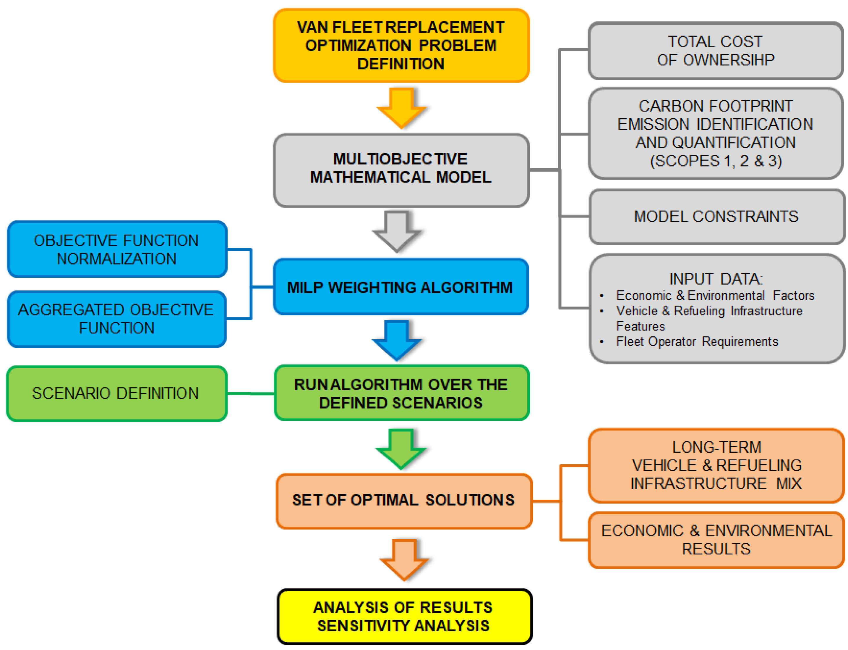
3.1. Model Definition and Mathematical Formulation

The model developed for the optimization of the fleet renewal challenge relies on deterministic linear programming. Moreover, it is considered that the fleet size is enough to meet transport demand, but there is a budget limit.
The mathematical expression of the optimization problem is based on the algorithm developed by Figliozzi [33]. The novelty relies on the consideration of the refueling infrastructure costs and the incorporation of the corporate carbon footprint quantification objective function split in scopes. Thus, the original SO changed to an MO optimization problem. For a better understanding, the model indices, parameters, and decision variables are explained in Table 2, Table 3 and Table 4.
The mathematical expression of the MO algorithm is shown in Equation (1). The objective function is a weighted combination of the economic aspects ( f E C O ) calculated using the TDCO method and the expected monetary burdens for carbon emissions ( f E N V ). Since the objective functions have different scales, it is necessary to standardize them into a non-dimensional format. This process is commonly known as normalization.
M i n i m i z e :     w 1   f E C O Z E C O m a x + w 2 f E N V Z E N V m a x  
where
w 1 ,   w 2 are the weighting coefficients, where s w s = 1 , and 0   w s   1 ;
Z E C O m a x     represents the scalarization factor for the objective function f E C O . It is computed as the highest value of the f E C O N within the context of the examined current scenario.
Z E N V m a x     represents the scalarization factor for the objective function f E N V . It is computed as the highest value of the f E N V within the context of the examined current scenario.
In this approach, the weights ( w s ) represent the fleet operator’s pre-established preferences. To find an approximation of the Pareto frontier, the optimization algorithm varies the weighting coefficients from 0 to 1 and solves successive problems. Nevertheless, the appropriate choice of these weights can prove to be a considerable challenge. For this purpose, the authors have used the method proposed by Shahriari [39] to find the suitable weights, as explained in Equation (2).
w 1 o = β 1 β 1 + β 2   w 2 o = 1 w 1 o
where
β 1 = Z E C O * ( Z E C O Z E N V * ) 2 ;   β 2 = Z E N V * ( Z E N V Z E C O * ) 2 ;
Z E C O * is the evaluation of the objective function f E C O at its optimal solution X E C O * , and it is defined as
Z E C O * = f E C O ( X E C O * )
Z E C O   is the evaluation of the objective function f E C O at the optimal solution of the objective function f E N V ( X E N V * ), and it is defined as Z E C O = f E C O ( X E N V * ) .
Z E N V * is the evaluation of the objective function f E N V at its optimal solution X E N V * , and it is defined as
Z E N V * = f E N V ( X E N V * )
Z E N V   is the evaluation of the objective function f E N V at the optimal solution of the objective function f E C O ( X E C O * ), and it is defined as Z E N V = f E N V ( X E C O * ) .
In this sense, it is possible to highlight three key solutions over the Pareto frontier (Figure 2): economic (ECON— X E C O * ); environmental (ENV— X E N V * ); and balanced (BAL– X B A L * ). The ECON solution provides the highest cost reductions ( w 1 = 1 ) , but the ENV solution shows the highest emission savings ( w 2 = 1 ) . However, the BAL solution is calculated considering the highest emissions savings are achieved with the lowest cost increase ( w 1 = w 1 * , and w 2 = 1 w 1 * ). The w 1 * value is obtained iteratively from w 1 o   until a predefined percentage for cost reduction is achieved.
The aggregated cost-objective function defined in Equation (1) is governed by the constraints expressed in Equations (3)–(30). Every year, the fleet vans have to travel the distance specified by the fleet operator (Equation (3)). Equations (4) and (5) ensure that the quantity of acquired type “k” vans aligns with the new registrations of type “k” van entries. Equation (6) determines that the initial number of type “k” vans is calculated by the sum of vans of type “k” in operation and vans disposed of by the conclusion of the initial period. Equation (7) ensures the balance of van numbers year-on-year. Each van must be disposed of by the end of the final year (Equation (8)). Upon the completion of its ownership period, a van is obligated to be disposed of (Equation (9)), and a newer van cannot be sold until it reaches the ownership period (Equations (10) and (11)). Equations (12) and (13) dictate the substitution of aging vehicles with new counterparts. There is a yearly budget limit for purchasing new vans (Equation (14)). Equations (15) and (16) express that there are sufficient charging points to recharge every day all the electric vans in the fleet, while the HRS must possess the capability to refuel the entire fleet of hydrogen-powered vans stationed at the depot daily (Equations (17) and (18)). Whenever hydrogen vans are present, there should be a minimum of one dispenser accessible (Equation (19)). Equation (20) indicates an annual budget for acquiring new energy supply infrastructure assets. The number of newly purchased infrastructures of type “r” must match the infrastructures of type “r” in use each year (Equations (21) and (22)). The energy supply infrastructure assets are in operation throughout the entire analysis period (Equations (23) and (24)). The energy supply infrastructure assets should be decommissioned when reaching their service life (Equation (25)) or the last year of the planning horizon (Equation (26)). Infrastructures can not be scratched before reaching their service life (Equations (27) and (28)). Equations (29) and (30) show that variables are integer or binary numbers.
i = 0 N k 1 k = 1 K v X i j k · U i j k N y · d j       j     { 0 ,   1 ,   2 ,   ,   T 1 }  
P 00 k + X 0 0 k = X 00 k         k  
P 0 j k X 0 j k = 0       k     j     (   1 ,   ,   T )  
X i 0 k + S i 0 k = X 0 i k       k     i     ( 1 ,   ,   N k )
X ( i 1 ) ( j 1 ) k = X i j k + S i j k       k     j     ( 1 ,   ,   T )     i     ( 1 ,   ,   N k )
X i T k = 0       k     i     ( 0 ,   1 ,   N k 1 )
X N k j k = 0       k     j     ( 1 ,   ,   T )
S 0 j k = 0       k     j     ( 0 ,   ,   T 1 )
S i 0 k = 0     k       i     ( 0 ,   ,   N k )
X i j k R · Y i j k       k     j     ( 1 ,   ,   T 1 )   i     ( 0 ,   ,   N k )
n = 0 i 1 S n j k R · ( 1 Y i j k )     k       j < T       i < N k
k = 1 k v P 1 j k · V P C k j P V b j     j     ( 0 ,   ,   T 1 )
i = 0 N 2 1 X i j 2 N S I 1 · m = 0 M 1 1 I X m j 1       j     ( 0 ,   ,   T 1 )
i = 0 N 2 1 X i j 2 + i = 0 N 3 1 X i j 3 N S I 1 · m = 0 M 1 1 I X m j 1 + N S I 2 · m = 0 M 2 1 I X m j 2     j     { 0 ,   1 ,   2 ,   ,   T 1 }
i = 0 N 4 1 X i j 4 N S I 4 · m = 0 M 4 1 I X m j 4     j     ( 0 ,   ,   T 1 )
i = 0 N 3 1 X i j 3 N S I 3 · m = 0 M 3 1 I X m j 3 + N S I 4 · m = 0 M 4 1 I X m j 4     j     ( 0 ,   ,   T 1 )  
i = 0 N 3 1 X i j 3 + i = 0 N 4 1 X i j 4 N S I 5 m = 0 M 5 1 I X m j 5       j     ( 0 ,   ,   T 1 )
r = 1 R i I P 1 j k · I P C k j P I b j       j     ( 0 ,   ,   T 1 )
I P 00 r + I X 0 0 r = I X 00 r         r
I P 0 j r I X 0 j r = 0       r     j     (   1 ,   ,   T )
I S m 0 r + I X m 0 r = I X 0 m r       r     m     (   1 ,   ,   M r )
I X ( m 1 ) ( j 1 ) r = I X m j r + I S m j r       r     j     ( 1 ,   ,   T )     m     ( 1 ,   ,   M r )
I X m T r = 0       r     m     ( 0 ,   ,   M r 1 )
I X M r j r = 0       r     j     ( 1 ,   ,   T )
I S m j r = 0       r     j     ( 0 ,   ,   T 1 )       m     ( 0 ,   ,   M r 1 )
I S 0 T r = 0         r
X i j k , S i j k ,   P j k ,   I X m j r ,   I S m j r ,   I P j r     Z  
Y i j k     { 0 ,   1 }

3.1.1. Total cost of ownership calculation

TDCO encompasses the complete ownership expenses of the asset, whether it is a vehicle or infrastructure, computed annually. The total cost of ownership is expressed in present value terms, incorporating adjustments for discount rates and inflation. The cumulative yearly expenditures of the fleet are established through the aggregation of vehicle costs and the associated refueling infrastructure, as expressed in Equation (31). Among the latter, variable costs include energy and maintenance and repair (M&R) expenses, while fixed costs cover circulation taxes and fees for insurance. Concerning infrastructure costs, the acquisition and scrapping values and M&R costs are considered.
f E C O = A P V V R V + V O P + A P I I S V + I O P
where
APV is the vehicle acquisition cost, defined as
A P V = j = 0 T 1 k = 1 K v A P V j k · V A j k · ( 1 + r i f ) j ( 1 + r d ) j
VRV is the revenue due to the vehicle resale at the end of the ownership period. It is defined as
V R V = j = 0 T i = 1 N k k = 1 K v A P V ( j i ) k · V D R i k · V S i j k · ( 1 + r i f ) j ( 1 + r d ) j
VOP is the vehicle operating cost (fixed and variable) due to the energy consumed, M&R activities, circulation taxes, and fees for insurance. It is defined as
V O P = j = 0 T 1 i = 0 N k 1 k = 1 K v [ ( V E C i j k + M C V i j k + R C V i j k ) · D i j k + F C i j k ] · V O i j k · ( 1 + r i f ) j ( 1 + r d ) j
API refers to the acquisition cost of energy supply infrastructure. It is defined as
A P I = j = 0 T 1 r = 1 R i A P I j r · I A j r · ( 1 + r i f ) j ( 1 + r d ) j
ISV represents the revenue attributed to the residual value of the infrastructure upon completion of the service life. It is defined as
I S V = j = 0 T m = 0 M r r = 1 R i A P I j r · I S R m r · I S m j r · ( 1 + r i f ) j ( 1 + r d ) j
IOP is the infrastructure operating cost due to the M&R activities, defined as
I O P = j = 0 T 1 m = 0 M r 1 r = 1 R i ( M C I m j r + R C I m j r ) · I O m j r · ( 1 + r i f ) j ( 1 + r d ) j

3.1.2. Evaluation of Corporate Carbon Footprint

To assess the carbon footprint, the authors have taken into account the guidelines outlined by the GHG Protocol [28] because it is one of the most widely used tools for assessing emissions inventories in companies [40]. The first step for corporate carbon footprint quantification is to delimit the scope of emissions according to organizational boundaries, followed by the emissions inventory data collection. In this research, the organizational boundaries are specified under the operational control approach, and in this case, it is focused on transport activities. Hence, the calculation of the corporate footprint considers GHG emissions derived from (i) transport realized by the company’s vehicles (scopes 1 and 2), (ii) cradle-to-gate emissions stemming from the company’s acquisition of fuels and energy, and the corresponding transport and distribution losses of purchased electricity (scope 3—3rd category), and finally, (iii) cradle-to-gate emissions of the vehicles purchased by the company (scope 3—2nd category). In addition, this investigation considers the energy supply facilities acquired to fulfill van operational requirements. In this sense, these assets are in the 1st category of scope 3. Nevertheless, in this study, due to the power magnitude of the infrastructure means and the long lifetime considered, it is supposed that the emissions intensity of the acquired energy supply components is negligible compared to the emissions due to electricity production considered in scope 2 [41,42,43]. Furthermore, the investigation scope considers on-road operation emissions from energy consumption; therefore, maintenance and repairing related emissions are overlooked. The cost-objective function for the carbon footprint quantification ( f E N V ) is displayed in Equation (32).
f E N V = E Q S 1 + E Q S 2 + δ S C · E Q S 3
where
EQS1 is the quantification of the emissions included in scope 1. It is defined as
E Q S 1 = j = 0 T 1 i = 0 N k 1 E Q 1 C N G · V O i j 1 · C E P j · ( 1 + r i f ) j ( 1 + r d ) j
EQS2 is the quantification of the emissions included in scope 2. It is defined as
E Q S 2 = j = 0 T 1 i = 0 N k 1 k = 1 K v E Q 2 E V k · V O i j k · C E P j · ( 1 + r i f ) j ( 1 + r d ) j
The variable δ S C is binary, assuming a value of one when scope 3 emissions are taken into consideration.
EQS3 quantifies the emissions encompassed within scope 3. It is defined as
E Q S 3 = j = 0 T 1 i = 0 N k 1 k = 1 K v δ S C · [ ( E Q 3 V A N k · V A j k ) + ( E Q 3 H 2 k · V O i j k ) ] · C E P j · ( 1 + r i f ) j ( 1 + r d ) j
The calculations used for the GHG accounting in each scope are explained in the following subsections. Additionally, for the quantification of GHG emissions, an emission factor (EF) [44] measured in kg CO2e is used.

Direct Emissions: Scope 1

This category accounts for emissions arising from the fuel usage of the company’s van fleet. Equation (33) quantifies the GHG emissions based on the yearly van CNG consumption.
E Q 1 C N G = E C N G · E F C N G
where:
E F C N G   is the EF associated with CNG

Indirect Emissions: Scope 2

This category comprises emissions linked to the purchased electricity utilized for van operations. In this study, there are three sources of electricity consumption depending on the type of electric van:
  • BEV: the electricity power consumption comes from recharging the battery;
  • FCEREV: the electric power consumption is derived from both battery and hydrogen supply;
  • FCEV: the electricity is used for hydrogen supply.
The electricity consumption for hydrogen supply depends on the hydrogen pathway used. In the case of purchasing hydrogen in 20 MPa pressurized tanks, the electricity consumption comes from raising the pressure to 90 MPa and pre-cooling before dispensing the hydrogen into the vehicle. Conversely, for on-site hydrogen production by electrolysis, it is necessary to add the electrolyzer and the compressor consumption to raise the pressure from the electrolyzer outlet to 90 MPa. Equation (34) expresses the emission quantification based on the yearly electricity consumption.
E Q 2 E V k = E e k · E F e
where
E F e   is the EF associated with the Spanish electricity production mix

Other Indirect Emissions: Scope 3

This category encompasses emissions attributed to van manufacturing as well as those related to the value chain of the energy consumed.
The indirect GHG emission electricity included in this scope comes from transmission losses of the purchased electricity reported in scope 2. Equation (35) calculates the emissions based on the yearly electricity consumption and a grid loss factor (GLF). The GLF quantifies the grid losses and depends on the transmission distance. Usually, the GLF can be rated from 3 to 14% of the energy transmitted [45]. A 6% value is used in this study according to the International Energy Agency’s recommendations [46].
E Q 3 E V k = G L F · E e k · E F e
Furthermore, in the case of hydrogen purchased, the emissions from hydrogen production, conditioning, and distribution are considered. If hydrogen production uses renewable energy sources, it is counted as zero emissions. The distribution mode considered employs trailers with diesel trucks. The trailer hydrogen mass transportation capacity ( Q H 2 ) is 700 kg at 20 MPa [47] per trailer with a distance separating the hydrogen generation location and the end-user ( D H 2 )   at most of 300 km. The energy spent in the compression of hydrogen is between adiabatic and isothermal ideal-gas compression values, and it is considered an electricity consumption for hydrogen pressurization of up to 20 MPa ( E e P H 2 ) of 1.8 kWh/kg [48]. The EF associated with hydrogen pressurization and truck transportation is calculated in Equation (36). The evaluation of this expression results in 1.2 kg/CO2e per kg of hydrogen transported; this value is more conservative than others used in related studies [41,49], which consider less than 1 kg/CO2e.
E F H 2 T = ( E e P H 2 · E F e ) + ( D H 2 · C F t r u c k · E F d i e s e l ) Q H 2  
where:
C F t r u c k = 0.345   L / km is the truck fuel consumption;
E F d i e s e l   is the EF considered for diesel
Equation (37) expresses the emission quantification based on a yearly van hydrogen consumption. Although in this research work, the main concern is the utilization of hydrogen derived from sustainable sources, for sensitivity analysis purposes, the scenario where the hydrogen supplied to fuel the fleet is blended with 40% of hydrogen obtained via steam methane reforming (SMR) is considered. These emissions are allocated in scope 3—1st category.
E Q 3 H 2 k = E H 2 k · ( E F H 2 T + p · E F H 2 _ S M R )
where
E F H 2 T is the EF calculated according to Equation (36);
E F H 2 _ S M R   is the EF associated with SMR hydrogen
p is the percentage of blended hydrogen.
The emission associated with the acquisition of vans is assigned to scope 3—2nd category and calculated according to Equation (38). In this scope, the emissions related to the manufacturing stage are considered, not contemplating the end-of-life emissions because the vans will be sold in the second-hand market. For the manufacturing emission analysis, a simplified vehicle model has been designed, which is composed of a body and an engine unit and includes not only the vehicle’s manufacturing emissions but also the exploitation of raw materials [50]. It is supposed that the EF associated with van body manufacturing is the same for all the van types analyzed. However, this is not the case for the engine unit, which is different for each technology.
E Q 3 V A N k = ( M V B k · E F V B ) + i ( P W k , i · E F k , i )  
where
M V B k is the k-type van body mass
E F V B are the cradle-to-gate GHG emissions related to vehicle chassis manufacture
P W k , i is the ith powertrain component characteristic of the k-type van: electric motor; traction battery; fuel cell system; hydrogen tank; CNG tank; and ICE powertrain
E F k , i are the cradle-to-gate GHG emissions associated with the ith powertrain component

3.2. Definition of Scenarios

A scenario reflects a probable situation of the vehicle fleet in the Spanish market [51]. The design of the scenarios revolves around three key fleet operator variables, two emission reporting modes (with or without scope 3 emissions), and two hydrogen supply pathways. The fleet operator variables are the yearly distance to be covered by each van in the fleet, the van ownership period, and the size of the fleet. In the same way, the supply pathway for the hydrogen refueling station (HRS) located at the depot could be acquired from a supplier (P scenarios) or generated on-site using an electrolyzer (G scenarios). Table 5 summarizes the variable values for the different scenarios. The baseline scenario is configured according to the business-as-usual behavior of Spanish fleets.

3.3. Model Data

The significant assumptions that depict the operation of last-mile delivery vehicles, as employed in this study, are outlined below:
  • The planning horizon time frame is 25 years (2025 to 2050);
  • At the beginning of the planning horizon, the fleet company has a specific quantity of CNG vans evenly distributed across various ages, spanning from 0 to the duration of the ownership period, and there are no energy supply infrastructures for electric vans;
  • The budgetary limit for acquiring vehicles and infrastructure assets is high enough to facilitate the replacement of older vans with the highest-cost electric van.
Data for cost objective function ( f E C O ), such as initial fleet conditions, fleet manager requirements, van and energy supply infrastructure technical features, and the economic parameters are compiled from Castillo [51]. Table 6 compiles the basic economic parameters needed for the optimization simulations.
Furthermore, the compilation of environmental data for the economic quantification of the carbon footprint ( f E N V ) has uncertainty due to the diversity of data sources, collecting methodologies, and locations considered, but it is representative of the European area. Table 7 compiles the GHG EF for the carbon footprint quantification referred to as van energy consumption. Additionally, Table 8 and Table 9 show the van powertrain characteristics and the respective GHG EF needed for the evaluation of the emissions accounted for in scope 3 related to vehicle manufacturing.
Finally, the carbon pricing forecast for the complete planning horizon is based on the data shown in the Carbon Pricing Dashboard of The World Bank [61]. In this report, the carbon pricing in Spain is EUR 18/tonCO2e, and the maximum value reached in Sweden is EUR 137/tonCO2e. The average value is EUR 77.5/tonCO2e, and it is used as the reference for this investigation.

4. Results and Discussion

The optimization algorithm is executed over the scenarios described in the preceding paragraph. In each scenario, the ECON, ENV, and BAL solutions from the Pareto frontier have been selected. However, the BAL solution ensures a balance between the competing objectives of cost savings and emission reductions, and it will be considered the optimal solution for further discussion in this section. Furthermore, the selected solutions are compared with a reference solution, where the van considered for replacing the old one is always the CNG type.
The optimization algorithm provides a set of results that comprises the following:
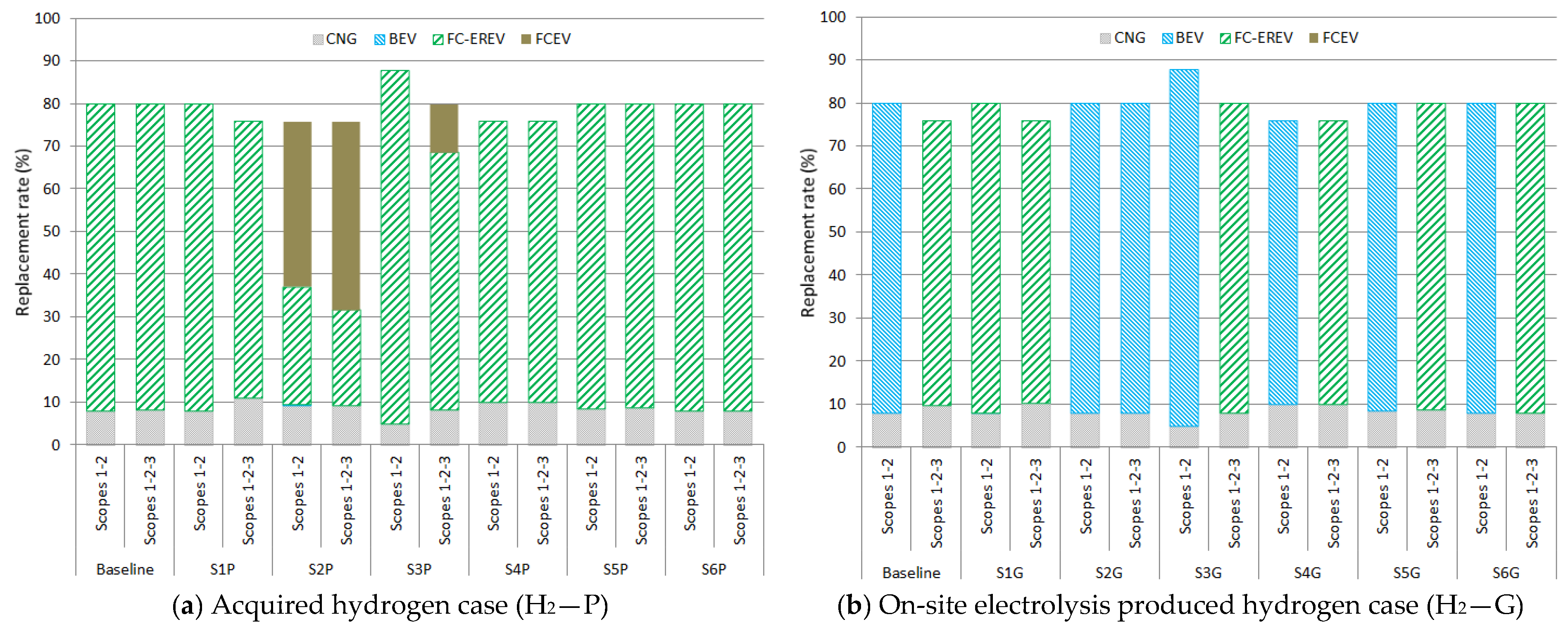
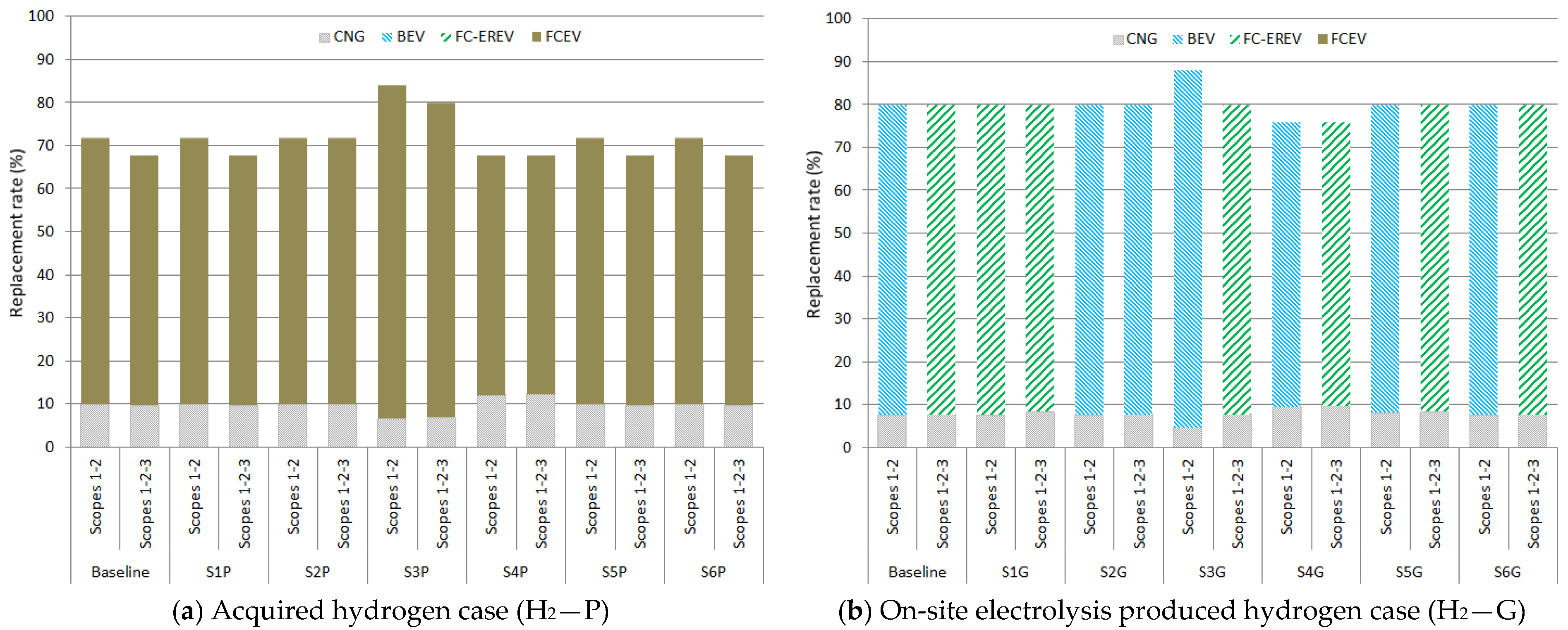
  • Fleet mix: distribution of fleet vehicles (type and age) every year within the planning horizon and the evolution of the infrastructure required to service the van fleet. These results are post-processed and translated into the fleet share and the replacement rate parameters. The fleet share shows the average share of each type of electric van in the fleet, and the replacement rate expresses the percentage of time when the electric vans in the fleet are the majority (over 90%);
  • Economic results: average cost per kilometer of the fleet and cost breakdown;
  • Environmental results: average emissions per kilometer of the fleet and emissions broken down into scopes 1, 2, and 3.
Finally, for the baseline scenario and BAL solution, a sensitivity analysis over different combinations of the model parameters to calibrate their effect on the fleet mix, cost, and emissions rate per kilometer is conducted. The sensitivity is evaluated with the expression shown in Equation (39).
E ( E s , X v s ) = Δ E s E s ¯ Δ X v s X v s ¯
where
Es is the emissions or cost rate per kilometer in the scenario “s”;
Xvs is the model parameter “v” in the scenario “s”.
Afterward, the robustness of the solutions is evaluated using the worst-case scenario analysis. The outcomes derived from the sensitivity assessment make it possible to fix the key parameters used to build up the worst-case scenarios.

4.1. Fleet Mix

Figure 3, Figure 4 and Figure 5 show the fleet share and the replacement rate for ECON, ENV, and BAL solutions in all the scenarios analyzed. Concerning fleet mix, the FCEREV van is the type of van most frequently used for the BAL and ECON solutions in H2P scenarios (Figure 3a and Figure 4a), regardless of the emission reporting scope. However, the FCEV van is the best option for the ENV solution (Figure 5a). This type of van also has a chance in the BAL solution for higher annual mileage (S2-P) and shorter ownership periods with scope 3 emission reporting (S3-P) (Figure 3a) for the lower impact of green hydrogen production, distribution, and conditioning compared to the electricity production mix and transmission losses. On the other hand, in the H2G scenarios (Figure 3b, Figure 4b and Figure 5b), the selected van types are BEV and FCEREV, depending on the scenario parameters and emission reporting scopes. The selected van type is FCEREV in all the scenarios for the BAL and ENV solutions when scope 3 emissions are accounted for (Figure 3b and Figure 5b), except in the scenario with higher annual distances traveled (S2-G), where BEV is the best option. These results are due to the higher manufacturing emissions of BEV vans compared to FCEREV counterparts but the higher emissions in on-site hydrogen production. The FCEREV van is also selected in low annual mileage scenarios (S1-G); it benefits from low hydrogen consumption due to the electric autonomy and the lower consumption.
As shown in Figure 3a,b, for BAL solutions, the EV replacement rate depends mainly on the ownership period, the van purchase price, and the emissions of scope 3 accounting. As expected, the replacement rate is lower in longer ownership periods (scenarios S4-P and S4-G). Additionally, the higher purchase cost of FCEV vans limits the replacement rate in the scenarios where they are used (S2-P, S3-P, and S4-P). Finally, if scope 3 emissions are taken into account, especially in H2P scenarios, the EV replacement rate is lower. The latest fact is due to the reduction in the difference in the emissions level between CNG and electrified vans. This effect is especially noteworthy in scenarios with lower mileage (S1-P) and shorter ownership periods (S3-P), where the operation emissions caused by the use of CNG vans do not affect considerably, and the effect of manufacturing emissions of electrified vans has relevance.

4.2. Economic and Environmental Results

Figure 6 shows the emission breakdown per scope and the average cost and emissions per kilometer for the BAL solution in each of the scenarios analyzed. As can be observed, the average emissions and costs per kilometer depend mainly on the yearly mileage, the van ownership period, and the scopes included in the company emissions report. In particular, the emissions are higher in H2G scenarios except for those with the lowest annual mileage (S1-P and S1-G), where H2P and H2G show similar emission levels. On average, the difference is 20.7% when the emissions scopes reported are 1 and 2 and 16% if scope 3 emissions are considered.
The highest average emission level for H2P scenarios (Figure 6a) with FCEREV vans is reached in the S1-P scenario regardless of the emissions scopes considered, with a high share of CNG vans in the fleet. Nevertheless, when scope 3 emissions are accounted for, the average emissions reached in short ownership periods (S3-P) is high.
However, in H2G scenarios, the maximum value of emissions is reached with the longest ownership period (S4-G) and BEV vans when only scopes 1 and 2 are considered (Figure 6b) due to the high presence of CNG vans in the fleet. But when scope 3 emissions are considered, the maximum is obtained in the opposite scenario, with the shortest ownership period (S3-G) and FCEREV vans. This finding points out the importance of scope 2 emissions due to the on-site hydrogen production using electricity from the grid. It is interesting to note that the S1-G scenario (Figure 6b) achieves a low level of emissions using FCEREV vans in the fleet.
With respect to the average costs per kilometer, considering an average price for hydrogen and electricity of EUR 4.2/kg and EUR 168/MWh, respectively, the H2P and H2G scenarios, regardless of emission scopes, show a similar cost level except for the H2P scenario with higher annual mileages (S2-P) (Figure 6a). In this scenario, there exists a noteworthy presence of FCEV vans in the mix, and the cost is significantly higher. Regarding H2P scenarios, the lowest cost per kilometer is reached with FCEREV vans in cases with moderate annual mileages (30.000 km) and longer ownership periods (S4-P). However, in the H2G case, there are BEV vans with the largest annual distance (S2-G) in this scenario. Additionally, shorter ownership periods (S3-P and S3-G scenarios) lead to higher costs per kilometer than longer periods (S4-P and S4-G scenarios). As expected, these results point out the higher acquisition costs of electric vans in comparison to CNG vans. Finally, the fleet size has a significant cost effect in scenarios where there are fuel cell vans. In this sense, in small fleets, the cost is higher.
Concerning the distribution of emissions per scope, it should be pointed out the following aspects:
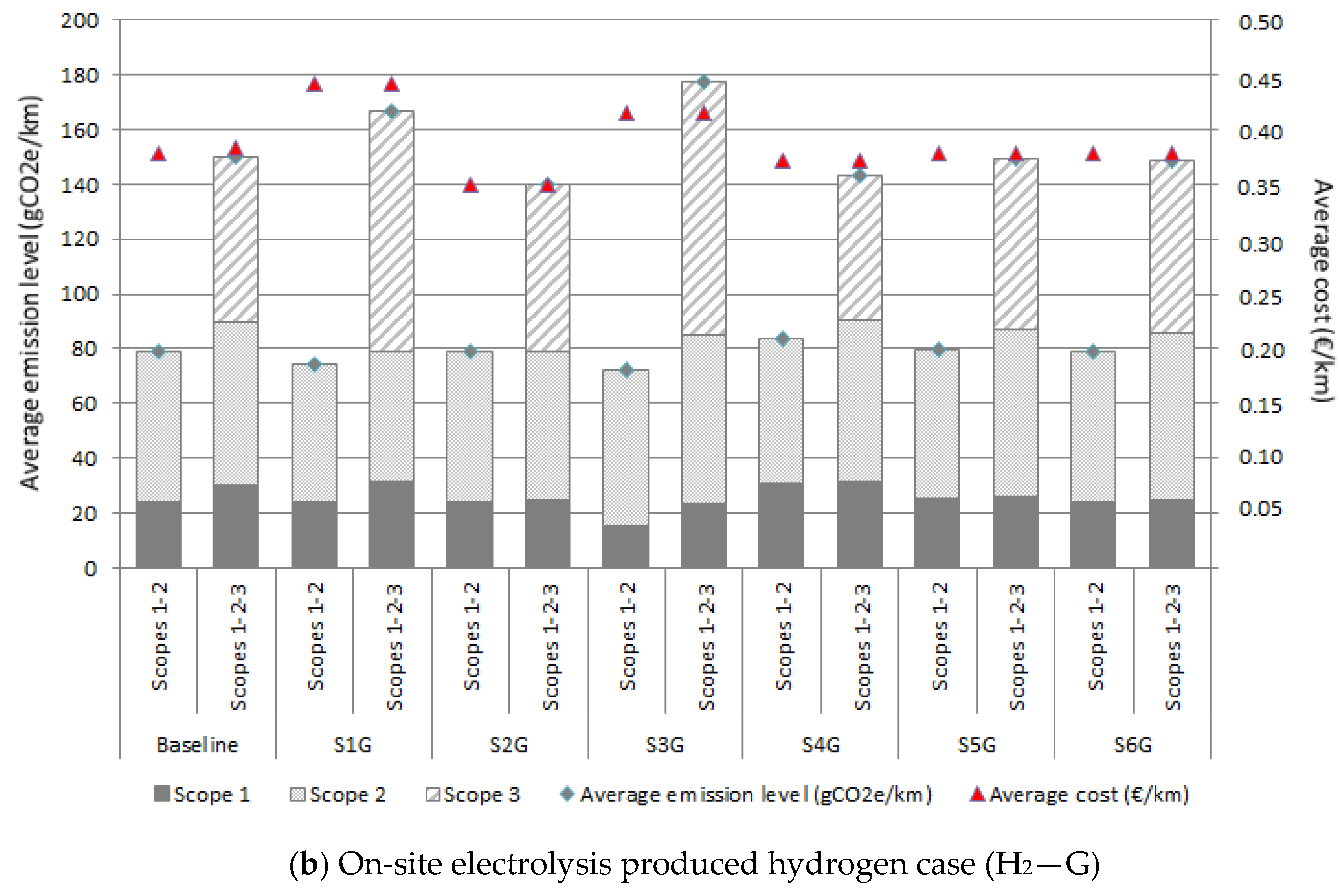
  • The consideration of scope 3 in the emissions report increases the level of accounted emissions average of over 71% in H2P and H2G scenarios;
  • The emissions reported in scope 3 have approximately the same weight as the sum of the emissions accounted for in scopes 1 and 2, except for the S4 scenarios with the longest ownership period. Additionally, when emissions in scope 3 are considered, the emission level in scope 1 grows. This is a result of the increased presence of CNG vans in the fleet mix;
  • The emissions reported in scope 2 are always higher in H2G scenarios than in the H2P. The major and minor differences are shown in the S2 and S1 scenarios, with the largest and lowest annual mileages, respectively. However, the emissions in scope 3 are higher in H2P scenarios except for the scenario with the higher annual mileage (S2). These results highlight the importance of the electricity production mix and the hydrogen distribution in scenarios with high distances traveled per year;
  • Concerning van selection, the consideration of scope 3 emissions has a low effect in H2P scenarios with FCEREV and FCEV vans in the fleet mix. Nevertheless, accounting for scope 3 emissions in H2G scenarios changes the preferred van option from BEV to FC-EREV, except for the longest annual mileage (S2-G).
On the other hand, the results obtained suggest an increment in costs when there is an emission cutback. Figure 7 reflects the emission savings and cost increase for the BAL solutions compared to the ECON solutions on a standardized 0–1 scale. In general, the cost increase mainly depends on the energy supply pathway and van type selected for the optimal solution.

4.3. Sensitivity and Solution Robustness Analysis

The results obtained for the BAL solutions in the baseline scenario are summarized in Table 10 for H2P scenarios and Table 11 for H2G scenarios. The fleet size change is excluded from the tables because it has no significant effect. The results show that the optimization solutions are sensitive to the electricity EF, the yearly mileage, and the van ownership period, followed by the purchase price of fuel-cell-powered vans and the discount rate and inflation, whereas the fuel-cell-powered van maintenance cost and the electricity price show a lower effect. Concerning related hydrogen parameters, only H2P scenarios are affected. The hydrogen price has a high influence in scenarios with higher yearly mileages, over 30.000 km. Nevertheless, the EF of blended hydrogen has a low effect.
Additionally, from this analysis, it can be observed that modifying model parameters does not result in a shift in the selected van type except for H2P scenarios with a high reduction in the electricity EF and higher annual mileages with scope 3 emissions reporting. The reduction in electricity EF means that several types of electric vans can participate in the fleet mix, while higher annual mileage opens up the opportunity for the FCEV vans.
Hereafter, a correlation analysis is implemented for the BAL solutions with scope 3 reporting (Figure 8a,b). In this sense, it is possible to identify relationship patterns between model parameters. Each cell of the correlations matrix contains Pearson’s Product–Moment Correlation (R). The trends observed point in the same direction as the results obtained in the sensitive analysis. Therefore, the following relationships have been identified, but with different correlation indices for H2P and H2G scenarios:
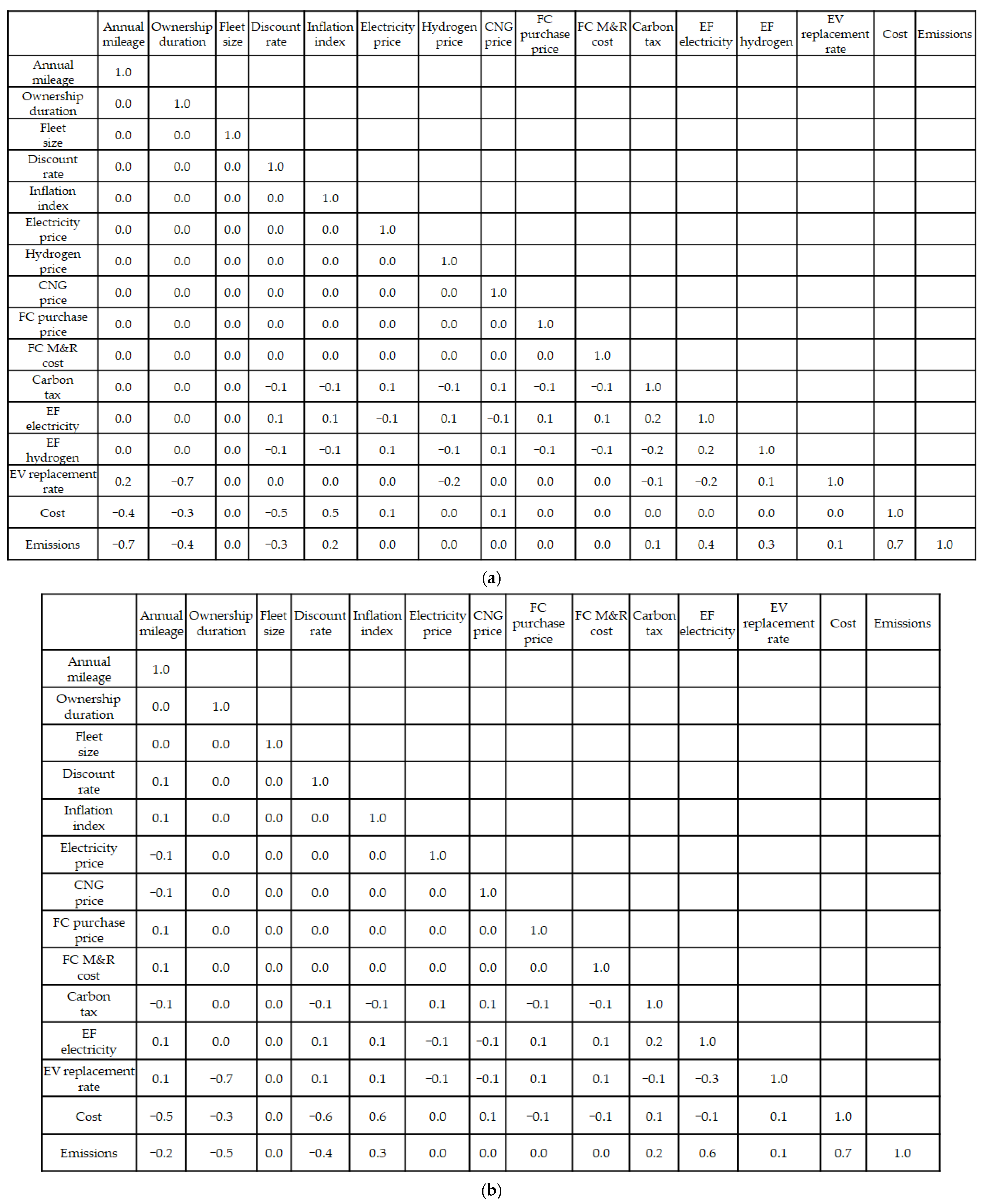
  • Cost and emissions per kilometer decrease when annual mileage increases. This is consistent with the increment of the EV replacement rate and the drop-off in the ownership period;
  • Despite higher discount rates penalizing EV vans, cost and emissions per kilometer decrease. On this matter, the values considered for the discount rate are not high enough to significantly reduce the EV replacement rate. In addition, when the inflation index increases, costs and emissions grow;
  • Electricity EF has a significant effect on emissions and, to a lesser extent, on the EV replacement rate;
  • Higher emissions are associated with higher costs per kilometer.
The evaluation of robustness has been carried out through a worst-case scenario analysis for the cases accounting for scope 3 emissions that have shown higher sensitivity to the variation in certain model parameters. In the H2P case (Table 12), the FCEREV van is optimal for higher annual mileage (above 30.000 km) and any van ownership period if the acquisition cost is equivalent to a BEV van. In this sense, the FCEV vans are penalized by the increase in the discount and inflation rate due to their higher purchase price. Moreover, in the H2G case (Table 13), the BEV van type is optimal for higher annual mileage (above 30.000 km) and any ownership period, and if the acquisition cost is cheaper than an FCEREV van (10%), it is also convenient in lower annual mileage (20.000 km).
Nevertheless, the FCEREV van is not the optimal powertrain type for low annual mileage (20.000 km) when the price of electricity decreases (10%), and the purchase and maintenance cost of fuel-cell powered vans increases (10%) or the hydrogen is produced on-site using electricity from the grid. Additionally, an increase in discount and inflation rates in shorter ownership periods (5 years) makes it no longer efficient to use electric vans.

4.4. Research Findings Summary

The results obtained in the simulations conducted over the Spanish market scenarios reveal interesting information to support the fleet managers’ action plan, providing insights into the following concerns:
  • The results obtained for the optimal solution (BAL) in the scenarios analyzed show that the most significant model parameters are the electricity EF, the yearly mileage, and the van’s ownership period, followed by the purchase price of fuel-cell-powered vans and the discount rate and inflation, whereas the fuel-cell-powered van maintenance cost and the electricity price show a lower effect. Concerning related hydrogen parameters, only H2P scenarios are affected. Hydrogen price is highly influenced in scenarios with higher yearly mileage, over 30.000 km. Nevertheless, the EF of blended hydrogen has a low effect;
  • The FCEREV vans achieve the right balance between emissions and the economy of use in a wide range of H2P and H2G scenarios. This type of van is suitable for moderate annual distances (up to 30.000 km) when scope 3 emissions are accounted for. Nevertheless, if scope 3 emissions are out of scope, then the optimal distance is reduced to 20.000 km. Meanwhile, the BEV vans are optimal for the H2G scenario for larger annual distances when scope 3 emissions are reported (over 40.000 km). Additionally, it should be noted that FCEV represents an optimal option in the H2P scenario with high annual mileage (over 40.000 km). However, if scope 3 emissions are not accounted for, BEVs are optimal for moderate distances (over 30.000 km). Thus, regardless of the higher purchase costs, EV vans are the best option with high utilization levels. These results are consistent with conclusions drawn in prior research works [14,23,62], but the breakeven distance is higher when scope 3 emissions are considered;
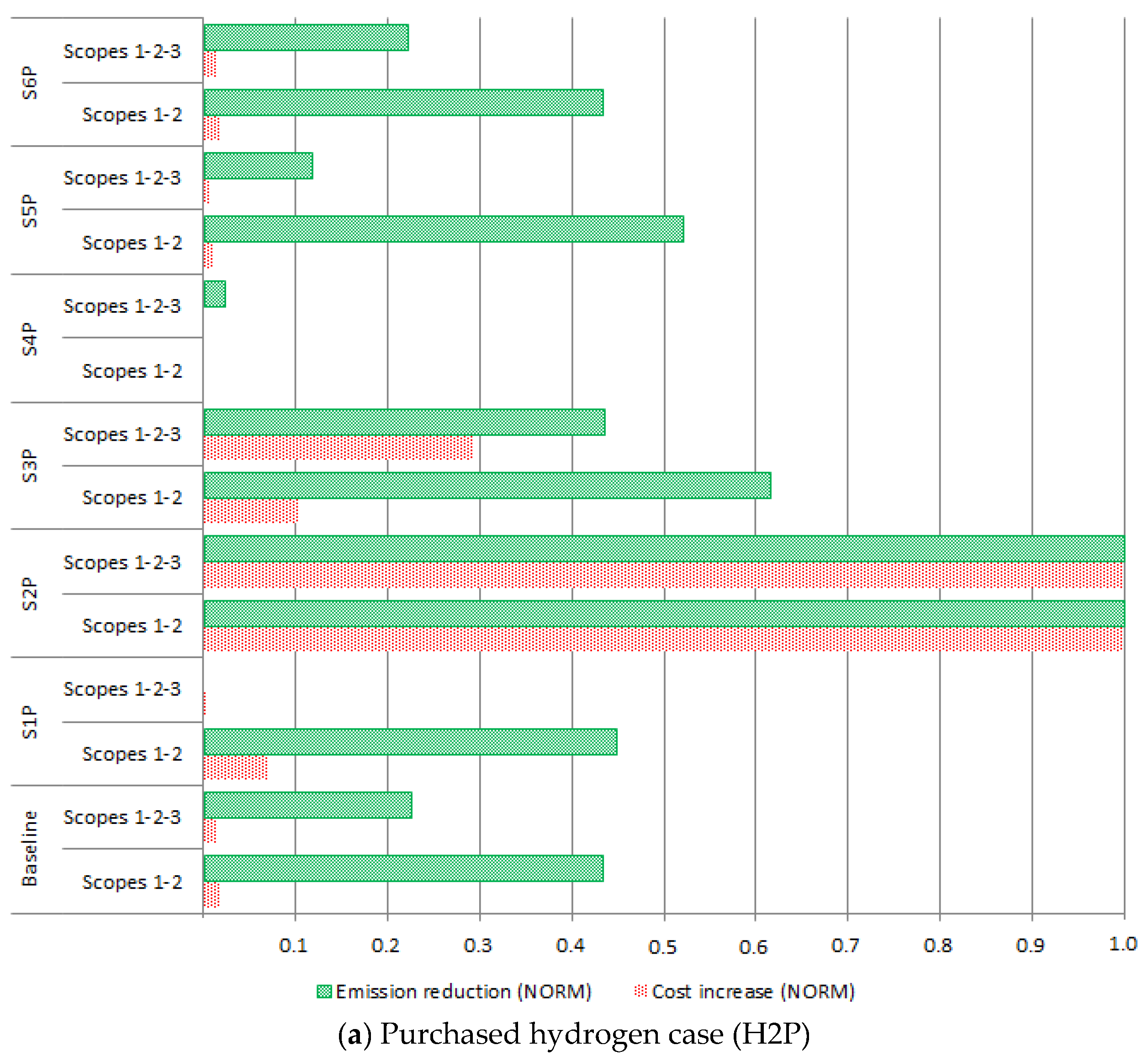
  • The average fleet emissions per kilometer are determined by yearly mileage, the van’s ownership period, the electricity production mix, and the hydrogen pathway. The emissions are higher in the H2G scenarios except for the scenarios with the lowest annual mileage (under 20.000 km). On average, the difference is 20.7% if the emissions scopes reported are 1 and 2 and 16% when the emissions in scope 3 are accounted for. Therefore, from the emissions inventorying point of view, the purchased hydrogen scenario (H2P) is the most favorable, and it is not efficient to use grid electricity to produce hydrogen by on-site electrolysis. As previous investigations’ outcomes show [14,23,58], the emissions from energy pathway production and distribution have important environmental implications, but they are more significant if scope 3 emissions are reported;
  • The consideration of scope 3 in the emissions report increases the level of accounted emissions by an average of over 71%. The emissions reported in scope 3 have approximately the same weight as the sum of the emissions accounted for in scopes 1 and 2, except for the S4 scenarios with the longest ownership period. Additionally, when scope 3 emissions are taken into account, the EV replacement rate is lower, and the fleet mix is affected. This aspect is especially noteworthy in H2G scenarios because of changes in the preferred van options from BEV to FC-EREV, except for the longest annual mileage (S2-G). These results point out the importance of the emissions generated during EV van manufacturing;
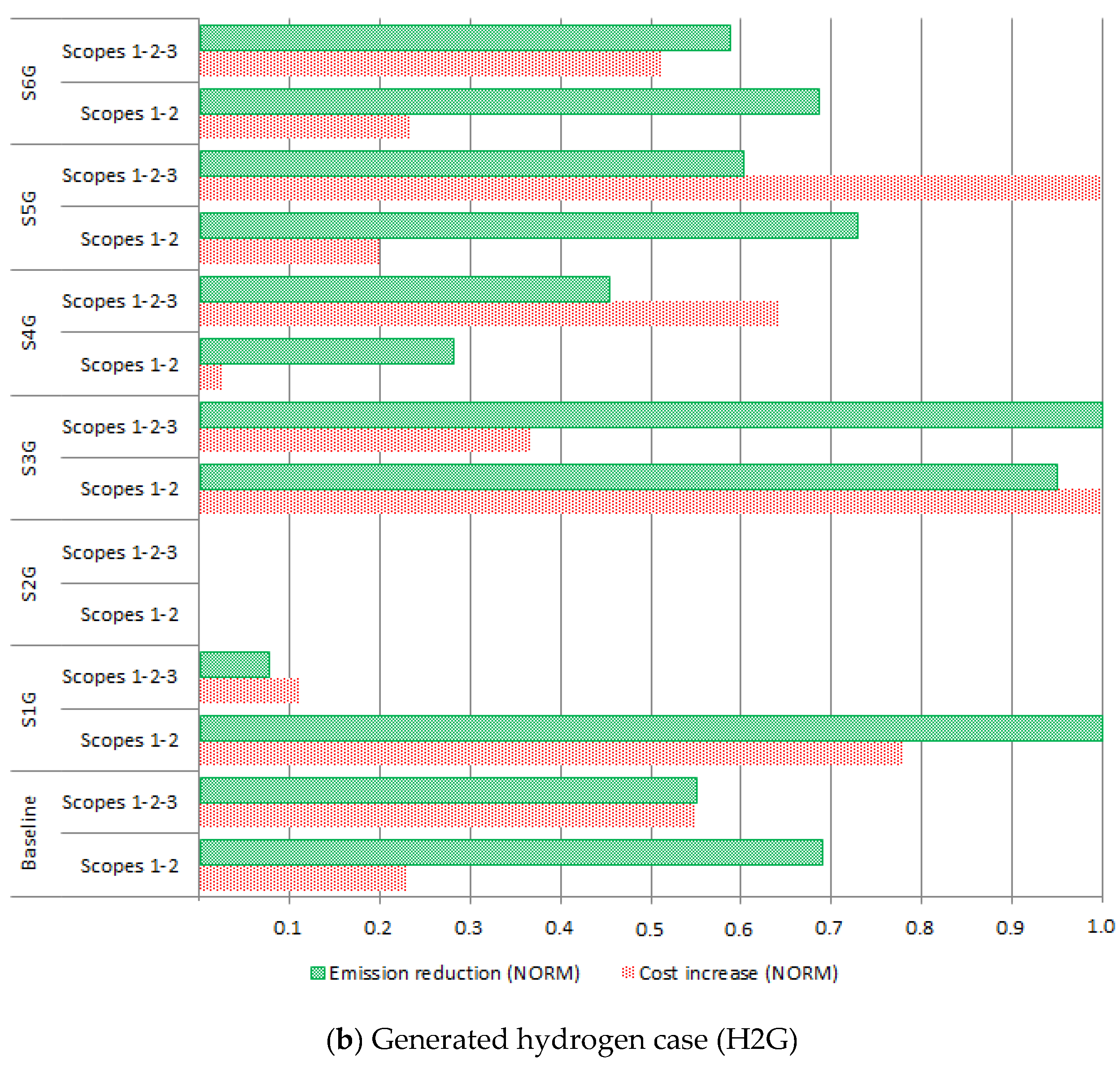
  • The average cost per kilometer is similar in the H2G and H2P scenarios, considering an average price for hydrogen and electricity of EUR 4.2/kg and EUR 168/MWh, but it is obtained with different van powertrains, BEV in the H2G scenarios and FCEREV in the H2P scenarios. With moderate annual mileage (below 30.000 km), long ownership periods (over 8 years), and a large number of vehicles in the fleet (over 200 vehicles), the FCEREV van is the best option with reductions in costs and emission levels to 2.7% and 18.5%, respectively, compared to BEV. Nevertheless, higher annual mileage (over 40.000 km) gives an advantage to the BEV vans with a cost reduction of 21.4% but with an emission increment of 41.4%. Furthermore, longer ownership periods (10 years) allow for reaching lower operating costs per kilometer. Additionally, the small fleet vans with fuel cell vans are more economically affected by the hydrogen supply infrastructure cost. Additionally, the smaller fleets with fuel cell vans are economically affected by the hydrogen supply infrastructure cost;
  • There is an emission–cost correlation, and there is a cost increase for reducing fleet emissions. This tendency is also observed in other previous studies [23,35,59]. However, the life cycle emissions structure is different for EV and CNG vans; while operation emissions are high for CNG vans compared to production emissions values, in EVs, it is quite the opposite [50,54]. This trend is observed in the distribution of emissions in scopes 2 and 3.

5. Conclusions

At present, a sustainable logistics approach has become essential for any company aspiring to achieve cost savings and cultivate a favorable image. The first step for implementing a sustainable logistic strategy is to calculate the corporate emissions to identify the emissions hotspots and implement action plans accordingly. On this subject, transportation companies have set the target of electrifying their last-mile delivery vehicles. The adoption of electric vans for urban delivery activities requires a holistic approach to select the most favorable replacement strategy. To reach this goal, the authors have innovated by combining the fleet parallel replacement problem with the corporate greenhouse gas emissions reporting according to the GHG Protocol standards in a MOLP model. This investigation brings the chance for fleet managers to evaluate the carbon footprint impact of transport activity and analyze the cost-effective behavior of the van fleet. In this sense, the fleet operator could select the replacement calendar with the most suitable van type and refueling infrastructure characteristics, fulfilling the economic and environmental corporation objectives.
In addition, the optimization model has been tested in a multi-scenario approach applied to the Spanish market for evaluating multiple electrified powertrain vans. The findings derived from the present research study lead to the following conclusions that may be useful for policy recommendation, mitigating environmental impacts, and enhancing the cost-effectiveness of LCVs in last-mile delivery:
  • The uptake of electric vans for last-mile delivery activity is strongly dependent on the energy emission factor. The reduction in electricity mix EF (under 0.1 kgCO2e/kWh) enables several types of electric powertrains to participate in the fleet mix. On the other hand, the EF of blended hydrogen has a low effect. In this sense, the use of this type of hydrogen for transportation can accelerate the penetration of fuel-cell commercial vehicles in the market;
  • Energy price has a strong influence on the competitiveness of electric vans in scenarios with higher yearly mileages (over 30.000 km). In the case of electricity, the price should be under EUR 0.17/kWh. Meanwhile, the hydrogen cost should be under EUR 4.6/kg;
  • The FCEREV vans achieve the right balance between emissions and the economy of use in a wide range of scenarios. This type of van is suitable for moderate annual distances (up to 30.000 km) when scope 3 emissions are accounted for. Nevertheless, if scope 3 emissions are out of scope, then the optimal distance is reduced to 20.000 km. Additionally, it should be noted that FCEV is an optimal option in the H2P scenario with high annual mileage (over 40.000 km);
  • The BEV vans are optimal in H2G scenarios for larger annual distances (over 40.000 km). However, if scope 3 emissions are not accounted for, BEVs are optimal for moderate distances (over 30.000 km);
  • The emissions are higher in the H2G scenarios except for the scenarios with the lowest annual mileage (under 20.000 km). Therefore, from the emissions inventorying point of view, the purchased hydrogen scenario (H2P) is the most favorable, and it is not efficient to use grid electricity to produce hydrogen by on-site electrolysis with the actual electricity mix EF (0.25 kgCO2e/kWh);
  • In the accounting of scope 3 emissions in the corporate report, the fleet mix is affected, and the EV replacement rate is lower. This aspect is especially noteworthy for BEV vans in scenarios with moderate annual mileage (under 40.000 km);
  • The consideration of scope 3 emissions raises the importance of the emissions generated during EV van manufacturing and energy production and distribution pathway. In this sense, the organization has a better understanding of the full GHG impact of their operations.
This new approach to solving vehicle replacement issues in urban delivery fleets can be applied to a wide range of van fleet typologies for transport agencies located in different European countries. By using this optimization approach, fleet managers can make simulations to identify patterns and trends to build up policies for planning future fleet mixes and refueling infrastructure needs.
Limitations of this study lie basically in the values of the model parameters under consideration. Accordingly, due to the technological maturity of the vehicles and energy supply means used in this study, it is necessary to revise the model data to establish their effects in terms of environmental and economic performances over time. Moreover, the environmental parameters of this model should be updated depending on the location of this study. From this point of view, the developed model is sensitive to adjustments in the parameter values, the vehicle types and infrastructure assets, and fleet management requirements, such as budget, initial fleet conditions (the age and the number of vehicles and energy supply assets), daily distance demand and van’s ownership period.
Future research works should have the potential to broaden the scope in exploring the environmental performance and competitive costs of alternative electric vehicle options, including more categories in scope 3 emissions and long-term forecasting of energy and vehicle prices and energy EF. In addition, it could be of interest to make cross-national comparative studies for defining future EU regulations. Furthermore, this optimization model might be explored to identify technological advancements in powertrain systems or refueling infrastructures that significantly impact the environmental and economic performance of vehicles.
Therefore, these findings have practical implications for building realizable fleet management action plans and selecting adequate corporate emissions reporting methodology for logistics companies. Additionally, these findings open up consequences on the corporate emissions inventory of the hydrogen supply pathway. These concerns are of interest not only to fleet managers but also to policymakers. Finally, an assessment could also be made of the fleet change in an entire country by considering the actual vehicle fleet and analyzing how the fleet of the future would be more or less dependent on fossil fuel, hydrogen, or electricity.

Author Contributions

Conceptualization, O.C. and R.Á.; Methodology, O.C. and R.Á.; Software, O.C.; Writing—original draft, O.C.; Writing—review & editing, R.Á.; Supervision, R.Á. All authors have read and agreed to the published version of the manuscript.

Funding

This research received no external funding.

Institutional Review Board Statement

Not applicable.

Informed Consent Statement

Not applicable.

Data Availability Statement

Data are contained within the article.

Conflicts of Interest

The authors declare no conflict of interest.

Abbreviations

LCompressed natural gasLCALife cycle assessment
EFEmission factorLCCLife cycle cost
EVElectric VehicleLCVLight commercial vehicle
GLFGrid loss factorMILPMixed Integer Linear Programming
BEVBattery electric vehicleMOLPMulti-Objective Linear Programming
FCEVFuel cell electric vehicleM&RMaintaining and repairing
FCEREVFuel cell extended range electric vehiclePHEVPlug-in hybrid electric vehicle
GHGGreenhouse gasPVPassenger vehicle
HEVHybrid electric vehicleSMRSteam Methane Reforming
HRSHydrogen refueling stationTDCOTotal Discounted Cost of Ownership
ICEInternal combustion engine

References

  1. European Environment Agency. EEA Transport and Environment Report 2022. Digitalisation in the Mobility System: Challenges and Opportunities; European Environment Agency: Copenhagen, Denmark, 2022. [Google Scholar]
  2. UNFCCC. National Inventory Submissions. Available online: https://unfccc.int/process-and-meetings/transparency-and-reporting/reporting-and-review-under-the-convention/national-inventory-submissions-2022 (accessed on 29 November 2023).
  3. European Commission. The EU Emissions Trading System (EU ETS). Available online: https://climate.ec.europa.eu/eu-action/eu-emissions-trading-system-eu-ets_en (accessed on 10 January 2023).
  4. Schroten, A.; Julius, K.; Scholten, P. Research for TRAN Committee—Pricing Instruments on Transport Emissions; European Parliament, Policy Department for Structural and Cohesion Policies: Brussels, Belgium, 2022. [Google Scholar]
  5. European Commission. White Paper: Roadmap to a Single European Transport Area—Towards a Competitive and Resource Efficient Transport System; European Commission: Brussels, Belgium, 2011. [Google Scholar]
  6. Aditjandra, P.T.; Galatioto, F.; Bell, M.C.; Zunder, T.H. Evaluating the Impacts of Urban Freight Traffic: Application of Micro-Simulation at a Large Establishment. Eur. J. Transp. Infrastruct. Res. 2016, 16, 4–22. [Google Scholar] [CrossRef]
  7. Asociación de Fabricantes y Distribuidores (AECOC). Los Impactos Nocivos del Transporte Urbano en España. Available online: https://www.aecoc.es/noticias/los-impactos-nocivos-del-transporte-urbano-en-espana-suponen-un-coste-economico-del-2-sobre-el-pib/ (accessed on 21 June 2022).
  8. Lean & Green.Lean and Green Program. Available online: https://www.lean-green.eu/program_co2_action_plan/ (accessed on 21 December 2021).
  9. The Last-Mile Delivery Challenge; Capgemini Research Institute: Paris, France, 2019.
  10. Seroka-Stolka, O. The Development of Green Logistics for Implementation Sustainable Development Strategy in Companies. Procedia—Soc. Behav. Sci. 2014, 151, 302–309. [Google Scholar] [CrossRef]
  11. Evangelista, P.; Colicchia, C.; Creazza, A. Is Environmental Sustainability a Strategic Priority for Logistics Service Providers? J. Environ. Manag. 2017, 198, 353–362. [Google Scholar] [CrossRef] [PubMed]
  12. Di Foggia, G. Drivers and Challenges of Electric Vehicles Integration in Corporate Fleet: An Empirical Survey. Res. Transp. Bus. Manag. 2021, 41, 100627. [Google Scholar] [CrossRef]
  13. Albitar, K.; Al-Shaer, H.; Liu, Y.S. Corporate Commitment to Climate Change: The Effect of Eco-Innovation and Climate Governance. Res. Policy 2023, 52, 104697. [Google Scholar] [CrossRef]
  14. Alp, O.; Tan, T.; Udenio, M. Transitioning to Sustainable Freight Transportation by Integrating Fleet Replacement and Charging Infrastructure Decisions. Omega 2022, 109, 102595. [Google Scholar] [CrossRef]
  15. Tanco, M.; Cat, L.; Garat, S. A Break-Even Analysis for Battery Electric Trucks in Latin America. J. Clean. Prod. 2019, 228, 1354–1367. [Google Scholar] [CrossRef]
  16. Van Mierlo, J.; Messagie, M.; Rangaraju, S. Comparative Environmental Assessment of Alternative Fueled Vehicles Using a Life Cycle Assessment. Transp. Res. Procedia 2017, 25, 3439–3449. [Google Scholar] [CrossRef]
  17. Bicer, Y.; Dincer, I. Life Cycle Environmental Impact Assessments and Comparisons of Alternative Fuels for Clean Vehicles. Resour. Conserv. Recycl. 2018, 132, 141–157. [Google Scholar] [CrossRef]
  18. Del Pero, F.; Delogu, M.; Pierini, M. Life Cycle Assessment in the Automotive Sector: A Comparative Case Study of Internal Combustion Engine (ICE) and Electric Car. Procedia Struct. Integr. 2018, 12, 521–537. [Google Scholar] [CrossRef]
  19. Marmiroli, B.; Venditti, M.; Dotelli, G.; Spessa, E. The Transport of Goods in the Urban Environment: A Comparative Life Cycle Assessment of Electric, Compressed Natural Gas and Diesel Light-Duty Vehicles. Appl. Energy 2020, 260, 114236. [Google Scholar] [CrossRef]
  20. Onat, N.C.; Abdella, G.M.; Kucukvar, M.; Kutty, A.A.; Al-Nuaimi, M.; Kumbaroğlu, G.; Bulu, M. How Eco-Efficient Are Electric Vehicles across Europe? A Regionalized Life Cycle Assessment-Based Eco-Efficiency Analysis. Sustain. Dev. 2021, 29, 941–956. [Google Scholar] [CrossRef]
  21. Scorrano, M.; Danielis, R.; Giansoldati, M. Electric Light Commercial Vehicles for a Cleaner Urban Goods Distribution. Are They Cost Competitive? Res. Transp. Econ. 2021, 85, 101022. [Google Scholar] [CrossRef]
  22. Feng, W.; Figliozzi, M. An Economic and Technological Analysis of the Key Factors Affecting the Competitiveness of Electric Commercial Vehicles: A Case Study from the USA Market. Transp. Res. Part C Emerg. Technol. 2013, 26, 135–145. [Google Scholar] [CrossRef]
  23. Zhao, Y.; Ercan, T.; Tatari, O. Life Cycle Based Multi-Criteria Optimization for Optimal Allocation of Commercial Delivery Truck Fleet in the United States. Sustain. Prod. Consum. 2016, 8, 18–31. [Google Scholar] [CrossRef]
  24. Al-dal’ain, R.; Celebi, D. Planning a Mixed Fleet of Electric and Conventional Vehicles for Urban Freight with Routing and Replacement Considerations. Sustain. Cities Soc. 2021, 73, 103105. [Google Scholar] [CrossRef]
  25. Karaman, A.S.; Kilic, M.; Uyar, A. Green Logistics Performance and Sustainability Reporting Practices of the Logistics Sector: The Moderating Effect of Corporate Governance. J. Clean. Prod. 2020, 258, 120718. [Google Scholar] [CrossRef]
  26. Ortiz-Martínez, E.; Marín-Hernández, S.; Santos-Jaén, J.-M. Sustainability, Corporate Social Responsibility, Non-Financial Reporting and Company Performance: Relationships and Mediating Effects in Spanish Small and Medium Sized Enterprises. Sustain. Prod. Consum. 2023, 35, 349–364. [Google Scholar] [CrossRef]
  27. Schiffer, M.; Klein, P.S.; Laporte, G.; Walther, G. Integrated Planning for Electric Commercial Vehicle Fleets: A Case Study for Retail Mid-Haul Logistics Networks. Eur. J. Oper. Res. 2021, 291, 944–960. [Google Scholar] [CrossRef]
  28. GreenHouse Gas Protocol. GHG Protocol—Calculation Tools. Available online: https://ghgprotocol.org/calculation-tools (accessed on 23 June 2022).
  29. Redmer, A. Strategic Vehicle Fleet Management–A Joint Solution of Make-or-Buy, Composition and Replacement Problems. J. Qual. Maint. Eng. 2020, 28, 327–349. [Google Scholar] [CrossRef]
  30. Lee, D.Y.; Thomas, V.M.; Brown, M.A. Electric Urban Delivery Trucks: Energy Use, Greenhouse Gas Emissions, and Cost-Effectiveness. Environ. Sci. Technol. 2013, 47, 8022–8030. [Google Scholar] [CrossRef] [PubMed]
  31. Giordano, A.; Fischbeck, P.; Matthews, H.S. Environmental and Economic Comparison of Diesel and Battery Electric Delivery Vans to Inform City Logistics Fleet Replacement Strategies. Transp. Res. Part D Transp. Environ. 2018, 64, 216–229. [Google Scholar] [CrossRef]
  32. Lal, A.; Renaldy, T.; Breuning, L.; Hamacher, T.; You, F. Electrifying Light Commercial Vehicles for Last-Mile Deliveries: Environmental and Economic Perspectives. J. Clean. Prod. 2023, 416, 137933. [Google Scholar] [CrossRef]
  33. Figliozzi, M.A.; Boudart, J.A.; Feng, W. Economic and Environmental Optimization of Vehicle Fleets. Transp. Res. Rec. 2011, 2252, 1–6. [Google Scholar] [CrossRef]
  34. Feng, W.; Figliozzi, M. Vehicle Technologies and Bus Fleet Replacement Optimization: Problem Properties and Sensitivity Analysis Utilizing Real-World Data. Public Transp. 2014, 6, 137–157. [Google Scholar] [CrossRef]
  35. Lemme, R.F.F.; Arruda, E.F.; Bahiense, L. Optimization Model to Assess Electric Vehicles as an Alternative for Fleet Composition in Station-Based Car Sharing Systems. Transp. Res. Part D Transp. Environ. 2019, 67, 173–196. [Google Scholar] [CrossRef]
  36. Islam, A.; Lownes, N. When to Go Electric? A Parallel Bus Fleet Replacement Study. Transp. Res. Part D Transp. Environ. 2019, 72, 299–311. [Google Scholar] [CrossRef]
  37. ISO 14040:2006; ISO Environmental Management—Life Cycle Assessment—Principles and Framework. ISO: Geneva, Switzerland, 2004; Volume 3, p. 32.
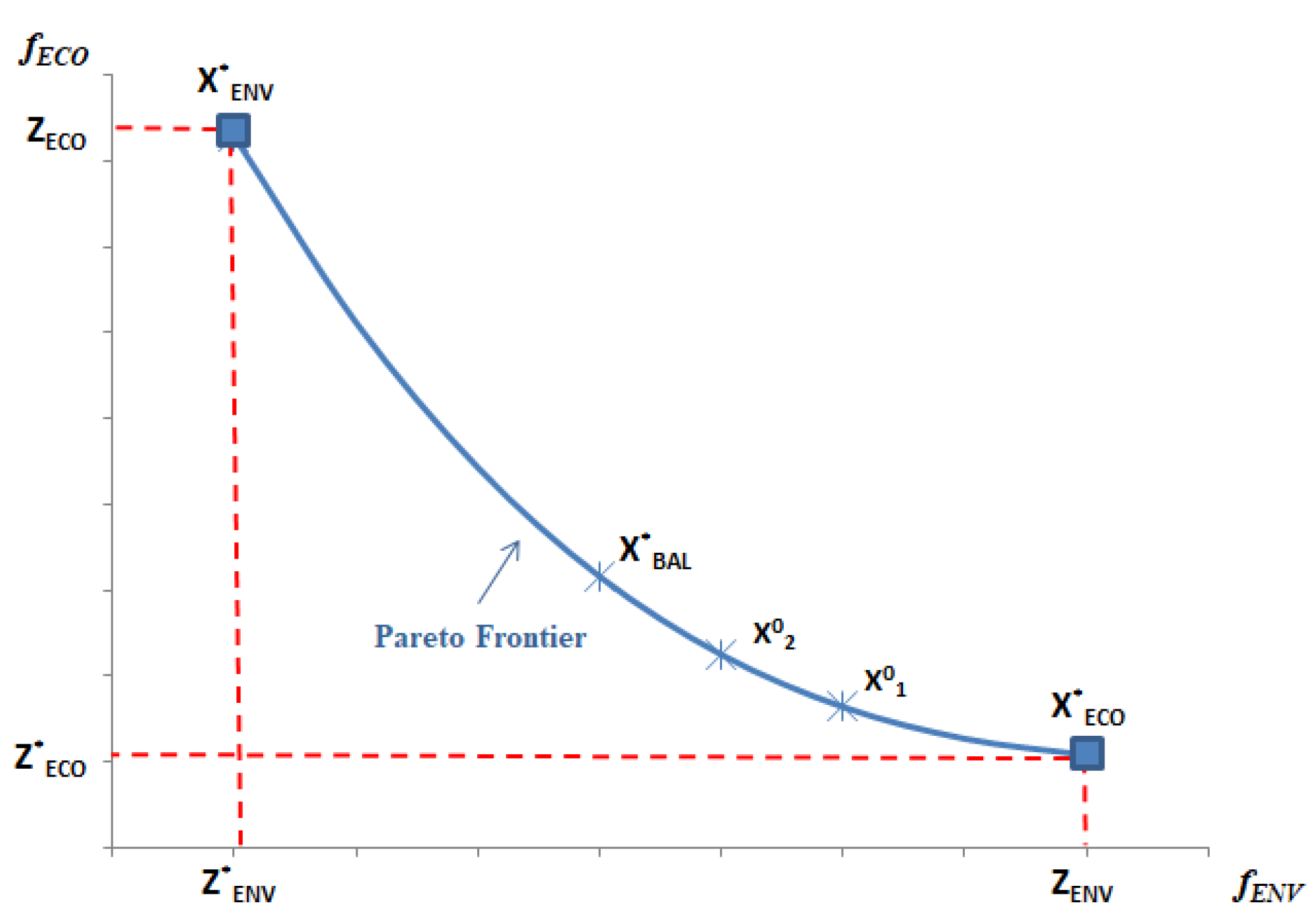
  38. Marler, R.T.; Arora, J.S. Survey of Multi-Objective Optimization Methods for Engineering. Struct. Multidiscip. Optim. 2004, 26, 369–395. [Google Scholar] [CrossRef]
  39. Shahriari, M.; Ehsanifar, M.; Rokhsati, A. Selecting the Most Preferable Weights in Multi Objective Programming. Am. J. Sci. Res. 2011, 28, 87–92. [Google Scholar]
  40. Schmied, M.; Knörr, W.; Friedl, C.; Hepburn, L. Calculating GHG Emissions for Freight Forwarding and Logistics Services; European Association for Forwarding, Transport, Logistics and Customs Services (CLECAT): Brussels, Belgium, 2012. [Google Scholar]
  41. Wulf, C.; Kaltschmitt, M. Hydrogen Supply Chains for Mobility-Environmental and Economic Assessment. Sustainability 2018, 10, 1699. [Google Scholar] [CrossRef]
  42. Bareiß, K.; de la Rua, C.; Möckl, M.; Hamacher, T. Life Cycle Assessment of Hydrogen from Proton Exchange Membrane Water Electrolysis in Future Energy Systems. Appl. Energy 2019, 237, 862–872. [Google Scholar] [CrossRef]
  43. E4tech H2 Emission Potential Literature Review; Department for Business Energy and Industrial Strategy (BEIS): London, UK. 2019. Available online: https://assets.publishing.service.gov.uk/media/5cc6f1e640f0b676825093fb/H2_Emission_Potential_Report_BEIS_E4tech.pdf (accessed on 10 January 2023).
  44. IPCC. Climate Change 2007: Synthesis Report. Contribution of Working Groups I, II and III to the Fourth Assessment Report of the Intergovernmental Panel on Climate Change; IPCC: Geneva, Switzerland, 2007. [Google Scholar]
  45. Ministerio de Industria y Energía. Factores de Emisión de CO2 y Coeficientes de Paso a Energía Primaria de Diferentes Fuentes de Energía Final En El Sector de Edificios En España; Ministerio de Industria, Energía y Turismo: Madrid, España, 2014. [Google Scholar]
  46. IEA Emission Factors 2020—Data Base Documentation. 2020. Available online: https://iea.blob.core.windows.net/assets/24422203-de22-4fe6-8d54-f51911addb8b/CO2KWH_Methodology.pdf (accessed on 10 January 2023).
  47. DOE. Hydrogen Delivery. Fuel Cell Technologies; Office Multi-Year Research, Development and Demonstration Plan. 2015. Available online: https://www.energy.gov/sites/default/files/2015/08/f25/fcto_myrdd_delivery.pdf (accessed on 10 January 2023).
  48. Ligen, Y.; Vrubel, H.; Girault, H.H. Mobility from Renewable Electricity: Infrastructure Comparison for Battery and Hydrogen Fuel Cell Vehicles. World Electr. Veh. J. 2018, 9, 3. [Google Scholar] [CrossRef]
  49. Ramsden, T.; Ruth, M.; Diakov, V. Hydrogen Pathways: Cost, Well-to-Wheels Energy Use, and Emissions for the Current Technology Status of 10 Hydrogen Production, Delivery, and Distribution Scenarios; National Renewable Energy Laboratory (NREL): Denver, CO, USA, 2013. [Google Scholar]
  50. Buberger, J.; Kersten, A.; Kuder, M.; Eckerle, R.; Weyh, T.; Thiringer, T. Total CO2-Equivalent Life-Cycle Emissions from Commercially Available Passenger Cars. Renew. Sustain. Energy Rev. 2022, 159, 112158. [Google Scholar] [CrossRef]
  51. Castillo Campo, O.; Álvarez Fernández, R. Economic Optimization Analysis of Different Electric Powertrain Technologies for Vans Applied to Last Mile Delivery Fleets. J. Clean. Prod. 2023, 385, 135677. [Google Scholar] [CrossRef]
  52. Secretaría de Estado de Medio Ambiente. Emisiones de Gases de Efecto Invernadero, 1999–2020; Ministerio para la Transición Ecológica y el Reto Demográfico (MITECO): Madrid, España, 2022. [Google Scholar]
  53. Red Electrica de España (REE). La Eólica se Convierte en la Principal Fuente de Generación de Energía Eléctrica en España en 2021. Available online: https://www.ree.es/es/sala-de-prensa (accessed on 18 July 2022).
  54. Simons, S.; Azimov, U. Comparative Life Cycle Assessment of Propulsion Systems for Heavy-Duty Transport Applications. Energies 2021, 14, 3079. [Google Scholar] [CrossRef]
  55. Bieker, G. A Global Comparison of the Life-Cycle Greenhouse Gas Emissions of Combustin Engine and Electric Passenger Cars; The International Council on Clean Transportation (ICCT): Berlin, Germany, 2021. [Google Scholar]
  56. Yeow, L.W.; Yan, Y.; Cheah, L. Life Cycle Greenhouse Gas Emissions of Alternative Fuels and Powertrains for Medium-Duty Trucks: A Singapore Case Study. Transp. Res. Part D Transp. Environ. 2022, 105, 103258. [Google Scholar] [CrossRef]
  57. Qiao, Q.; Zhao, F.; Liu, Z.; Jiang, S.; Hao, H. Comparative Study on Life Cycle CO2 Emissions from the Production of Electric and Conventional Vehicles in China. Energy Procedia 2017, 105, 3584–3595. [Google Scholar] [CrossRef]
  58. Bauer, C.; Hofer, J.; Althaus, H.J.; Del Duce, A.; Simons, A. The Environmental Performance of Current and Future Passenger Vehicles: Life Cycle Assessment Based on a Novel Scenario Analysis Framework. Appl. Energy 2015, 157, 871–883. [Google Scholar] [CrossRef]
  59. Desantes, J.M.; Novella, R.; Pla, B.; Lopez-Juarez, M. Impact of Fuel Cell Range Extender Powertrain Design on Greenhouse Gases and NOX Emissions in Automotive Applications. Appl. Energy 2021, 302, 117526. [Google Scholar] [CrossRef]
  60. Usai, L.; Hung, C.R.; Vásquez, F.; Windsheimer, M.; Burheim, O.S.; Strømman, A.H. Life Cycle Assessment of Fuel Cell Systems for Light Duty Vehicles, Current State-of-the-Art and Future Impacts. J. Clean. Prod. 2021, 280, 125086. [Google Scholar] [CrossRef]
  61. The World Bank. State and Trends of Carbon Pricing 2021; World Bank: Washington, DC, USA, 2021. [Google Scholar] [CrossRef]
  62. Li, M.; Zhang, X.; Li, G. A Comparative Assessment of Battery and Fuel Cell Electric Vehicles Using a Well-to-Wheel Analysis. Energy 2016, 94, 693–704. [Google Scholar] [CrossRef]
Figure 1. Research methodology scheme.
Sustainability 15 16909 g001
Figure 2. Example of Pareto frontier for the proposed bi-objective problem.
Sustainability 15 16909 g002
Figure 3. The replacement rate and fleet share for the BAL solution in all the scenarios analyzed.
Sustainability 15 16909 g003
Figure 4. The replacement rate and fleet share for the ECON solution in all the scenarios analyzed.
Sustainability 15 16909 g004
Figure 5. The replacement rate and fleet share for the ENV solution in all the scenarios analyzed.
Sustainability 15 16909 g005
Figure 6. Average cost and emissions per kilometer and the emissions per scope for the BAL solutions in all the scenarios analyzed.
Sustainability 15 16909 g006aSustainability 15 16909 g006b
Figure 7. Emission savings and cost increase for the BAL solutions compared to the ECON solutions in all the scenarios analyzed.
Sustainability 15 16909 g007aSustainability 15 16909 g007b
Figure 8. Correlation matrix for the BAL solution with scope 3 reporting. (a) Acquired hydrogen case (H2—P); (b) On-site electrolysis produced hydrogen case (H2—G).
Sustainability 15 16909 g008
Table 1. Optimal fleet replacement with emissions concerns in the literature.
Ref.MethodEconomic
Evaluation
GHG EvaluationScope of Vehicle Emissions AnalysisVehicle TypePowertrain
TDCOLCCCost
(CS)
Emissions (EM)OPLCAECR BEVFCEVICEAlternatives
[33]LP-SOX X X PVX XHEV
[22]LP-SOX X X LCVX X
[34]LP-SOX X X Bus XHEV
[23]LP-MO X X X LCVX XHEV
CNG
[35]LP-MOX X X PVX XPHEV
[36]LP-SOX X X BusX X
[24]LP-SOX X X LCVX X
Study
contribution
LP-MOX X XLCVXXXFCEREV
CNG
Note: (TDCO) Total Discounted Cost of Ownership; (LCC) Life Cycle Cost; (OP) Emissions during vehicle operation; (LCA) Emissions life cycle assessment; (ECR) Emissions Corporate GHG Report; (CS) GHG emissions are converted to a function cost using a carbon tax; (EM) The objective function uses only GHG emissions indicators.
Table 2. Indices used in the mathematical model.
IndexRangeDescriptionUnits
i0 to NkThe age of the vanYear
j0 to TThe current year in the planning horizonYear
kk = 1 (van CNG); k = 2 (van BEV);
k = 3 (van FCEREV); k = 4 (van FCEV)
The van’s powertrain typeDimensionless
m0 to NrThe age of the energy supply infrastructureYear
rr = 1 (charging point for BEV);
r = 2 (charging point for FCEREV);
r = 3 (HRS for FCEREV bought or produced);
r = 4 (HRS for FCEV bought or produced);
r = 5 (FCEV and FCEREV hydrogen dispenser)
The energy supply infrastructure typeDimensionless
Table 3. Parameters used in the mathematical model.
ParameterDescriptionUnits
NkVan type “k” ownership period in the fleet. It is possible to set up different ownership periods for each van type (CNG, BEV, FCEREV, and FCEV).Year
TPlanning horizon analyzed.Year
Nr“r” type energy supply infrastructure asset service life. Each r-type energy supply device has a different service life.Year
rifInflation index.Dimensionless
rdDiscount rate (nominal value).Dimensionless
APVjkThe acquisition price in the year “j” of a van type “k”. EUR/van
VDRikType “k” van “i” years old depreciation factor.Dimensionless
FCijkFixed term of operating costs in the year “j” for a type “k” van “i” years old.EUR/year
VECijkFueling costs during the year “j” for a type “k” van “i” years old.EUR/km
MCVijkCost of van’s maintenance in the year “j” for a type “k” van “i” years old. EUR/km
RCVijkCost of van’s repair in the year “j” for a type “k” van “i” years old. EUR/km
AMijkAnnual mileage demand in the year “j” for a type “k” van “i” years old. km/year
APIjr“r” type energy supply infrastructure asset acquisition price in the year “j”.EUR/infrastructure
ISRmr“r” type energy supply infrastructure asset scrapping return value with “m” years of operation.Dimensionless
MCImjr“r” type energy supply infrastructure asset maintenance costs in the year “j” with “m” years of operation.EUR/year
RCImjr“r” type energy supply infrastructure asset repairing costs in the year “j” with “m” years of operation.EUR/year
E Q 1 C N G Scope 1 GHG emissions based on the CNG consumption.kgCO2e
C E P j Emission tax in the year “j”.EUR/kgCO2e
E C N G Yearly van CNG consumption.kg
E Q 2 E V k Scope 2 GHG emissions associated with the purchased electricity. kgCO2e
E e k Yearly electricity consumption of each van of type “k”. There are only two plug-in vans: BEV (k = 2); and FCEREV (k = 3).kWh
E Q 3 V A N k Scope 3 GHG emissions produced by the electricity acquired (reported in scope 2) due to transmission and distribution losses.kgCO2e
E Q 3 H 2 k Scope 3 GHG emissions based on the hydrogen purchased.kgCO2e
E H 2 k Yearly hydrogen consumption of each van of type “k” n. There are only two vans powered by hydrogen: FCEREV (k = 3); and FCEV (k = 4).kg
NSIr“r” type energy supply asset capacity for fueling vans per day.van
PVbjBudget for van purchasing during the year “j”.EUR
PIbjThe budgetary limit in the year “j” for purchasing an energy supply infrastructure asset. EUR
Table 4. Decision variables used in this mathematical model.
VariableDescription
VOijkVan “k” type “i” years old in operation during the year “j”.
VSijkVan “k” type “i” years old sold during the year “j”.
VAjkVan “k” type acquired during the year “j”.
IOmjrEnergy supply infrastructure asset “r” type with “m” years in operation during the year “j”.
ISmjrEnergy supply infrastructure asset “r” type with “m” years sold during the year “j”.
IAjrEnergy supply infrastructure asset “r” type acquired during the year “j”.
Table 5. Scenarios analyzed.
Modeling VariablesUnitsScenario Nomenclature
BaselineS1 (P/G)S2 (P/G)S3 (P/G)S4 (P/G)S5 (P/G)S6 (P/G)
Hydrogen supply pathway H2 acquired (P) or H2 on-site electrolysis produced (G)
Corporate emissions reporting option Scopes 1 and 2 (S12) or scopes 1, 2, and 3 (S123)
Annual mileagekm30.00020.00040.00030.00030.00030.00030.000
Van’s ownership
period
years88851088
Fleet sizeunits20020020020020080320
Table 6. Economic data.
CNGBEVFCEREVFCEVComments
Discount rate%2.5---(1)
Inflation index%1.3---(1)
Van acquisition costEUR/van37.38551.52051.86571.450(2)
Maintenance cost (4)EUR/km0.180.090.110.11
Electricity cost (5)EUR/MWh 168--(3)
Hydrogen cost (5)EUR/kg--4.24.2
CNG cost (5)EUR/kg2.7---
Table notes: (1) Common value for all van types; (2) The price of electric vans is projected to rise in a manner that will maintain the initial price gap observed at the beginning of the planning horizon; (3) Common value for all vans with an electric powertrain; (4) Average maintenance cost calculated over time of the planning horizon; (5) Average energy price calculated over time of the planning horizon. Reference: [51].
Table 7. Energy EF factors used for scopes 1, 2, and 3.
EFCommentsReferences
CNG ( E F C N G )kgCO2e/kg2.8 [28,52]
Electricity ( E F e ) kgCO2e/kWh0.25(1)[53]
Diesel ( E F d i e s e l ) kgCO2e/L2.39(2)[28,52]
Hydrogen produced by SMR ( E F H 2 _ S M R ) kgCO2e/kg11.8 [41,54]
Table notes: (1) Spanish electricity production mix EF with a renewable energy contribution of 46.6%; (2) The EF considered is for a B10 diesel-type fuel.
Table 8. Van characteristics.
CNGBEVFCEREVFCEVComments
Van model Fiat Ducato L1H1Peugeot e-Expert --(1)
Powertrain powerkW101.4100100100
Fuel-cell stack powerkW--30100
Storage capacitykg36-1.53
Battery capacitykWh-75282
Vehicle body weightkg15661576.41576.41576.4
Powertrain weightkg13528.628.628.6
FC stack and peripheral components’ weightkg--2560
Fuel tank weightkg194-2653
Battery pack weightkg-48318012
Table notes: (1) The fuel cell models utilized in this study are derived from Peugeot e-Expert but with adaptations made to incorporate powertrain components sourced from the Toyota Mirai. References: [51].
Table 9. Manufacturing EF factors considered for vehicle components in scope 3.
EFCommentsReferences
Vehicle chassiskgCO2e/kg4.5 [50,55,56,57]
ICE motorkgCO2e/kg8(1)[57]
Electric motorkgCO2e/kW17 [55,58]
Traction batterykgCO2e/kWh158 [50,55,56,59]
Fuel cell systemkgCO2e/kW57 [56,59,60]
High-pressure hydrogen tankkgCO2e/kgH2640 [56,59,60]
CNG tankkgCO2e/kg8(1)[58]
Table notes: (1) Own assumption based on the literature data.
Table 10. Sensitivity analysis results in H2P scenarios for the BAL solutions.
Parameters Baseline Scenario
Scopes 1–2
Baseline Scenario Scopes 1–2–3
UnitsValue in the Baseline ScenarioValue for Sensitivity AnalysisE (1)SVO (2)ESVO
Annual mileagekm30.00020.000−0.26FCEREV−0.26FCEREV
km30.00040.000−0.51FCEREV−0.86MIX (6)
Van’s ownership
period
year850.49FCEREV−0.39FCEREV
year8100.33FCEREV−0.24FCEREV
Discount rate%2.506−0.37FCEREV−0.36FCEREV
Inflation indexwf (3)12.500.31FCEREV0.31FCEREV
Electricity price (4)EUR/kWh0.170.150.04FCEREV0.06FCEREV
Hydrogen price (4)EUR/kg4.204.610.01FCEREV0.33FCEREV
CNG price (4)EUR/kg2.702.430.04FCEREV0.05FCEREV
FC (7) van purchase pricewf11.100.45FCEREV0.45FCEREV
FC (7) van M&R costwf11.100.17FCEREV0.17FCEREV
Carbon taxEUR/ton CO2e77.51550.00FCEREV0.00FCEREV
EF electricitykgCO2e/kWh0.250.100.56MIX (5)0.25FCEREV
EF hydrogenkgCO2e/kg04.72--0.02FCEREV
Note: (1) E: result obtained with the elasticity formulation, Equation (39); (2) SVO: selected van option; (3) Weight factor (wf): the reference variable value is multiplied by a “wf” factor; (4) Average energy price calculated over time of the planning horizon; (5) The fleet composition is a mix of 10.1% CNG, 16.8% BEV, 59.6% FCEREV, and 13.5% FCEV vans over the years considered in the planning horizon; (6) The fleet composition is a mix of 12.1% CNG, 43.8% FCEREV, and 44.2% FCEV vans over the years considered in the planning horizon; (7) FC term is encompassed by the vans powered by a fuel-cell, such as FCEV and FCEREV.
Table 11. Sensitivity analysis results in H2G scenarios for the BAL solutions.
Parameters Baseline Scenario
Scopes 1–2
Baseline Scenario
Scopes 1–2–3
UnitsValue in the Baseline ScenarioValue for Sensitivity AnalysisE (1)SVO (2)ESVO
Annual mileagekm30.00020.0000.16FCEREV0.16FCEREV
km30.00040.0000.00BEV−0.24BEV
Van’s ownership
period
year850.18BEV−0.36FCEREV
year8100.26BEV−0.21FCEREV
Discount rate%2.506−0.37BEV−0.37FCEREV
Inflation indexwf (3)12.50.31BEV0.31FCEREV
Electricity price (4)EUR/kWh0.170.19−0.07BEV−0.11FCEREV
CNG price (4)EUR/kg2.6702.430.04BEV0.01FCEREV
FC (5) van purchase pricewf10.900.02BEV−0.42FCEREV
FC (5) van M&R costwf10.900.00BEV−0.13FCEREV
Carbon taxEUR/ton CO2e77.51550.00BEV−0.01FCEREV
EF electricitykgCO2e/kWh0.250.100.61BEV0.34FCEREV
Note: (1) E: result obtained with the elasticity formulation, Equation (39); (2) SVO: selected van option; (3) Weight factor (wf): the reference variable value is multiplied by a “wf” factor; (4) Average energy price calculated over time of the planning horizon; (5) FC term is encompassed by the vans powered by a fuel-cell, such as FCEV and FCEREV.
Table 12. Worst-case scenario results in the H2P case for the BAL solutions considering scopes 1, 2, and 3.
Worst-Case Scenarios and Scenario Values
ParametersUnitsS13-PS14-PS23-PS24-PS13DR-PS14VC-P
Annual mileagekm20.00020.00040.00040.00020.00020.000
Van’s ownership periodyear510510510
Discount rate%66662.56
Inflation indexwf (1)2.502.502.502.501.002.50
Electricity price (2)EUR/kWh0.150.150.150.150.150.15
Hydrogen price (2)EUR/kg4.614.614.614.614.614.61
CNG price (2)EUR/kg2.432.432.432.432.432.43
FC (3) van purchase pricewf1.101.101.101.101.101.00
FC (3) van M&R costwf1.101.101.101.101.101.10
Carbon taxEUR/ton CO2e155155155155155155
EF electricitykgCO2e/kWh0.250.250.250.250.250.25
EF hydrogenkgCO2e/kg4.724.724.724.724.724.72
PVO (4)CNGBEVFCEREVFCEREVBEVFCEREV
Table captions: (1) Weight factor (wf): the reference variable value is multiplied by a “wf” factor; (2) Average energy price calculated over time of the planning horizon; (3) FC term is encompassed by the vans powered by a fuel cell, such as FCEV and FCEREV; (4) Preferred van option chosen in each scenario (PVO).
Table 13. Worst-case scenario results in the H2G case for the BAL solutions considering scopes 1, 2, and 3.
Worst-Case Scenarios and Scenario Values
ParametersUnitsS13-GS14-GS23-GS24-GS13DR-GS14VC-G
Annual mileagekm20.00020.00040.00040.00020.00020.000
Van’s ownership periodyear510510510
Discount rate(%)66662.56
Inflation indexwf (1)2.502.502.502.5012.50
Electricity price (2)(EUR/kWh)0.170.170.170.170.170.17
CNG price (2)(EUR/kg)2.432.432.432.432.432.43
FC (3) van purchase pricewf1.101.101.001.001.101.00
FC (3) M&R costwf1.101.101.101.101.101.10
Carbon taxEUR/ton CO2e155155155155155155
EF electricitykgCO2e/kWh0.250.250.250.250.250.25
PVO (4)CNGBEVBEVBEVBEVFCEREV
Table captions: (1) Weight factor (wf): the reference variable value is multiplied by a “wf” factor; (2) Average energy price calculated over time of the planning horizon; (3) FC term is encompassed by the vans powered by a fuel cell, such as FCEV and FCEREV; (4) Preferred van option chosen in each scenario (PVO).
Disclaimer/Publisher’s Note: The statements, opinions and data contained in all publications are solely those of the individual author(s) and contributor(s) and not of MDPI and/or the editor(s). MDPI and/or the editor(s) disclaim responsibility for any injury to people or property resulting from any ideas, methods, instructions or products referred to in the content.

