Article

Adsorption Equilibrium of CO2 on Microporous Activated Carbon Produced from Avocado Stone Using H2SO4 as an Activating Agent

Department of Catalytic and Sorbent Materials Engineering, Faculty of Chemical Technology and Engineering, West Pomeranian University of Technology in Szczecin, Piastów Ave. 42, 71-065 Szczecin, Poland
*
Author to whom correspondence should be addressed.
Sustainability 2023, 15(24), 16881; https://doi.org/10.3390/su152416881
Submission received: 30 July 2023 / Revised: 24 October 2023 / Accepted: 12 December 2023 / Published: 15 December 2023
(This article belongs to the Special Issue Material Characterization and Heterogeneous Catalysis)

Abstract

:
In this study, we conducted a comprehensive investigation into activated carbons derived from avocado stones produced through chemical activation using sulfuric acid. The analysis encompassed X-ray diffraction (XRD) spectra, FTIR, SEM and essential textural parameters, namely specific surface area, total pore volume, and micropore volume. Moreover, we scrutinized carbon dioxide adsorption isotherms and subjected the experimental data to fit with both two-parameter and four-parameter equilibrium isotherm models. To achieve the most accurate parameter estimation, five error functions were employed. Furthermore, we calculated the isosteric heat of adsorption for the most promising CO2 sorbent, providing valuable insights into the thermodynamic aspects of the adsorption process.

1. Introduction

Over recent decades, the greenhouse effect and consequent climate change have predominantly arisen due to the excessive release of anthropogenic CO2 emissions. Furthermore, the continued utilization of fossil fuels in industrial processes is anticipated to lead to further escalation of CO2 emissions in the forthcoming years [1]. The concentration of CO2 in the atmosphere was equal to 422.04 ppm on 27 July 2023, and this value increased by 0.80% compared to 27 July 2022 [2]. In light of the imperative to attain carbon emissions reduction targets, the technology of CO2 capture has garnered significant attention.
Ammonia-containing solvents are employed for CO2 capture nowadays. However, these solvents degrade over time, leading to equipment corrosion and challenging regeneration after CO2 capture [3]. Solid adsorbents and significantly activated carbons have been identified as promising alternatives to overcome these drawbacks [4].
Presently, there is a considerable and noteworthy focus on activated carbons synthesized from biomass and biomass waste [5]. These materials have become the subject of significant scientific interest due to their versatile applications, including gas adsorption [6,7], solution adsorption [7,8], catalytic functionalities [9,10,11], and supercapacitor capabilities [12,13], among others.
Commercial avocado applications prioritize the valuable pulp, neglecting the stone and peel, which end up in landfills. Avocado stones account for about 26% of the fruit’s weight and are generated at centralized facilities [14]. Despite their starch content, the stones are unsuitable as livestock feed due to high polyphenol levels, causing bitterness and potential toxicity. In Mexico, 5% of avocados undergo processing for guacamole, creating 20,000 tons of waste [15]. The potential of avocado waste as an eco-friendly adsorbent or precursor for activated carbon remains underexplored [15]. Exploring diverse avocado waste applications can offer cost-effective, environmentally friendly materials addressing environmental challenges.
The recent literature highlights the use of avocado stones as a sustainable raw material for producing activated carbons, which serve as effective adsorbents for various solutions. For phenol removal, avocado stones were physically activated using CO2 at 900 °C [16]. Additionally, ZnCl2 activation in a microwave oven was applied to remove resorcinol and 3-aminophenol from water [17]. Activated carbon produced from avocado stones exhibited a high adsorption capacity for blue 41 dye after activation with H3PO4 [18]. Furthermore, for fluorine ion sorption from water, avocado stones were activated using either N2 or CO2 at temperatures ranging from 600 to 1000 °C [19]. Another approach involves sulfuric acid activation at 100 °C, resulting in a material suitable for adsorbing Cr(VI) ions from water [20]. However, all of the activated carbons obtained from avocado stones, as mentioned above, exhibited mesoporous characteristics with low surface area and pore volume. Even with activation by H2SO4, the surface area was only 14 m2/g, and the pore volume was 0.0323 cm3/g [20].
Other realistic applications related to CO2 adsorption on the activated carbon could include the following:
  • Indoor Air Quality: Activated carbon filters are commonly used in heating, ventilation, and air conditioning systems to remove CO2 and other volatile organic compounds from indoor air. This helps improve indoor air quality and ensures a healthier environment in buildings.
  • Gas Purification: Activated carbon can be used to purify gases, including CO2, by adsorbing impurities and contaminants. This is crucial in industries such as natural gas processing, biogas upgrading, and hydrogen production, where high-purity gases are required.
  • Respiratory Protection: Activated carbon is used in respiratory protection devices, such as gas masks and respirators, to adsorb CO2 and other toxic gases, providing a safe breathing environment for workers in hazardous conditions.
  • Beverage Carbonation: Activated carbon is used in the beverage industry to remove CO2 from water, allowing for the production of carbonated beverages like soda and sparkling water.
  • Air Separation: Activated carbon can be used in air separation processes to selectively adsorb CO2 from the air, facilitating the production of high-purity nitrogen or oxygen for industrial applications.
  • Biogas Upgrading: Activated carbon is employed in the upgrading of biogas (produced from organic waste) by adsorbing CO2 and impurities, resulting in a cleaner and more valuable fuel source.
  • Energy Storage: Activated carbon can be used in energy storage devices, such as supercapacitors and batteries, to improve their performance by enhancing the adsorption and release of CO2 ions in certain types of carbon-based electrode materials.
  • Water Treatment: Activated carbon is often used in water treatment processes to remove CO2 and other dissolved gases, as well as organic contaminants, making the water safe for consumption or industrial use.
We present here a novel method for producing activated carbons from avocado seeds, enabling the creation of microporous sorbents. According to our knowledge, we have demonstrated, for the first time, the feasibility of employing sulfuric acid as an activator for avocado seeds, resulting in the production of microporous materials with a relatively high surface area. The objective was to emphasize the utilization of H2SO4 as an activator and to devise an activation method that could yield higher textural parameters in contrast to the methodology delineated in reference [20], where H2SO4 was similarly employed as an activating agent.
The primary objective of this research was to comprehensively examine the influence of both the isotherm type and the method utilized for extracting its parameters on the predictive outcomes within the models. To achieve this, a meticulous analysis was conducted employing a selection of two two-parameter isotherms (Langmuir, Freundlich) and four three-parameter isotherms (Sips, Toth, Radke-Prausnitz, and UNILAN), coupled with five distinct error functions. All of these selections were thoughtfully chosen to address this pertinent matter.
There are works discussing the utility of mathematical adsorption equilibrium models. However, these calculations often rely on a single error function, typically the sum of squares of errors (SSE) [21,22]. In our study, we introduce computations that consider five different error functions, revealing that the widely used SSE method does not perform effectively in this particular type of mathematical modeling.

2. Materials and Methods

2.1. Sorbent Preparation

Avocados from Peru, packed by Euro West, Holland, were utilized as the carbon source. Avocado stones were dried and ground to a powder. Activated carbons were prepared from avocado stone powder. H2SO4 was applied as an activating agent. The mass ratio avocado stone: H2SO4 was equal to 1 and 1.5. The temperature of carbonization combined with activation ranged from 700 to 800 °C. A vertical furnace with tube diameter equal to 116 mm was utilized. The heating rate was 10 °C/min, and residence time 60 min. The weight of the furnace load was 10 g. After carbonization, the samples were washed with water to remove impurities until a pH of 7 was achieved. They were boiled in 1 M HCl for 1 min to remove minerals and washed with water until a pH of 7 was achieved. Then, samples were dried at 190 °C.

2.2. Instruments

X-ray diffraction (XRD) was utilized for the determination of the structural properties of activated carbons. XRD analysis was accomplished by applying an X’Pert–PRO, Panalytical, Almelo, The Netherlands, X-ray diffractometer. The intensities of diffracted CuKα X-ray radiation were measured from 10° to 60° 2θ. SEM pictures were obtained using an SU8020 Ultra-High Resolution Field Emission Scanning Electron Microscope; Hitachi Ltd., Tokyo, Japan.
Activated carbons were also characterized by N2 sorption at −196 °C using a Sorption Surface Area and Pore Size Analyzer (ASAP 2460, Micrometrics, Norcross, GA, USA). To remove the contaminants, samples were heated at a temperature of 205 °C for 16 h.
Specific surface area (SSA) was calculated based on the BET equation. It should be noted that the Brunauer–Emmett–Teller (BET) model is commonly employed for the determination of specific surface area in various materials. However, it is important to recognize that this model is not applicable to microporous materials. In the case of micropores, the adsorption mechanism differs from that of other materials, as it involves pore filling rather than the formation of mono- or multilayer coverage. This distinction is well-established in the scientific community [23]. The solution of this issue was elucidated by Rouquerol et al. [24]. In a concise summary, the authors outlined the key consistency criteria that need to be satisfied. These criteria serve as fundamental guidelines for addressing the problem at hand.
  • It is imperative that the value of the parameter C exceeds zero. This condition, denoted by the positive y-intercept of the linear region, holds significant importance in ensuring the validity of the analysis.
  • It is crucial to carefully select the pressure range in which the quantity n(1 − p/p0) exhibits a monotonically increasing behavior with respect to p/p0.
  • It is essential that the p/p0 value corresponding to the monolayer falls within the linear range that has been carefully selected.
Extensive research has demonstrated that the BET method can indeed be utilized for the characterization of microporous materials. However, it is imperative to accurately identify the pressure range for analysis based on the aforementioned consistency criteria. These criteria serve as essential guidelines for ensuring the validity and reliability of the application of the BET method to microporous materials [25,26].
SSA was calculated based on the BET equation in the range p/p0 where C was the positive value and the linearity of Equation (1) was fulfilled.
p p 0 n 1 p p 0 = 1 n m C + C 1 p p 0 n m
n—nitrogen amount adsorbed at p/p0;
nm—monolayer capacity;
C—factor exponentially related to the monolayer adsorption energy.
Pore size distribution and micropore volumes were calculated by the density functional theory method (DFT). The total pore volume was calculated on the basis of the highest N2 adsorption (at about p/p0 = 1).
Adsorption equilibrium of CO2 was achieved using ASAP 2460, Micrometrics Novcross, GA, USA at the temperature of 0–30 °C and pressure of up to 1 bar.

3. Theoretical Basis and Theoretical Calculations

3.1. The Adsorption Isotherm Equations

Numerous mathematical equations governing the depiction of adsorption isotherms have been documented and extensively detailed in the scientific literature. These equations establish a functional relationship between the absolute quantity of adsorbed gas (q (mmol·g−1)) and the corresponding pressure (p (bar)).

3.1.1. Langmuir Isotherm

The Langmuir isotherm, which was developed to describe gas–solid phase adsorption, serves as a valuable tool for quantifying and comparing the maximum adsorption capacity of various sorbents. It is regarded as the simplest and most widely utilized method in this field. The Langmuir theory assumes a monolayer coverage of the adsorbate, where adsorption takes place at homogeneous sites with equal adsorption energies. Once an adsorbate molecule occupies a site, no further adsorption can occur at that particular site. Consequently, the sorbent exhibits a finite capacity for the adsorbate [27]. The Langmuir isotherm equation, expressed as Equation (2), encapsulates these fundamental concepts.
q = q m L b L p 1 + b L p
where:
q—the adsorbed quantity under p pressure (mmol·g−1);
qmL—the maximum adsorption capacity (mmol·g−1);
bL—the Langmuir constant (bar−1);
p—pressure (bar);
q—the adsorbed quantity under p pressure (mmol·g−1).

3.1.2. Freundlich Isotherm

The Freundlich isotherm is a well-established empirical equation that provides a description of adsorption processes occurring on heterogeneous surfaces characterized by varying adsorption energies [27]. The Freundlich equation, expressed as Equation (3), offers a practical approach to model such adsorption phenomena. It serves as a valuable tool for analyzing systems where the adsorbent surface exhibits heterogeneity in terms of adsorption capacities and energies.
q = k F p n F
where:
kF—the Freundlich constant (mmol·g−1);
nF—the heterogeneity factor.

3.1.3. Sips Isotherm

The Sips model finds extensive application in describing adsorption phenomena on heterogeneous adsorbents, such as activated carbons [28]. This model encompasses characteristics of both the Langmuir and Freundlich isotherms, rendering it suitable for predicting adsorption behavior on heterogeneous surfaces. Notably, the Sips model exhibits similarities to the Freundlich model at low adsorbate concentrations and resembles the Langmuir model at high adsorbate concentrations. This versatility is encapsulated in Equation (4), which expresses the Sips isotherm model and serves as a valuable tool for analyzing adsorption processes on heterogeneous surfaces.
q = q m S · b S p n S 1 + b S · p n S
where:
qmS—the maximum adsorption capacity (mmol·g−1);
bS—the Sips constant (bar−1);
nS—the heterogeneity factor.

3.1.4. Toth Isotherm

The Toth isotherm model, introduced by Toth in 1971 [29], is an extension of the Langmuir and Freundlich isotherm models. It serves as an additional semi-empirical equation that aims to overcome certain limitations of these conventional models, particularly in cases where the adsorption system exhibits heterogeneity. The Toth model can better fit experimental data across a wider range of concentrations, effectively bridging the gap between the observed data and the predicted values of equilibrium data. This enhanced fitting capability proves particularly valuable when characterizing adsorption systems that display heterogeneity, enabling accurate representation across the entire concentration spectrum, from low- to high-end boundaries. The mathematical expression of the Toth equation is as follows (4):
q = q m T b T p ( 1 + ( b T p ) n T ) 1 n T
qmT—the maximum adsorption capacity (mmol·g−1);
bT—the Toth constant (bar−1);
nT—the heterogeneity factor.

3.1.5. Radke–Prausnitz Isotherm

The Radke–Prausnitz model, alternatively referred to as the generalized Toth isotherm, constitutes an empirical equation extensively employed for delineating the adsorption behavior of solutes onto solid surfaces. Its inception can be traced back to the work of Radke and Prausnitz in 1972 [30], where it emerged as an evolved version of the Toth isotherm model, with the primary objective of enhancing the precision in fitting experimental data across a broader range of concentrations, especially applicable to adsorption systems characterized by low adsorbate concentrations.
The model’s particular advantage lies in its ability to adeptly handle scenarios involving low adsorbate concentrations, as it assumes a linear isotherm form in this regime. This linearity confers the convenience of simplified data interpretation and a more profound comprehension of the underlying adsorption mechanisms. On the converse, as the adsorbate concentrations escalate, the model progressively approximates the Freundlich isotherm, thereby effectively capturing the adsorption behavior prevailing in this elevated concentration domain. This adaptability to transitioning between linear and Freundlich-like behavior renders the Radke–Prausnitz model versatile and well-suited to cope with adsorption systems that may exhibit concentration-dependent variations. The mathematical expression of the Radke–Prausnitz model is as follows (6):
q = q m R P · b R P · p ( 1 + b R P · p ) n R P
qmRP—the maximum adsorption capacity (mmol·g−1);
bRP—the Radke–Prausnitz constant (bar−1);
nRP—Radke–Prausnitz model exponent.

3.1.6. UNILAN Isotherm

The Unified Lattice Site Adsorption Non-Ideal (UNILAN) [31] model is founded upon the premise of a heterogeneous surface, wherein the adsorbent exhibits an array of discrete active sites, each possessing distinctive adsorption energies. Furthermore, the model postulates that the distribution of these adsorption sites conforms to an approximately continuous pattern, giving rise to a continuous spectrum of energy levels available for adsorption interactions.
In the context of adsorption phenomena, the UNILAN model introduces the concept of energy distribution to account for the diverse binding strengths between the adsorbent’s active sites and the adsorbate molecules. This distribution of site energies endows the model with the capacity to address the complexities that arise from heterogeneous surfaces, where different sites may manifest distinct affinities for the adsorbate species.
By considering a continuous energy distribution, the UNILAN model exhibits heightened flexibility and realism, enabling it to capture the diverse adsorption behaviors that are observed in various systems. The incorporation of a range of energy levels empowers the model to more faithfully simulate experimental data, thereby enhancing the accuracy of predicting adsorption capacities and isotherm shapes. The mathematical expression of the UNILAN model is as follows (7):
q = q m U 2 s l n 1 + b U e x p s · p 1 + b U e x p s · p
where:
qmU—the maximum adsorption capacity (mmol·g−1);
bU—the UNILAN constant (bar−1);
s—the constant dependent on the difference between the minimum and maximum adsorption energy.

3.2. Error Functions

In order to assess the concordance between the aforementioned isotherms and the empirical data, five distinct error functions, specifically tailored for non-linear models, were selected. The optimization process involved the estimation of the isotherms’ parameters by minimizing the respective error functions across the entire range of CO2 pressures. Computational calculations were executed using the solver add-in integrated with Microsoft’s spreadsheet software, Excel 2026.

3.2.1. The Sum of Squares of Errors

The sum of squares of errors (SSE) is a widely employed error function in various fields, including statistics, optimization, and curve fitting. It is commonly used to quantify the discrepancy between observed data and the values predicted by a model or theoretical curve. Despite its widespread use, the SSE has certain limitations. One of the main drawbacks is its sensitivity to outliers, as the squared differences amplify the impact of data points that deviate significantly from the model predictions. Additionally, as noted earlier, the SSE may lead to biased fitting in situations where the model performs well for high adsorption data but poorly for lower adsorption data. The SSE is calculated by taking the squared difference between each data point’s observed value (qe.exp) and the corresponding value predicted by the model (qe,calc) for a given set of independent variables (8):
S S E = i = 1 n ( q e , c a l c q e , e x p ) i 2
where n represents the number of experiments.

3.2.2. The Sum of Absolute Errors

The sum of absolute errors (SAE) shares similarities with the SSE metric but differs in the way it quantifies the discrepancies between predicted and observed values. To compute SAE, the absolute difference between each observed value and its corresponding predicted value is taken, and then these absolute differences are summed up across all data points in the dataset (9):
S A E = i = 1 n q e , c a l c q e , e x p i
Unlike the SSE, the SAE treats all errors equally, regardless of their magnitude. This means that the SAE is more robust to the influence of outliers and large errors in the data. It focuses on the magnitude of the errors rather than their squared values. The parameters derived from fitting a model using the SAE approach are more adept at achieving improved fit, specifically within high-value ranges. This is because the SAE does not amplify the impact of larger errors as the SSE does. As a result, the model’s optimization process tends to prioritize achieving a better fit for data points with larger values. SAE is particularly useful when the data contain outliers and to avoid the undue influence of extreme errors. It provides a more balanced evaluation of model performance, especially when dealing with datasets that have heterogeneous distributions or contain a wide range of values.

3.2.3. The Average Relative Error

The average relative error (ARE) is a statistical metric used to assess the accuracy and quality of a predictive model or estimation method, especially when dealing with a wide range of data values. It is designed to provide a comprehensive evaluation of the model’s performance by minimizing the distribution of fractional errors across the entire range of values in the dataset. ARE is a dimensionless metric, and its value represents the average percentage error of the model’s predictions relative to the actual observed values. It allows for a fair comparison of the model’s accuracy across different scales and magnitudes of data, making it suitable for datasets with diverse ranges. The key advantage of ARE is its ability to offer a balanced assessment of model performance throughout the complete range of values.
To compute ARE, the absolute value of the ratio between the difference of each observed value and its corresponding predicted value is taken, and then divided by the observed value. The sum of these relative errors is then averaged over all data points in the dataset and multiplied by 100 to express the result as a percentage (10).
A R E = 100 n i = 1 n [ q e , c a l c q e , e x p q e , e x p ] i

3.2.4. Marquardt’s Percent Standard Deviation

Marquardt’s percent standard deviation (MPSD) represents an adaptation of the geometric mean error distribution, but with a modification that takes into account the system’s degrees of freedom. It provides a more informative assessment of the goodness-of-fit than traditional error metrics, such as the SSE. MPSD is normalized by dividing it by the number of degrees of freedom in the model. The degrees of freedom are generally represented by np, where n is the number of data points and p is the number of parameters being estimated in the model (11):
M P S D = 100 1 n p i = 1 n ( q e , c a l c q e , e x p q e , e x p ) i 2

3.2.5. The Hybrid Fractional Error Function

The hybrid fractional error function (HYBRID) is a novel approach developed to improve the accuracy of fitting experimental data within low-pressure ranges, particularly in the context of adsorption studies. The HYBRID function is designed as an enhancement to the sum of squares of errors (SSE) fitting method and provides a refined metric for evaluating the quality of the fit. The HYBRID function introduces a crucial modification to the standard SSE approach by incorporating a fractional error term. The squared error values between the calculated and experimental adsorption quantities are normalized by dividing each error term by the corresponding experimental value. This normalization step ensures that the impact of errors is weighted relative to the magnitude of the experimental data, effectively enhancing the accuracy of fitting within the low-pressure regime (12).
H Y B R I D = 100 n p i = 1 n [ ( q e , c a l c q e , e x p ) 2 q e , e x p ] i
By employing the HYBRID function, more precise fitting results can be obtained, especially when working with datasets that contain low-pressure data points. The consideration of degrees of freedom (p) allows for a more robust optimization process, striking a balance between fitting the model to the data and avoiding overfitting.

3.2.6. The Sum of Normalized Errors

The analysis of isotherm data using different error functions leads to the determination of distinct sets of isotherm parameters, making the direct identification of optimal parameters challenging. Furthermore, the choice of error function may favor the recognition of an alternative model as the most suitable for the data. As a consequence, the selection of an appropriate error function significantly influences the resultant isotherm parameters.
To enable a meaningful comparison between these parameter sets, researchers often employ the sum of normalized errors (SNE) as a reliable metric [21,32]. In essence, the SNE calculation involves dividing the errors obtained for each set of isotherm constants by the maximum errors corresponding to each error function. Subsequently, a function is selected based on the lowest value of SNE, indicating the best agreement with the experimental results. This approach ensures the identification of the most suitable function that accurately describes the observed data.
By utilizing the SNE, researchers can effectively compare various isotherm models and their parameter sets on a standardized scale. This metric allows for a fair comparison, considering the varying characteristics of different error functions and the potential impact they have on the fitting results. By identifying the function with the lowest SNE, researchers can better ascertain the most appropriate isotherm model that achieves the best overall fit to the experimental data.
The selection of an appropriate error function and the use of SNE in the analysis of isotherm data are essential steps to ensure the reliability and accuracy of the fitted models. They enable researchers to make informed decisions when choosing the most suitable isotherm model for a given adsorption system, leading to a more accurate representation of the underlying adsorption behavior and aiding in the understanding of adsorption processes.

3.3. The Isosteric Heat of Adsorption

One of the fundamental parameters extensively explored in adsorption studies is the isosteric heat, denoting the ratio of the infinitesimal change in adsorbate enthalpy to the infinitesimal change in the amount adsorbed. Understanding the heat released during adsorption is crucial, as this released energy is partitioned between the solid adsorbent and the surrounding environment. The fraction absorbed by the solid contributes to an elevation in particle temperature, thereby retarding the adsorption rate due to the correlation between mass uptake and the cooling rate of the particle during the later stages of adsorption. Consequently, knowledge of the isosteric heat enables the determination of whether the adsorption process is of a physical or chemical nature.
The heat of adsorption associated with chemical adsorption exhibits a significant magnitude, typically ranging from 80 to 400 kJ/mol, whereas physical adsorption is characterized by a relatively lower heat of adsorption, typically within the range of 20 to 50 kJ/mol.
The isosteric heat can be calculated employing the thermodynamic van’t Hoff equation as follows:
Q i s o = R l n ( p ) 1 T θ
where:
R is the universal gas constant,
T is the temperature, p is the pressure,
θ is the degree of surface coverage.
In order to calculate isosteric heat of adsorption, Equation (12) can be linearized to the form (13). The isosteric heat of adsorption is calculated based on the slope value multiplied by the gas constant (R).
ln p θ = Q i s o R 1 T + C

4. Results and Discussion

The average particle size after grinding the avocado stone was 18 μm. Figure 1 shows an SEM image of a representative particle of dry avocado seed powder. The spherical shape was observed.
The elemental composition of starting material was determined using the EDX method. Avocado seeds contained, in addition to carbon: oxygen (21%), magnesium (0.5%), phosphorus (0.3%), chlorine (0.5%), potassium (0.3%), and calcium (0.3%). The XRD spectrum of the avocado stones after drying is shown in Figure 2.
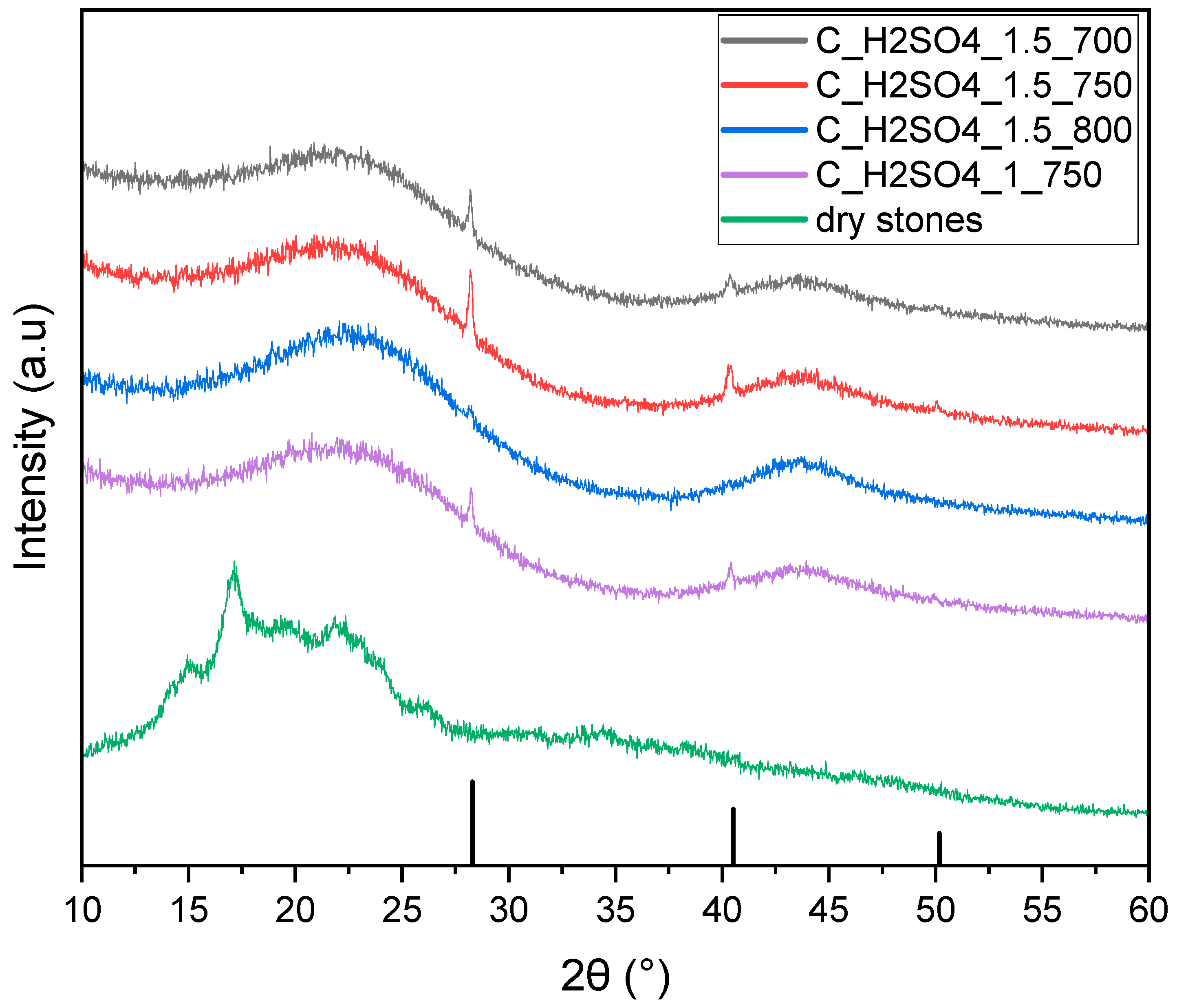
The graphitic structure and the purity of activated carbons were analyzed by the XRD method. Figure 2 shows the XRD patterns of the samples. Two broad peaks cantered at about 2θ = 23 and 43° were observed. The broad peaks indicated a highly disordered carbon structure, which is typical for activated carbons. The observed diffractogram peak positions and their respective widths at half height exhibited remarkable congruence, underlining the similarity of the structure and degree of disorder among the investigated carbon materials.
Two sharp peaks at diffraction angles of 28.3° and 40.5° were observed in the diffraction pattern of all activated carbons. A third small peak was present at 2θ = 50.2° for the C_H2SO4_1.5_750. The peaks were identified as corresponding to KCl (JCPDS 04-0587). Both potassium and chlorine were present in the starting material. KCl peaks were absent on the XRD spectrum of dry seeds. Most likely, KCl crystallization occurred as a result of a series of reactions that occurred during carbonization combined with chemical activation. Based on the different heights of the KCl peaks, it can be assumed that the formation of KCl depends on both the temperature and the amount of sulfuric acid.
The yield of activated carbons depended strongly on the amount of sulfuric acid used (Table 1). At a mass ratio of avocado to acid equal to 1, the yield was 21%. Increasing the amount of acid to 1.5 caused the yield to drop by about half. The temperature of carbonization combined with activation in the range of 700 to 800 °C did not affect the production yield of activated carbon.
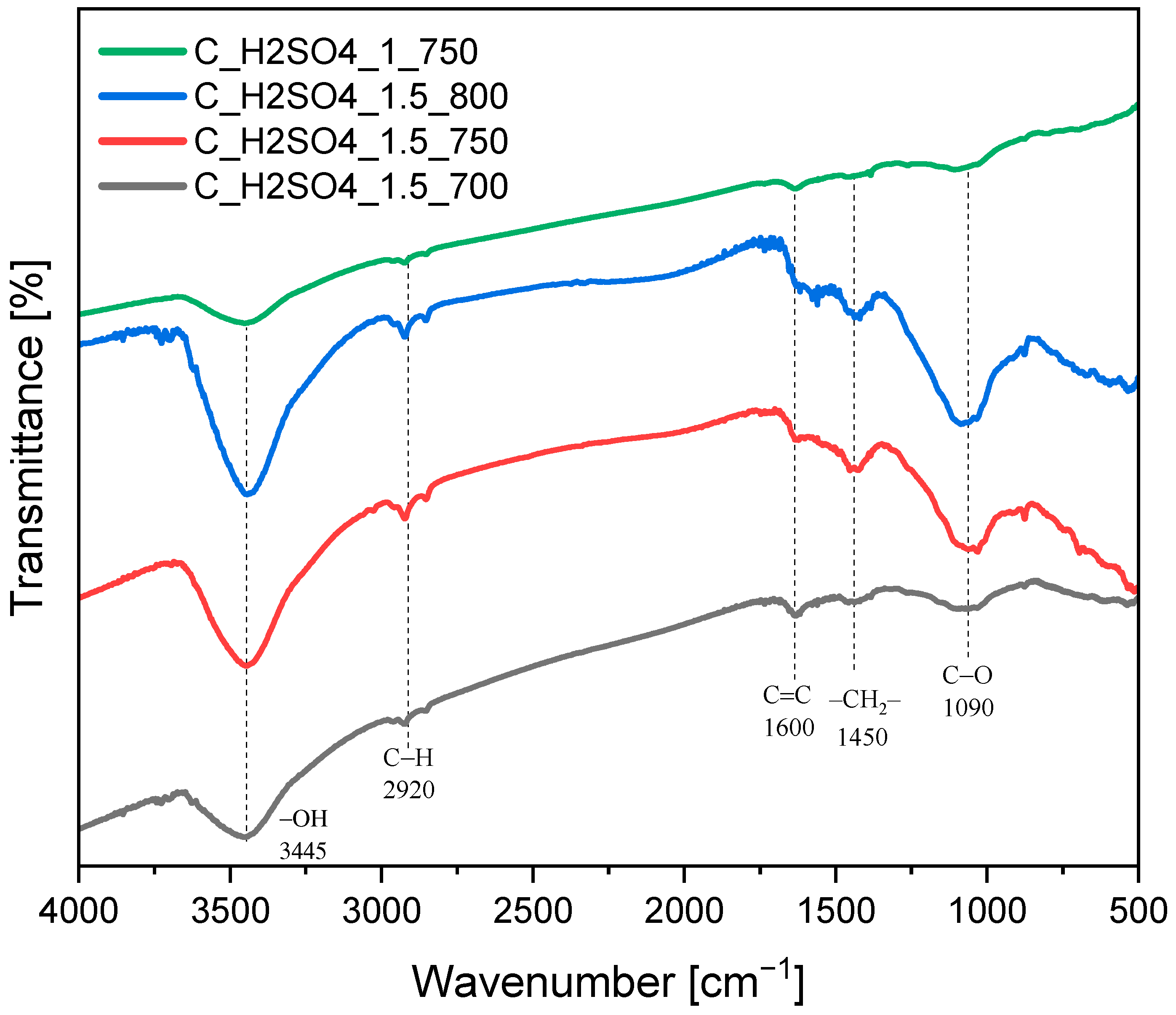
The FTIR spectrum provides valuable insights into the types and amounts of functional groups on the carbon’s surface, which can influence its adsorption properties. Typical functional groups found on activated carbons were observed (Figure 3). The O-H stretching vibrations were observed in the range of 3200–3600 cm−1. Aliphatic C-H stretching vibrations were identified at approximately 2920 cm−1. Carbon–carbon (C-C) bonds, typical for activated carbons, were observed at 1600 cm−1. At 1450 cm−1, stretching vibrations of the CH2 groups were also detected. Bands at 1090 cm−1, associated with C-O stretching vibrations, indicated the presence of various oxygen-containing functional groups, including ethers, alcohols, and phenolic groups.
Polar functional groups on the activated carbon surface, such as hydroxyl (-OH), are crucial for CO2 adsorption. CO2 molecules can form weak chemical bonds (such as hydrogen bonding) with these polar groups, enhancing their adsorption capacity.
Isotherms of nitrogen adsorption at 77 K are depicted in Figure 4. All of the isotherms exhibit a swift rise at low p/p0 pressure values, suggesting that the activated carbons derived from avocado stones and activated by H2SO4 are microporous materials. Notably, hysteresis loops for all samples appear exceedingly narrow, occasionally even imperceptible, without adequate magnification. The presence of these hysteresis loops indicates the coexistence of mesopores alongside the micropores.
All of the nitrogen adsorption isotherms depicted in Figure 1 can be classified as type I according to the IUPAC classification or, more precisely, type Ia [33]. This pattern is indicative of an ordered microporous material. The slight hysteresis loops observed in the examined coals were of the H4 type, which is associated with the presence of slit-like mesopores [34].
The data presented in Table 2 confirm the conclusions drawn from the figure. They indicate the presence of micropores (approximately 80% of all pores) and mesopores. The specific surface area of the adsorbents ranged from 538 to 636 m2/g. The highest surface area, total pore volume, and micropore volume were observed for the material carbonized at the temperature of 750 °C with the ratio of activator to carbon source equal to 1.5 (C_H2SO4_1.5_750). Changes in the carbonization temperature and the ratio of the activator to the carbon source led to a decrease in the textural parameters.
Analyzing the effect of temperature on textural properties, it was found that the highest values for specific surface area, pore volume and micropores were obtained for the average temperature carbonization combined with activation, i.e., 750 °C. A lower temperature (700 °C) was too low for the development of sufficient porosity. At the higher temperature (800 °C), the porous structure that formed was partially degraded. Reducing the amount of activating agent, i.e., sulfuric acid, led to a decrease in the values of textural parameters. Too low an amount of activating agent did not allow sufficient development of the porous structure.
On the basis of values from the Table 3, we can assume that the Rouquerol criteria have been met and the BET equation can be applied for these activated carbons.
Figure 5 shows the pore size distribution determined by the DFT method based on nitrogen adsorption measurements. The method allows for determining the content of pores with diameters in the range of 0.3–30 nm. However, no significant pore volume with diameters larger than 2 nm was observed. Therefore, in Figure 5, on the x-axis, a range up to 3 is presented. The highest pore volume was observed for small micropores in the range of 0.3–0.6 nm.
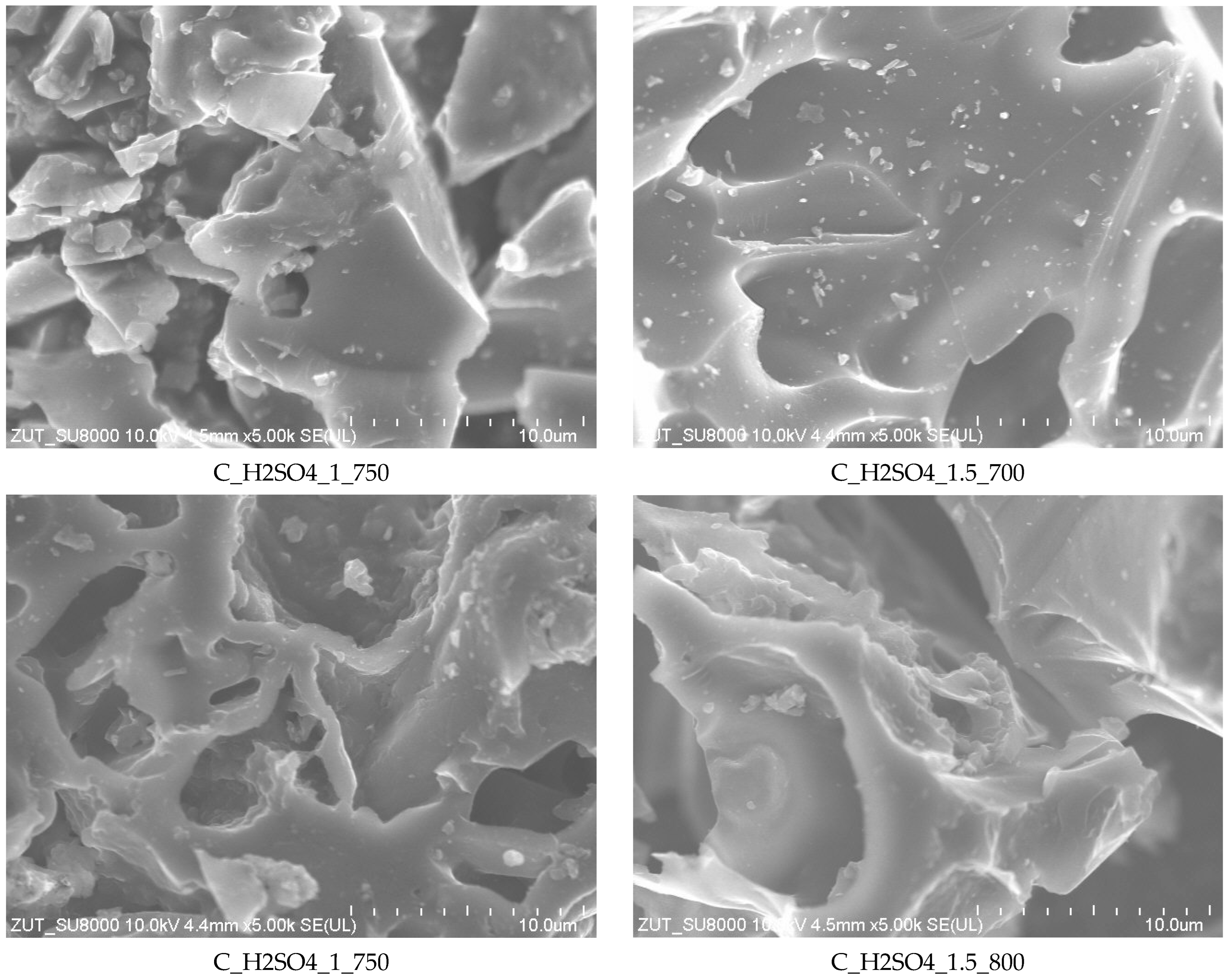
Figure 6 shows SEM images of the obtained activated carbons Their morphology was very similar and significantly different from the starting material. The SEM images show macropores that serve as the initial conduits within porous materials, and they frequently bifurcate into smaller structures known as mesopores. These mesopores, in turn, exhibit a branching pattern, further subdividing into even smaller entities called micropores. This hierarchical arrangement of pores plays a crucial role in determining the material’s overall surface area and its capacity for various adsorption processes.
Activated carbons were tested for their CO2 adsorption capabilities. The experiments were conducted at a temperature of 0 °C and a pressure to 1 bar. The results are depicted in Figure 7. For all of the activated carbons, the CO2 adsorption isotherms at 0 °C exhibited a similar pattern, showing rapid growth at low pressures followed by a more gradual increase at higher pressures. Table 2 lists textural parameters of activated carbons prepared from avocado stones and activated by H2SO4 and CO2 adsorption at a temperature of 0 °C and pressure of 1 bar..
The highest CO2 adsorption, under a pressure of 1 bar, was achieved using activated carbon obtained at a temperature of 750 °C, with a mass ratio of H2SO4 to avocado seed equal to 1.5. The adsorption of carbon dioxide on C_H2SO4_1.5_750 was equal to 3.78 mmol/g.
Table 4 presents a summary of CO2 adsorption outcomes for activated carbons derived from diverse carbon sources. While our CO2 adsorption results may not claim the top position, they remain competitive when juxtaposed with outcomes from alternative materials.
Experimental data of CO2 adsorption isotherms (Figure 7) were analyzed using the Langmuir, Freundlich, Sips, Toth, Radke–Prausnitz, and UNILAN equations. The parameters of these isotherm models were determined through non-linear regression analysis. To assess the quality of the model fit to the experimental data, the following error methods were employed: SSE, SAE, ARE, MPSD, HYBRID and SNE. The detailed results are presented in Table 5, Table 6, Table 7, Table 8, Table 9 and Table 10.
Table 5 displays the Langmuir isotherm constants obtained through non-linear regression for C_H2SO4_1.5_800, C_H2SO4_1.5_750, C_H2SO4_1.5_700, and C_H2SO4_1_750 using different error functions. The derived values of constants qmL and bL for each material are found to exhibit similarity. However, it is noteworthy that the error magnitudes are relatively high. SNE ranged from 3.6664 to 4.6744. This observation indicates that the Langmuir isotherm does not serve as an optimal model for accurately describing carbon dioxide adsorption on carbons activated by H2SO4. In light of the sum of normalized errors (SNE) analysis, it is apparent that the parameter sets yielding the most favorable overall Langmuir fit are based on the ARE. Table 6 presents the Freundlich isotherm constants acquired via non-linear regression for the experimental conditions denoted as C_H2SO4_1.5_800, C_H2SO4_1.5_750, C_H2SO4_1.5_700, and C_H2SO4_1_750. Various error functions were employed during the regression analysis to assess the goodness-of-fit of the model to the experimental data. The determined values of the Freundlich constants, bF and nF, for each studied material, display a degree of similarity. Nevertheless, it is essential to acknowledge that the associated error magnitudes are relatively elevated. The SNE ranges from 3.4679 to 4.4975, which signifies that the Freundlich isotherm model does not provide an optimal fit for precisely characterizing the process of carbon dioxide adsorption on carbons produced from avocado seeds activated by H2SO4. The analysis of SNE reveals that among the investigated parameter sets, the HYBRID approach yields the most favorable overall fit for both C_H2SO4_1.5_750 and C_H2SO4_1.5_800 in the context of the Freundlich isotherm model. On the other hand, for C_H2SO4_1.5_700 and C_H2SO4_1_750, the ARE error function demonstrates superior performance in achieving an optimal fit. These findings suggest that different error functions may be more suitable for specific adsorbent systems, emphasizing the significance of selecting appropriate error metrics tailored to the unique characteristics of the adsorption process under investigation.
Table 7 presents the Sips isotherm constants that were determined through non-linear regression, employing a diverse range of error functions. The derived constants, qmS, bS, and nS, exhibit similarity across all error functions, indicating consistent adsorption behavior across the adsorbents studied. The error magnitudes are relatively low. SNE ranged from 2.7578 to 4.4812. The SNE values for C_H2SO4_1.5_750 and C_H2SO4_1_750 adsorbents are the lowest compared to other models, highlighting the Sips equation’s efficacy in providing a reasonable approximation to the optimum parameter set. The ARE error function provides the most favorable overall fit for both of these materials. For the other two sorbents, the HYBRID error function proves to be more suitable. These results underscore the importance of employing specific error metrics tailored to the characteristics of individual adsorbent systems. Based on the findings, it is recommended to utilize the Sips isotherm equation for the analysis of experimental data for C_H2SO4_1.5_750 and C_H2SO4_1_750 due to its consistently good fit regardless of the chosen error function. This conclusion is corroborated by the excellent agreement between the experimental adsorption isotherm and the Sips equation model, further supporting the suitability of the Sips model for describing the adsorption process in the study of these materials.
Table 8 presents the Toth isotherm constants obtained through non-linear regression for C_H2SO4_1.5_800, C_H2SO4_1.5_750, C_H2SO4_1.5_700, and C_H2SO4_1_750, employing different error functions. The derived values of qmT, bT and nT for each material show a degree of similarity. However, it is important to note that the associated error magnitudes are the highest, with SNE values ranging from 3.8325 to4.7586. This finding suggests that the Toth isotherm model is the least suitable for accurately describing carbon dioxide adsorption on carbons activated by H2SO4. The analysis of SNE indicates that the parameter sets yielding the most favorable overall Toth fit are based on the HYBRID.
Table 9 presents the Radke–Prausnitz isotherm constants obtained through non-linear regression for activated carbons produced from avocado stones activated by H2SO4, utilizing different error functions. Each material exhibits a noticeable degree of similarity in the determined values of constants qmRP, bRP and nRP. However, it is pertinent to acknowledge that the associated error magnitudes are relatively low, with SNE values ranging from 3.1571 to 4.2494. These findings collectively indicate that the Radke–Prausnitz isotherm model does not serve as an optimal representation for accurately describing carbon dioxide adsorption on carbons activated by H2SO4. The observed high SNE values suggest that the model does not adequately capture the complexity of the adsorption process under investigation. In light of the SNE analysis, it becomes evident that the parameter sets leading to the most favorable overall Radke–Prausnitz fit are those based on the ARE.
Table 10 presents the UNILAN isotherm constants determined through non-linear regression, employing a diverse range of error functions. The derived constants, qmU, bU, and s, demonstrate a remarkable degree of similarity across all error functions, indicating consistent adsorption behavior across the studied adsorbents. It is noteworthy that the error magnitudes associated with the UNILAN model are relatively low, with SNE values ranging from 3.0383 to 4.6702. Particularly, for the C_H2SO4_1.5_700 and C_H2SO4_1_750 adsorbents, the SNE values are the lowest compared to other models, highlighting the UNILAN equation’s efficacy in providing a reasonable approximation to the optimum parameter set. The analysis reveals that the ARE error function yields the most favorable overall fit for both the C_H2SO4_1.5_750 and C_H2SO4_1.5_800 materials. Conversely, for the other two sorbents (C_H2SO4_1.5_700 and C_H2SO4_1.5_700), the SSE error function demonstrates greater suitability. Based on these findings, it is recommended to employ the UNILAN isotherm equation for the analysis of experimental data concerning the _H2SO4_1.5_700 and C_H2SO4_1_750 materials due to its consistent good fit regardless of the chosen error function. This conclusion is further supported by the excellent agreement between the experimental adsorption isotherm and the UNILAN equation model, reaffirming the suitability of the Sips model for accurately describing the adsorption process in the study of these materials.
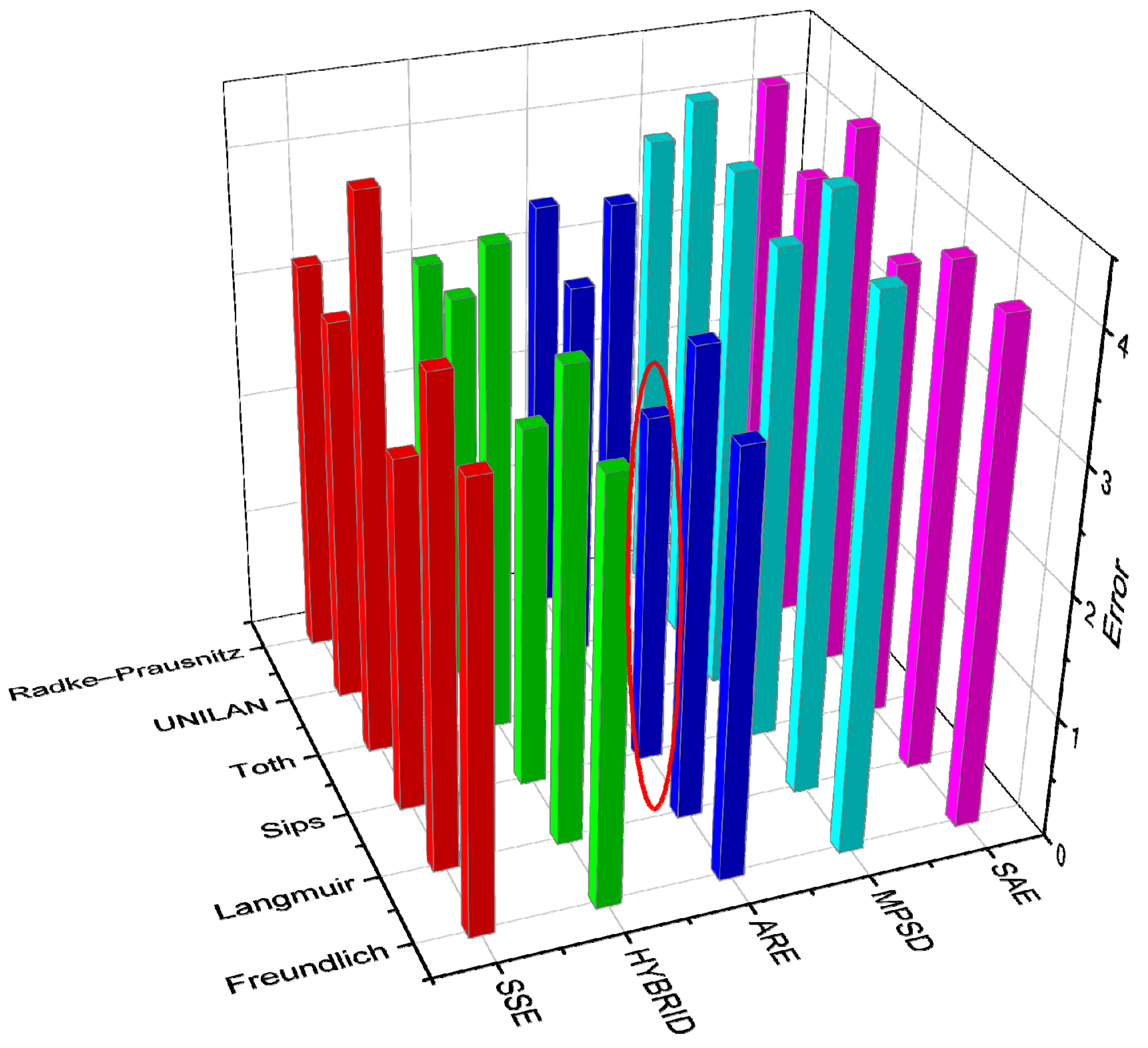
Figure 8 shows the analysis of adsorption isotherms and the error function used for the calculations of the best CO2 sorbent, i.e., C_H2SO4_1.5_750.
It was found that the Sips equation described the adsorption data in the best way. The most appropriate error function was ARE.
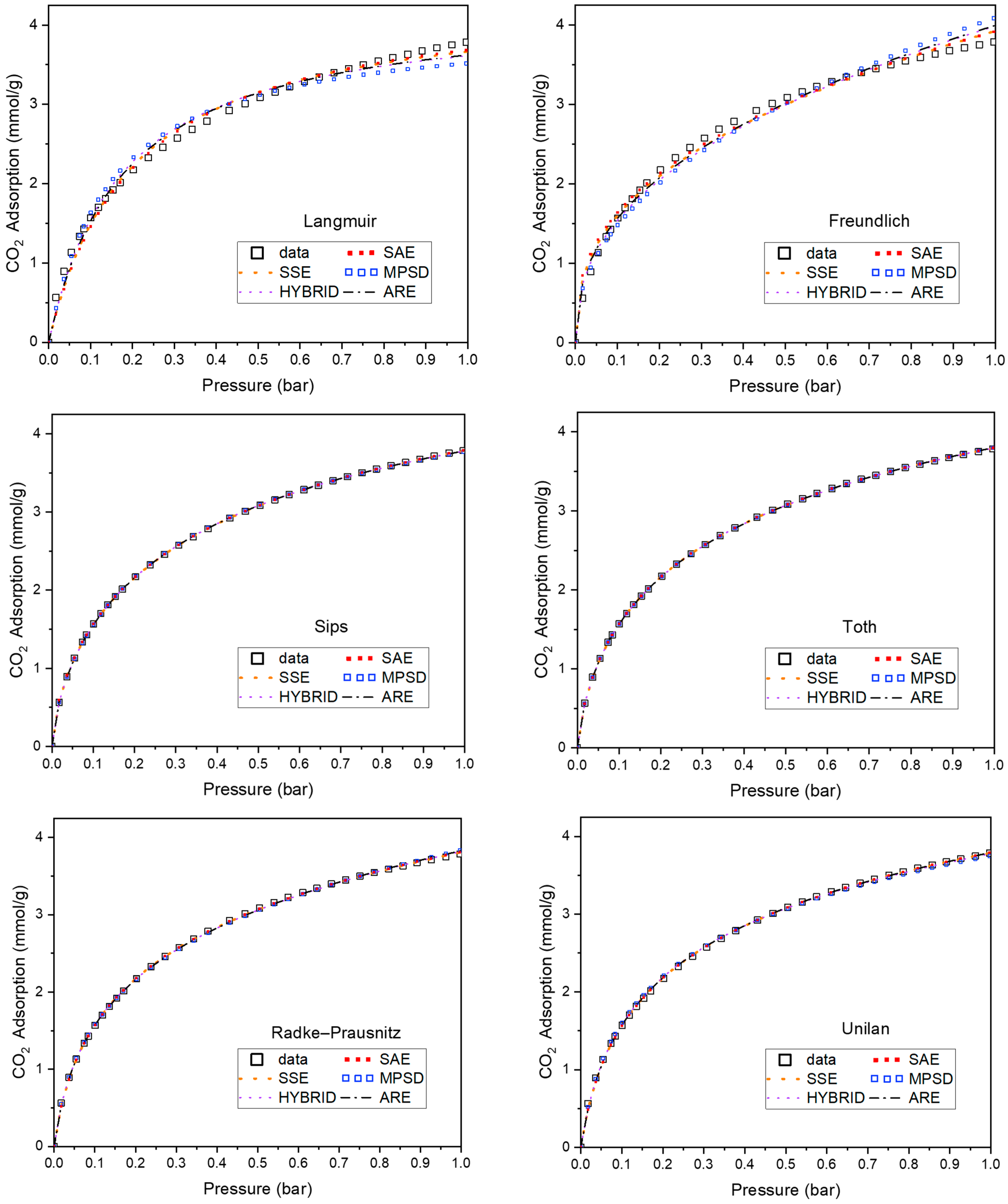
Figure 9 presents the results of model fitting for CO2 adsorption on C_H2SO4_1.5_750 at 0 °C using different error functions for the following models: Langmuir, Freundlich, Sips, Toth, Radke–Prausnitz, and UNILAN. It is evident that the Langmuir and Freundlich models are significantly inferior, while the Sips model performs the best.
The CO2 adsorption investigations over C_H2SO4_1.5_750 at higher temperatures i.e., 10, 20, and 30 °C, were performed (Figure 10). An increase in the CO2 adsorption temperature leads to a decrease in CO2 adsorption, indicating the physical nature of CO2 adsorption on C_H2SO4_1.5_750.
It was found that the adsorption data presented in Figure 10 can be described by the Sips equation.
The Sips model coefficients for different temperatures for C_H2SO4_1.5_750 are presented in Table 11. The maximum adsorption value (qmS) decreases with an increase in temperature. This also confirms the physical nature of CO2 adsorption over C_H2SO4_1.5_750.
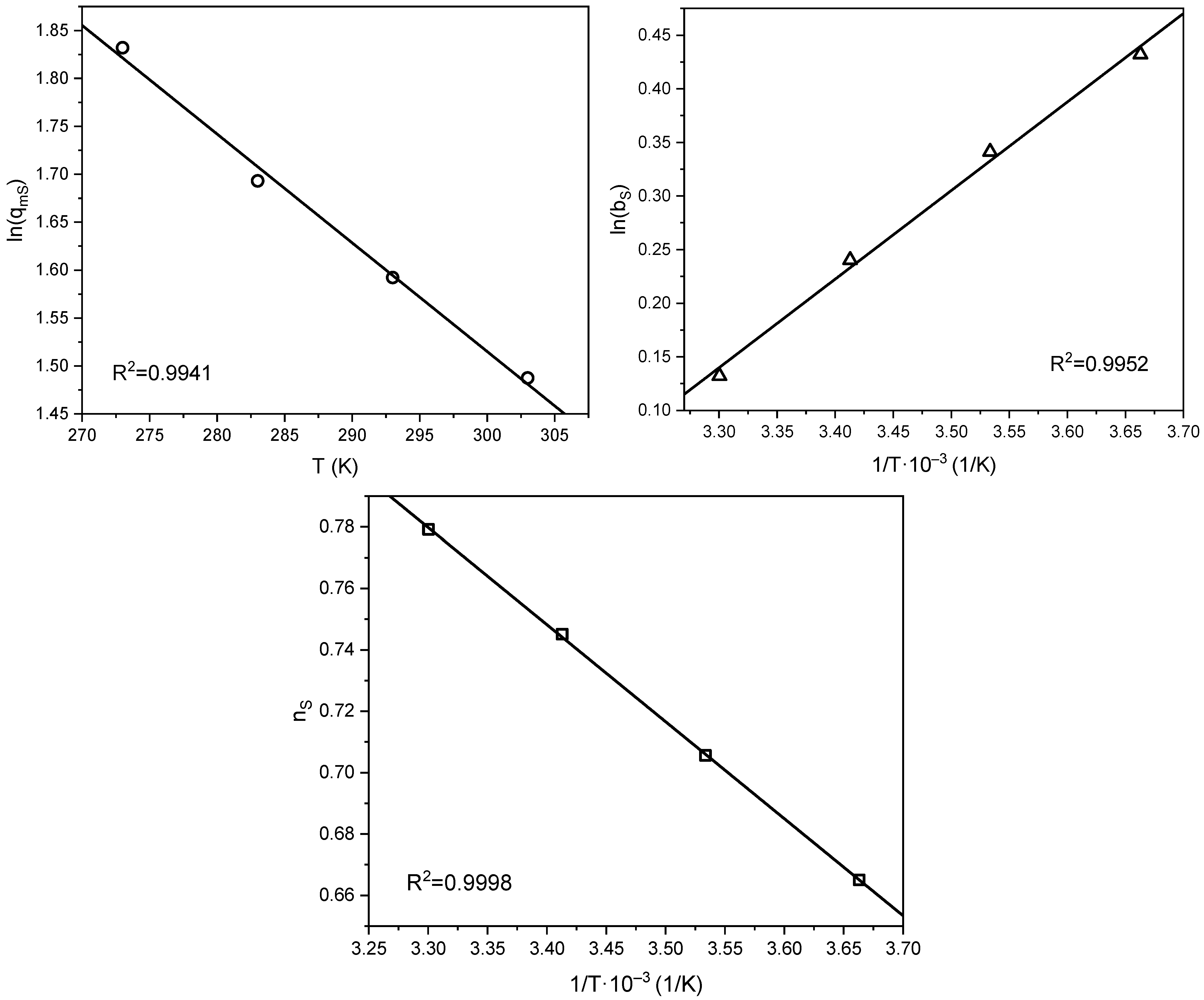
The coefficients within the Sips Equation (4) exhibit temperature dependency described by Equations (15)–(17):
q m S = q m 0 · e x p χ 1 T T 0
b S = b 0 e x p Q R T T 0 T 1
n S = n 0 + α 1 T 0 T
By plotting ln(qmS) vs. T, ln(bS) vs. 1/T and nS vs. 1/T, linear functions are supposed to be obtained.
The functions depicted in Figure 11 exhibit a linear course. R-squared for each function yielded a value greater than 0.99. This confirms that the Sips equation accurately describes CO2 adsorption, not only at 0 °C but also within the temperature range of 0 °C to 30°.
The value of the isosteric heat of adsorption (Qiso) is essential for characterizing the interactions between the adsorbent and the adsorbate, providing information on the adsorption strength. A higher Q
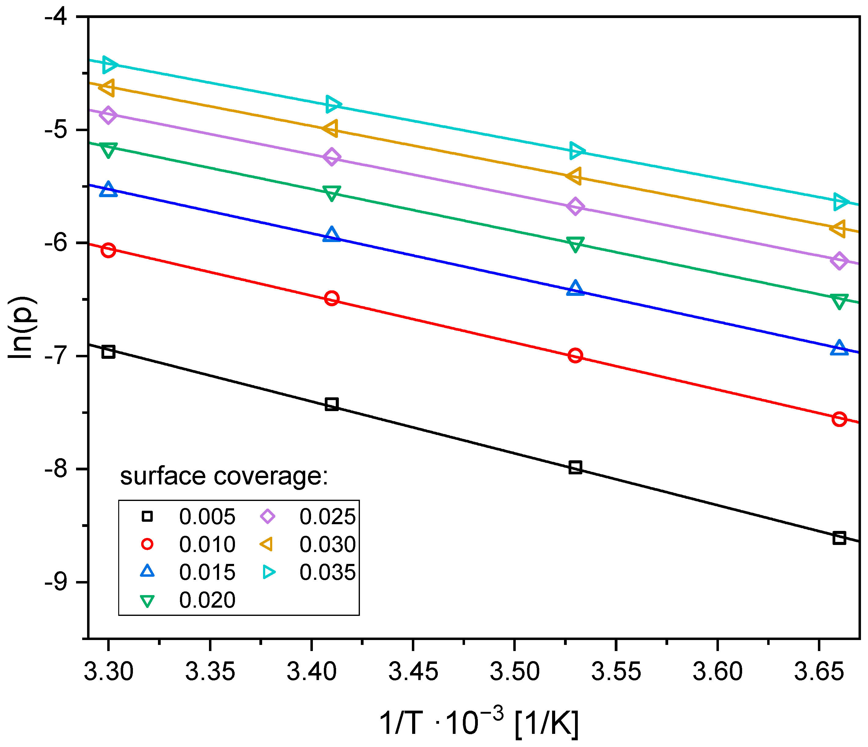
iso value indicates a stronger interaction between the adsorbate and the adsorbent. However, it also results in a higher cost of regeneration. The isosteric heat of adsorption was calculated using Equation (14). To determine the pressure values for a given degree of surface coverage, the Sips Equation (4) was transformed appropriately (18).
p = θ b S θ · b S 1 n S
where θ, the degree of surface coverage, is defined as (19):
θ = q q m S
Parameter values in the Sips equation (qmS, bS, nS) are derived from Table 11. Isosteric graphs, i.e., the relationship between ln(p)θ and 1/T for temperatures in the range of 0–30 °C are presented in Figure 12. On the basis of the values of the slope coefficients of the drawn straight lines, the values of the isosteric heat of adsorption for C_H2SO4_1.5_750 were calculated depending on the degree of coverage (14).
The values of the isosteric heat of CO2 adsorption for C_H2SO4_1.5_750 as a function of the degree of surface coverage are shown in Figure 13.
The values of isosteric heat ranged from 28 to 38 kJ/mol for surface coverages from 0.035 to 0.005. These values definitely confirm the physical nature of CO2 sorption on activated carbons. The isosteric heat of adsorption decreased with surface coverage. The greater the surface coverage, the weaker the interaction between carbon dioxide and activated carbons. Carbon dioxide is bound to the surface of activated carbons by van der Waals forces and can be easily desorbed. The isosteric heat of CO2 adsorption on the tested material was low, which makes C_H2SO4_1.5_750 a potentially useful CO2 sorbent.

5. Conclusions

The influence of the temperature of carbonization combined with chemical activation and the amount of activating agent on the porosity of activated carbon derived from avocado stones, activated by H2SO4 and CO2 adsorption, is noteworthy. To achieve the production of adsorbents suitable for CO2 capture, a judicious choice of carbonization combined with chemical activation temperature and amount of H2SO4 is crucial. Notably, a relatively moderate temperature of 750 °C and mass ratio of H2SO4: dry avocado stones proves essential.
The investigation demonstrated the significant impact of both the isotherm type selection and the employed error function for parameter extraction on the predictive efficacy of the models. The adsorption equilibrium of CO2 on activated carbons derived from avocado stones through sulfuric acid activation lends itself well to accurate description using the Sips and UNILAN equations. In pursuit of precise calculations, the adoption of the ARE and HYBRID error functions is recommended for optimal model performance.

Author Contributions

Conceptualization, J.S. and B.M.; methodology, J.S. and B.M.; investigation, J.S.; data curation, J.S.; writing—original draft preparation, J.S. and B.M.; writing—review and editing, J.S. and B.M.; visualization, J.S.; supervision, B.M. All authors have read and agreed to the published version of the manuscript.

Funding

This research received no external funding.

Institutional Review Board Statement

Not applicable.

Informed Consent Statement

Not applicable.

Data Availability Statement

The data presented in this study are available upon request from the corresponding author.

Conflicts of Interest

The authors declare no conflict of interest.

References

  1. Hussin, F.; Hazani, N.N.; Aroua, M.K. The Effect of Physicochemical Properties and Surface Chemistry on CO2 Adsorption Capacity of Potassium Acetate-Treated Carbon Pellets. Sustainability 2023, 15, 4903. [Google Scholar] [CrossRef]
  2. Daily CO2. Available online: https://www.Co2.Earth/Daily-Co2 (accessed on 27 July 2023).
  3. Li, S.; Jia, S.; Nagasaka, T.; Bai, H.; Yang, L. CO2 Adsorption Properties of Amine-Modified Zeolites Synthesized Using Different Types of Solid Waste. Sustainability 2023, 15, 10144. [Google Scholar] [CrossRef]
  4. Kiełbasa, K. Activated Biocarbons Derived from Molasses as New Tailored CO2 Adsorbents. Front. Chem. 2023, 11, 1184389. [Google Scholar] [CrossRef] [PubMed]
  5. Gan, Y.X. Activated Carbon from Biomass Sustainable Sources. J. Carbon Res. C 2021, 7, 39. [Google Scholar] [CrossRef]
  6. Kim, K.H.; Kim, M.H. Adsorption of CO2, CO, H2, and N2 on Zeolites, Activated Carbons, and Metal-Organic Frameworks with Different Surface Nonuniformities. Sustainability 2023, 15, 11574. [Google Scholar] [CrossRef]
  7. Jahanban-Esfahlan, A.; Jahanban-Esfahlan, R.; Tabibiazar, M.; Roufegarinejad, L.; Amarowicz, R. Recent Advances in the Use of Walnut (Juglans regia L.) Shell as a Valuable Plant-Based Bio-Sorbent for the Removal of Hazardous Materials. RSC Adv. 2020, 10, 7026–7047. [Google Scholar] [CrossRef] [PubMed]
  8. Yuan, X.; Wang, Q.; Wang, Z.; Wu, S.; Zhai, Y.; Zhang, H.; Zhou, L.; Lu, B.; Chen, K.; Wang, X. Optimization of Mixed-Based Biochar Preparation Process and Adsorption Performance of Lead and Cadmium. Sustainability 2023, 15, 11579. [Google Scholar] [CrossRef]
  9. Kamińska, A.; Miądlicki, P.; Kiełbasa, K.; Kujbida, M.; Sreńscek-Nazzal, J.; Wróbel, R.J.; Wróblewska, A. Activated Carbons Obtained from Orange Peels, Coffee Grounds, and Sunflower Husks—Comparison of Physicochemical Properties and Activity in the Alpha-Pinene Isomerization Process. Materials 2021, 14, 7448. [Google Scholar] [CrossRef]
  10. Kamińska, A.; Sreńscek-Nazzal, J.; Kiełbasa, K.; Grzeszczak, J.; Serafin, J.; Wróblewska, A. Carbon-Supported Nickel Catalysts—Comparison in Alpha-Pinene Oxidation Activity. Sustainability 2023, 15, 5317. [Google Scholar] [CrossRef]
  11. Kamińska, A.; Miądlicki, P.; Kiełbasa, K.; Serafin, J.; Sreńscek-Nazzal, J.; Wróbel, R.J.; Wróblewska, A. FeCl3-Modified Carbonaceous Catalysts from Orange Peel for Solvent-Free Alpha-Pinene Oxidation. Materials 2021, 14, 7729. [Google Scholar] [CrossRef]
  12. Ariharan, A.; Kim, S.-K. Three-Dimensional Hierarchical Porous Carbons Derived from Betelnut Shells for Supercapacitor Electrodes. Materials 2021, 14, 7793. [Google Scholar] [CrossRef] [PubMed]
  13. Pu, J.; Wang, L.; Huang, J.; Chen, Q.; Jin, Y.; Chen, J. High-Performance Supercapacitors Based on Porous Activated Carbon Derived from Carbon Dots by Directly Pyrolyzing Industrial Glucose. Diam. Relat. Mater. 2023, 132, 109684. [Google Scholar] [CrossRef]
  14. Domínguez, M.P.; Araus, K.; Bonert, P.; Sánchez, F.; San Miguel, G.; Toledo, M. The Avocado and Its Waste: An Approach of Fuel Potential/Application. In Environment, Energy and Climate Change II; Springer: Berlin/Heidelberg, Germany, 2014; pp. 199–223. [Google Scholar]
  15. Perea-Moreno, A.-J.; Aguilera-Ureña, M.-J.; Manzano-Agugliaro, F. Fuel Properties of Avocado Stone. Fuel 2016, 186, 358–364. [Google Scholar] [CrossRef]
  16. Rodrigues, L.A.; da Silva, M.L.C.P.; Alvarez-Mendes, M.O.; dos Reis Coutinho, A.; Thim, G.P. Phenol Removal from Aqueous Solution by Activated Carbon Produced from Avocado Kernel Seeds. Chem. Eng. J. 2011, 174, 49–57. [Google Scholar] [CrossRef]
  17. Leite, A.J.B.; Carmalin, S.A.; Thue, P.S.; dos Reis, G.S.; Dias, S.L.; Lima, E.C.; Vaghetti, J.C.P.; Pavan, F.A.; de Alencar, W.S. Activated Carbon from Avocado Seeds for the Removal of Phenolic Compounds from Aqueous Solutions. Desalin. Water Treat. 2017, 71, 168–181. [Google Scholar] [CrossRef]
  18. Elizalde-González, M.P.; Mattusch, J.; Peláez-Cid, A.A.; Wennrich, R. Characterization of Adsorbent Materials Prepared from Avocado Kernel Seeds: Natural, Activated and Carbonized Forms. J. Anal. Appl. Pyrolysis 2007, 78, 185–193. [Google Scholar] [CrossRef]
  19. Salomón-Negrete, M.Á.; Reynel-Ávila, H.E.; Mendoza-Castillo, D.I.; Bonilla-Petriciolet, A.; Duran-Valle, C.J. Water Defluoridation with Avocado-Based Adsorbents: Synthesis, Physicochemical Characterization and Thermodynamic Studies. J. Mol. Liq. 2018, 254, 188–197. [Google Scholar] [CrossRef]
  20. Bhaumik, M.; Choi, H.J.; Seopela, M.P.; McCrindle, R.I.; Maity, A. Highly Effective Removal of Toxic Cr(VI) from Wastewater Using Sulfuric Acid-Modified Avocado Seed. Ind. Eng. Chem. Res. 2014, 53, 1214–1224. [Google Scholar] [CrossRef]
  21. Kiełbasa, K.; Kamińska, A.; Niedoba, O.; Michalkiewicz, B. CO2 Adsorption on Activated Carbons Prepared from Molasses: A Comparison of Two and Three Parametric Models. Materials 2021, 14, 7458. [Google Scholar] [CrossRef]
  22. Kiełbasa, K.; Bayar, Ş.; Varol, E.A.; Sreńscek-Nazzal, J.; Bosacka, M.; Michalkiewicz, B. Thermochemical Conversion of Lignocellulosic Biomass—Olive Pomace—Into Activated Biocarbon for CO2 Adsorption. Ind. Crops Prod. 2022, 187, 115416. [Google Scholar] [CrossRef]
  23. Rouquerol, F.; Rouquerol, J.; Sing, K. Adsorption by Powders and Porous Solids; Springer: Berlin/Heidelberg, Germany, 1999. [Google Scholar] [CrossRef]
  24. Rouquerol, J.; Llewellyn, P.; Rouquerol, F. Is the Bet Equation Applicable to Microporous Adsorbents? In Studies in Surface Science and Catalysis; Springer: Berlin/Heidelberg, Germany, 2007; pp. 49–56. [Google Scholar]
  25. Kaneko, K.; Ishii, C. Superhigh Surface Area Determination of Microporous Solids. Colloids Surf. 1992, 67, 203–212. [Google Scholar] [CrossRef]
  26. Walton, K.S.; Snurr, R.Q. Applicability of the BET Method for Determining Surface Areas of Microporous Metal−Organic Frameworks. J. Am. Chem. Soc. 2007, 129, 8552–8556. [Google Scholar] [CrossRef] [PubMed]
  27. Ayawei, N.; Angaye, S.S.; Wankasi, D.; Dikio, E.D. Synthesis, Characterization and Application of Mg/Al Layered Double Hydroxide for the Degradation of Congo Red in Aqueous Solution. Open J. Phys. Chem. 2015, 05, 56–70. [Google Scholar] [CrossRef]
  28. Ning, P.; Li, F.; Yi, H.; Tang, X.; Peng, J.; Li, Y.; He, D.; Deng, H. Adsorption Equilibrium of Methane and Carbon Dioxide on Microwave-Activated Carbon. Sep. Purif. Technol. 2012, 98, 321–326. [Google Scholar] [CrossRef]
  29. Toth, J. State Equations of Solid-Gas Interface Layers. Acta Chim. Acad. Sci. Hung. 1971, 69, 311–328. [Google Scholar]
  30. Radke, C.J.; Prausnitz, J.M. Thermodynamics of Multi-Solute Adsorption from Dilute Liquid Solutions. AIChE J. 1972, 18, 761–768. [Google Scholar] [CrossRef]
  31. Do, D.D. Adsorption Analysis: Equilibria and Kinetics; Imperial College Press: London, UK, 1998; Volume 2, ISBN 1860941303. [Google Scholar]
  32. Porter, J.F.; McKay, G.; Choy, K.H. The Prediction of Sorption from a Binary Mixture of Acidic Dyes Using Single- and Mixed-Isotherm Variants of the Ideal Adsorbed Solute Theory. Chem. Eng. Sci. 1999, 54, 5863–5885. [Google Scholar] [CrossRef]
  33. Thommes, M.; Kaneko, K.; Neimark, A.V.; Olivier, J.P.; Rodriguez-Reinoso, F.; Rouquerol, J.; Sing, K.S.W. Physisorption of Gases, with Special Reference to the Evaluation of Surface Area and Pore Size Distribution (IUPAC Technical Report). Pure Appl. Chem. 2015, 87, 1051–1069. [Google Scholar] [CrossRef]
  34. Sing, K.S.W. Reporting Physisorption Data for Gas/Solid Systems with Special Reference to the Determination of Surface Area and Porosity (Recommendations 1984). Pure Appl. Chem. 1985, 57, 603–619. [Google Scholar] [CrossRef]
  35. Yuan, B.; Wu, X.; Chen, Y.; Huang, J.; Luo, H.; Deng, S. Adsorption of CO2, CH4, and N2 on Ordered Mesoporous Carbon: Approach for Greenhouse Gases Capture and Biogas Upgrading. Environ. Sci. Technol. 2013, 47, 5474–5480. [Google Scholar] [CrossRef]
  36. Choma, J.; Marszewski, M.; Osuchowski, L.; Jagiello, J.; Dziura, A.; Jaroniec, M. Adsorption Properties of Activated Carbons Prepared from Waste CDs and DVDs. ACS Sustain. Chem. Eng. 2015, 3, 733–742. [Google Scholar] [CrossRef]
  37. Makhseed, S.; Samuel, J. Imide-Linked Microporous Organic Framework Polymers for CO2 Adsorption. Polymer 2015, 74, 144–149. [Google Scholar] [CrossRef]
  38. Serafin, J.; Sreńscek-Nazzal, J.; Kamińska, A.; Paszkiewicz, O.; Michalkiewicz, B. Management of Surgical Mask Waste to Activated Carbons for CO2 Capture. J. CO2 Util. 2022, 59, 101970. [Google Scholar] [CrossRef] [PubMed]
  39. Huang, G.; Liu, Y.; Wu, X.; Cai, J. Activated Carbons Prepared by the KOH Activation of a Hydrochar from Garlic Peel and Their CO2 Adsorption Performance. New Carbon Mater. 2019, 34, 247–257. [Google Scholar] [CrossRef]
  40. Serafin, J.; Ouzzine, M.; Cruz, O.F.; Sreńscek-Nazzal, J.; Campello Gómez, I.; Azar, F.-Z.; Rey Mafull, C.A.; Hotza, D.; Rambo, C.R. Conversion of Fruit Waste-Derived Biomass to Highly Microporous Activated Carbon for Enhanced CO2 Capture. Waste Manag. 2021, 136, 273–282. [Google Scholar] [CrossRef]
Figure 1. SEM picture of dry avocado seed particle.
Sustainability 15 16881 g001
Figure 2. XRD patterns of activated carbons prepared from avocado stones and activated by H2SO4. Black bars indicate KCl patterns according to JCPDS 04-0587.
Sustainability 15 16881 g002
Figure 3. FTIR study of activated carbons prepared from avocado stones and activated by H2SO4.
Sustainability 15 16881 g003
Figure 4. N2 adsorption−desorption isotherms on activated carbons prepared from avocado stones and activated by H2SO4.
Sustainability 15 16881 g004
Figure 5. Pore size distribution of activated carbons, prepared from avocado stones and activated by H2SO4, determined using the DFT method based on N2 sorption at a temperature of 77 K.
Sustainability 15 16881 g005
Figure 6. SEM pictures of activated carbons prepared from avocado stones and activated by H2SO4.
Sustainability 15 16881 g006
Figure 7. CO2 adsorption isotherms over activated carbons prepared from avocado stones and activated by H2SO4.
Sustainability 15 16881 g007
Figure 8. Analysis of adsorption isotherms and the error function used for C_H2SO4_1.5_750. The best result is marked by red circle. Bars: red: SSE, green: HYBRID, marina: ARE, blue: MPSD, magenta: SAE.
Sustainability 15 16881 g008
Figure 9. CO2 adsorption data at temperature 0 °C for C_H2SO4_1.5_750 and fitting curves for different models and error functions.
Sustainability 15 16881 g009
Figure 10. The CO2 adsorption over C_H2SO4_1.5_750 at different temperatures.
Sustainability 15 16881 g010
Figure 11. Set of plots for ln(qmS) vs. T, bS vs. 1/T, and nS vs. 1/T according to Equations (15)–(17). Points on the basis on the Table 11.
Sustainability 15 16881 g011
Figure 12. Adsorption isosteres with different surface coverage on C_H2SO4_1.5_750.
Sustainability 15 16881 g012
Figure 13. Isosteric heat of CO2 adsorption for C_H2SO4_1.5_750 at different degrees of surface coverage. Points were calculated on the basis of Figure 12.
Sustainability 15 16881 g013
Table 1. The yield of activated carbons prepared from avocado stones and activated by H2SO4.
ACYield
C_H2SO4_1_75021%
C_H2SO4_1.5_70010%
C_H2SO4_1.5_75010%
C_H2SO4_1.5_80011%
Table 2. Textural parameters of activated carbons prepared from avocado stones and activated by H2SO4 and CO2 adsorption at a temperature of 0 °C and pressure of 1 bar.
ACSSAVtotVmicqCO2
(m2·g−1)(cm3·g−1)(cm3·g−1)(mmol·g−1)
C_H2SO4_1_7505380.2170.1753.34
C_H2SO4_1.5_7005960.2480.1983.64
C_H2SO4_1.5_7506360.2580.2093.78
C_H2SO4_1.5_8005660.2360.1883.64
Table 3. The relative pressure range for linear BET region (RPR), constant that characterizes the strength of the adsorption energy (C), monolayer capacity (nm) and standard deviation (R2).
ACRPRCtnmR2
C_H2SO4_1_7501.17 × 10−7–0.057412,0960.02460.99996
C_H2SO4_1.5_7001.10 × 10−7–0.072264,3340.02710.99997
C_H2SO4_1.5_7501.03 × 10−7–0.063351,1180.02910.99999
C_H2SO4_1.5_8000.98 × 10−7–0.070913,5990.02590.99997
Table 4. CO2 adsorption of various carbons at 1 bar and 0 °C.
ACqCO2Ref.
(mmol·g−1)
ordered mesoporous carbon3.0[35]
AC from waste CDs4.3[36]
organic framework polymers with intrinsic microporosity2.9[37]
AC from mask waste3.9[38]
AC from garlic peel4.33[39]
AC from polypodium vulgare9.09[40]
C_H2SO4_1.5_7503.78this work
Table 5. Langmuir isotherm constants with error analysis.
SSEHYBRIDAREMPSDSAE
C_H2SO4_1.5_700
qmL4.13964.01084.05993.83114.1961
bL5.69336.41516.02247.50655.3437
SSE0.28740.33980.30490.58830.3047
HYBRID0.70490.61370.64810.77100.8399
ARE4.67704.60784.55845.12714.9540
MPSD8.72327.41228.11766.73139.6840
SAE2.57872.94542.70253.82492.5258
SNE3.81503.74243.72394.61304.1445
C_H2SO4_1.5_750
qmL4.37614.23794.27204.03874.4430
bL5.15785.78255.57776.75954.8530
SSE0.28180.33420.30810.59680.2975
HYBRID0.68540.59720.60810.76050.8117
ARE4.63004.50154.47105.03614.8816
MPSD8.64847.38637.75756.70419.5468
SAE2.56632.90182.75253.83112.4999
SNE3.81163.72063.68424.63914.1204
C_H2SO4_1.5_800
qmL4.22614.07854.10713.86514.2842
bL5.00345.66745.48536.73374.7188
SSE0.30420.36080.33720.65140.3189
HYBRID0.77960.68120.69010.86910.9056
ARE5.04494.91994.88475.46715.2696
MPSD9.43938.09968.42727.364610.3045
SAE2.65983.01152.88023.97262.5874
SNE3.83633.75003.71604.67444.1047
C_H2SO4_1_750
qmL3.79313.67633.69483.50903.8629
bL5.71756.42886.17637.53585.3040
SSE0.23180.27480.25850.48630.2501
HYBRID0.63100.55030.57000.69710.7743
ARE4.61544.51894.49395.11724.9303
MPSD8.68577.40837.87696.72219.7761
SAE2.30662.62942.49663.49262.2464
SNE3.74253.66963.66644.58794.1209
Table 6. Freundlich isotherm constants with error analysis.
SSEHYBRIDAREMPSDSAE
C_H2SO4_1.5_700
bF3.77653.83573.83643.92833.7565
nF0.37460.39830.38910.42540.3600
SSE0.26410.32890.29990.57110.2938
HYBRID0.70440.57170.60750.72720.9528
ARE4.46454.35154.28194.88744.8673
MPSD9.23087.16118.00236.298511.0834
SAE2.41382.85592.62213.70922.3049
SNE3.59893.48243.46794.33164.1318
C_H2SO4_1.5_750
bF3.92353.98603.99374.08863.9169
nF0.38940.41360.40690.44230.3799
SSE0.27010.33960.31960.61650.2857
HYBRID0.71790.57920.60530.75490.8756
ARE4.49104.32074.27244.94724.7541
MPSD9.47947.33207.98136.390210.7176
SAE2.46072.89092.71883.85392.3777
SNE3.68883.52003.52354.45844.0414
C_H2SO4_1.5_800
bF3.76873.82363.83063.91483.7615
nF0.39400.41600.40920.44230.3862
SSE0.20330.25560.24010.46770.2119
HYBRID0.56360.45530.48050.59520.6687
ARE4.03033.91953.85274.50424.2587
MPSD8.59346.66377.32505.80949.5646
SAE2.11312.51132.33723.35912.0615
SNE3.69973.54183.54904.49754.0123
C_H2SO4_1_750
bF3.46183.51853.51963.60853.4509
nF0.37250.39690.38810.42530.3611
SSE0.23440.29290.26790.51660.2516
HYBRID0.68530.55550.58700.71260.8643
ARE4.59724.47404.41445.10234.9046
MPSD9.57967.42458.24446.505811.0579
SAE2.28542.70102.49633.56282.1966
SNE3.65553.51603.50914.41294.0647
Table 7. Sips isotherm constants with error analysis.
SSEHYBRIDAREMPSDSAE
C_H2SO4_1.5_700
qmS5.77115.65375.66685.53685.8528
bS1.70871.80131.78771.90111.6489
nS0.66430.67540.67260.68570.6557
SSE0.00150.00190.00190.00310.0018
HYBRID0.00420.00330.00350.00400.0067
ARE0.32620.33280.32810.35830.3492
MPSD0.72060.52080.58910.45690.9819
SAE0.17650.22040.21150.27500.1608
SNE3.40163.36073.41434.06994.1441
C_H2SO4_1.5_750
qmS6.12936.00966.03065.87606.2464
bS1.61421.69511.68031.79281.5405
nS0.67580.68600.68440.69670.6650
SSE0.00090.00120.00110.00250.0012
HYBRID0.00340.00260.00260.00350.0065
ARE0.25760.27740.26830.34700.2754
MPSD0.71930.52560.54550.45281.0411
SAE0.11600.16760.15510.25180.0861
SNE2.76342.85042.75783.96693.6432
C_H2SO4_1.5_800
qmS6.28786.15866.24836.00606.3468
bS1.38111.44801.40031.53361.3521
nS0.65100.66010.65410.67030.6471
SSE0.00090.00110.00100.00220.0009
HYBRID0.00330.00270.00300.00350.0039
ARE0.26820.28310.26570.35230.2693
MPSD0.70230.53630.62600.47030.7842
SAE0.11950.15950.12580.23630.1095
SNE3.41113.36583.28494.48123.6600
C_H2SO4_1_750
qmS5.20725.12115.13325.02665.2675
bS1.78081.86041.84811.95351.7277
nS0.67100.68030.67880.68980.6640
SSE0.00060.00080.00080.00170.0008
HYBRID0.00260.00200.00210.00260.0040
ARE0.24040.26020.25010.31670.2425
MPSD0.64770.47830.49950.41780.8331
SAE0.10150.14240.13350.20500.0793
SNE3.07093.11243.03234.16453.6060
Table 8. Toth isotherm constants with error analysis.
SSEHYBRIDAREMPSDSAE
C_H2SO4_1.5_700
qmT7.36267.45187.44797.53987.5418
bT11.564411.716211.728811.827111.8179
nT0.42830.42350.42370.41930.4193
SSE0.00050.00060.00060.00060.0007
HYBRID0.00080.00070.00080.00080.0008
ARE0.15210.14450.14380.14620.1453
MPSD0.24030.19820.19870.18760.1879
SAE0.10970.11110.11030.11670.1161
SNE4.75864.50434.52354.70614.7145
C_H2SO4_1.5_750
qmT7.92708.09308.19968.23068.0268
bT9.56149.74329.78519.85109.5959
nT0.43330.42540.42130.41960.4293
SSE0.00040.00050.00070.00070.0005
HYBRID0.00080.00060.00070.00070.0008
ARE0.15440.13080.12130.12760.1409
MPSD0.28230.18080.16600.15740.2577
SAE0.10050.10510.10830.11560.0986
SNE4.49873.90224.15284.26374.3508
C_H2SO4_1.5_800
qmT8.77119.03919.03899.24209.2418
bT10.190610.454010.453910.598910.5988
nT0.38900.38000.38000.37400.3740
SSE0.00080.00090.00090.00110.0011
HYBRID0.00140.00120.00120.00130.0013
ARE0.21380.17850.17820.17540.1751
MPSD0.34610.24200.24240.22270.2229
SAE0.13770.13780.13770.14490.1446
SNE4.69174.13844.14064.36044.3605
C_H2SO4_1_750
qmT6.54396.66906.72726.77556.5748
bT11.390011.631611.649611.784911.3837
nT0.43960.43170.42880.42570.4380
SSE0.00030.00040.00050.00050.0004
HYBRID0.00070.00060.00060.00070.0008
ARE0.15960.14450.13530.13900.1511
MPSD0.28880.18990.19090.16620.3063
SAE0.09050.09880.10110.10930.0879
SNE4.26723.83254.07764.20514.4584
Table 9. Radke–Prausnitz isotherm constants with error analysis.
SSEHYBRIDAREMPSDSAE
C_H2SO4_1.5_700
qmRP3.98173.96943.98033.96534.0040
bRP11.618212.531912.257113.361710.8881
nRP0.77950.76620.76740.75340.7877
SSE0.00510.00650.00650.01060.0064
HYBRID0.01380.01050.01130.01300.0237
ARE0.60510.55210.52770.61850.6664
MPSD1.31910.91391.02760.79011.8416
SAE0.33650.37560.34860.47880.2969
SNE3.38713.15713.16703.90664.2246
C_H2SO4_1.5_750
qmRP4.17864.16124.17534.15414.1935
bRP10.343511.247711.062312.069710.0088
nRP0.77300.75750.75650.74290.7759
SSE0.00560.00730.00820.01240.0061
HYBRID0.01530.01120.01240.01430.0203
ARE0.63260.60270.57850.65330.6510
MPSD1.41960.94361.04990.79491.7075
SAE0.35450.42660.41620.53580.3314
SNE3.66283.40803.54654.16734.1100
C_H2SO4_1.5_800
qmRP4.00043.98213.99083.97484.0091
bRP11.175712.319511.995713.328410.9070
nRP0.75150.73550.73610.72130.7535
SSE0.00600.00770.00820.01250.0062
HYBRID0.01610.01170.01350.01470.0191
ARE0.64730.60940.58450.66140.6670
MPSD1.46400.95871.13130.81151.6575
SAE0.35370.42040.40370.52340.3421
SNE3.85013.52453.69214.24944.1497
C_H2SO4_1_750
qmRP3.65193.63943.65623.63553.6686
bRP11.434412.418412.077213.295510.6864
nRP0.78470.77000.77010.75630.7945
SSE0.00490.00630.00720.01050.0059
HYBRID0.01480.01100.01290.01380.0251
ARE0.65900.64080.61660.67690.7269
MPSD1.43490.96991.14290.82991.9953
SAE0.33320.40330.38790.49670.3024
SNE3.35463.22153.40543.89564.1749
Table 10. UNILAN isotherm constants with error analysis.
SSEHYBRIDAREMPSDSAE
C_H2SO4_1.5_700
qmU28.561628.256028.618227.754828.8027
bU0.000020.000020.000020.000020.00002
nU14.484414.528514.474914.584514.4267
SSE0.00820.01020.00830.02170.0099
HYBRID0.03230.02830.03420.03710.0438
ARE0.79680.86800.79161.12540.8300
MPSD2.15431.85272.23141.67812.5390
SAE0.34310.46160.32670.75560.3034
SNE3.12733.22683.17704.50763.5948
C_H2SO4_1.5_750
qmU30.697930.315630.627029.579930.8230
bU0.000020.000020.000020.000020.00002
nU14.309614.358714.270514.387214.1976
SSE0.01050.01320.01070.03070.0122
HYBRID0.04190.03660.04160.04950.0544
ARE0.90751.01220.89891.33380.9500
MPSD2.48842.13942.46281.92252.8608
SAE0.38820.55470.37860.93160.3470
SNE3.07943.20503.05424.58323.4819
C_H2SO4_1.5_800
qmU29.591529.038629.726228.281430.1275
bU0.000020.000020.000020.000020.00002
nU14.193314.266914.252514.424714.1297
SSE0.02050.02600.02070.05870.0259
HYBRID0.07860.06740.07800.09150.1135
ARE1.33661.39941.32851.82521.4444
MPSD3.40862.87623.38112.56594.1236
SAE0.57590.76930.56881.26050.4893
SNE3.05713.11143.03834.42863.6201
C_H2SO4_1_750
qmU25.830025.577925.884225.152325.9724
bU0.000020.000020.000020.000020.00002
nU14.335014.375214.340214.440314.2947
SSE0.00620.00760.00620.01650.0068
HYBRID0.02710.02410.02770.03170.0328
ARE0.75590.84610.75461.12580.7717
MPSD2.07661.80642.10321.63682.3190
SAE0.29790.40710.29080.68560.2769
SNE3.20113.31443.22344.67023.5015
Table 11. The Sips model coefficients for different temperatures for C_H2SO4_1.5_750.
TemperatureqmSbSnS
(°C)(mmol·g−1)(bar−1)
06.24641.54050.6650
105.43631.40670.7056
204.91421.27150.7451
304.42581.14130.7792
Disclaimer/Publisher’s Note: The statements, opinions and data contained in all publications are solely those of the individual author(s) and contributor(s) and not of MDPI and/or the editor(s). MDPI and/or the editor(s) disclaim responsibility for any injury to people or property resulting from any ideas, methods, instructions or products referred to in the content.

