Hypothesis

Trade-Offs in Ecosystem Services: Clarifying Concepts and Measuring Severity within the Production Possibility Frontier Framework

Southern Swedish Forest Research Centre, Swedish University of Agricultural Sciences, SE 230 53 Alnarp, Sweden
Sustainability 2023, 15(24), 16763; https://doi.org/10.3390/su152416763
Submission received: 4 April 2023 / Revised: 2 August 2023 / Accepted: 25 September 2023 / Published: 12 December 2023

Abstract

:
Production possibility frontier (PPF) in economics denotes the set of all efficient combinations of the amounts of two or more goods that can be produced from the given resources and within the given technology. In the ecosystem services context, it corresponds to all efficient combinations of the amounts of two or more ecosystem services that can be obtained from the given land area within the given management framework. PPF thus captures the conflict, or trade-off, between the production of different goods or services. However, there is a lack of an agreed understanding of what precisely in a PPF expresses the degree of that conflict. This lack of clarity may greatly confound the discussions on trade-offs. This paper tries to answer the two following questions: (1) what exactly is trade-off in the PPF context? (2) how to effectively measure and compare trade-offs across PPFs? In response to the second question, a quantitative generic measure of trade-off severity is proposed.

1. Introduction

Increasing levels of consumption and increasing population put ever-greater pressure on the planet’s ecosystems. Quantifying the limits of production of different values, goods, and services, here denoted generically as ecosystem services (ES), has become an increasingly important research task [1,2].
Production Possibility Frontier (PPF) is increasingly used by ES researchers as a framework for ES assessments and for the discussion of the interwoven complexities of trade-offs, multifunctionality and spatial scales [3,4,5,6,7]. In economics, PPF denotes the set of all efficient combinations of the amounts of two or more goods that can be produced from the given resources and within the given technology. Efficient implies that the production of any of the goods cannot be increased without decreasing the provision of at least one of the others. In the ES context, PPF thus represents the set of all efficient combinations of the amounts of two or more ESs that can be obtained from the given land area within the given ecosystem management framework.
Policies need to balance different societal goals, such as timber and food production and biodiversity preservation, and resolve stakeholder conflicts. Thus, from the policy point of view, the character of trade-off between management goals is important [8]. Trade-off severity is generally conceived as the degree of conflict between the given management goals [9,10]. As such, it is often seen as the basis for conflicts between stakeholders with different ES preferences [11]. Trade-off alleviation (rather than change in stakeholder preferences) is often sought as a remedy to stakeholder conflicts [12]. However, as will be demonstrated further, the quest for trade-off alleviation and the discussion therearound suffer from the vagueness of notions of trade-off and trade-off alleviation. It becomes especially disturbing when it envelops the conceptually rigid and quantifiable PPF. This paper tries to alleviate the problem by answering the two following questions.
  • What exactly is trade-off in the PPF context?
  • How to effectively measure and compare trade-offs across PPFs?
The questions are addressed analytically while also screening literature, mainly in the fields of ES and sustainability, for instances of one or another view or approach. As an answer to the second question, a generic measure of trade-off severity in the PPF context is proposed.

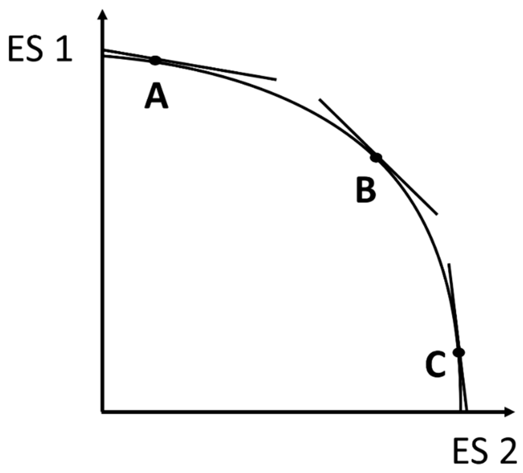
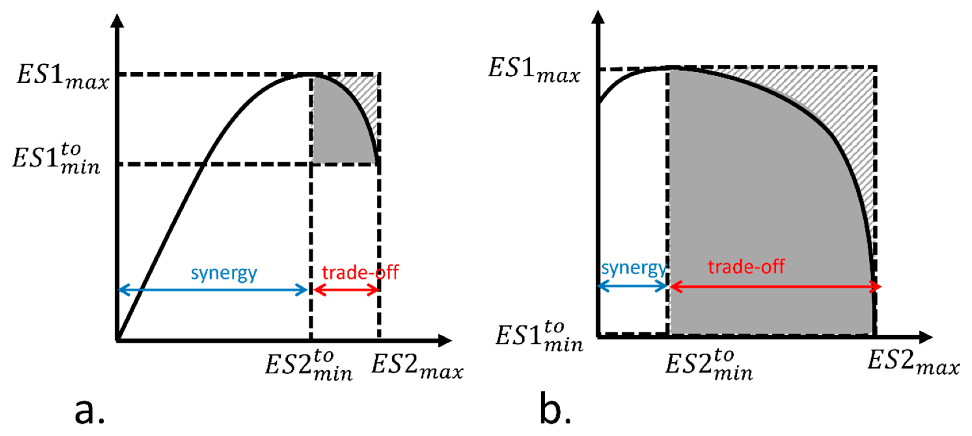
2. What Exactly Is Trade-Off in the PPF Context?

Surprisingly, explicit definitions of trade-off are rather rare in the ecosystem service and sustainability literature. Hopkins et al. [13] concur with this observation, noting that “at best, synergies are defined as causal positive relationships and trade-offs as causal negative relationship”. Cord et al. [14] also notice the rareness of explicit definitions of trade-offs, defining them as “an antagonistic situation that involves losing one quality of something in return for gaining another”. Deng et al. [15] reward us with the following definition: “In the ecosystem services context, the definition of trade-offs is mainly derived from the Millennium Ecosystem Assessment, which is defined as management choices that intentionally change the services provided by ecosystems”.
Considering specifically the studies that employ the PPF framework, it appears that most authors see no need for an explicit definition of trade-off, probably considering it an integral part of the PPF logic. It happens, in fact, that PPF curves are straightforwardly called “trade-off curves” [11]. However, both the commonplace understanding and the explicit definitions that the author was able to find in the literature are compatible with at least two interpretations in the PPF context—an ambiguity that can compromise any discussion of trade-off alleviation. We will now turn to the two interpretations.
The first interpretation is as the slope of the PPF curve at the given point (dES1/dES2). In economics, it is called the marginal rate of transformation (MRT). It corresponds to the amount of one ES that has to be given up for a marginal increase in the second ES. However, as MRT varies along the curve, so then must the trade-off severity (Figure 1). In addition, swapping the ESs changes the value of MRT inversely and the direction in which it increases. Consequently, according to this interpretation, the trade-off associated with a certain ES provision combination can be alleviated simply by changing the ES provision combination (i.e., moving from one to another point on the curve).
A second possible interpretation of trade-off is the PPF curve as a whole. This interpretation is cognitively more difficult as the curve represents a set of infinitely many trade-off situations with potentially different MRTs. Trade-off alleviation cannot, in this case, be conceived as moving from one point on the curve to another, rather it must imply a change in the whole curve. What curve represents a more severe trade-off and what a less severe is a question that calls for a whole-curve trade-off severity measure. The following sections will focus on the latter problem.

3. How to Measure Trade-Off Severity of a PPF?

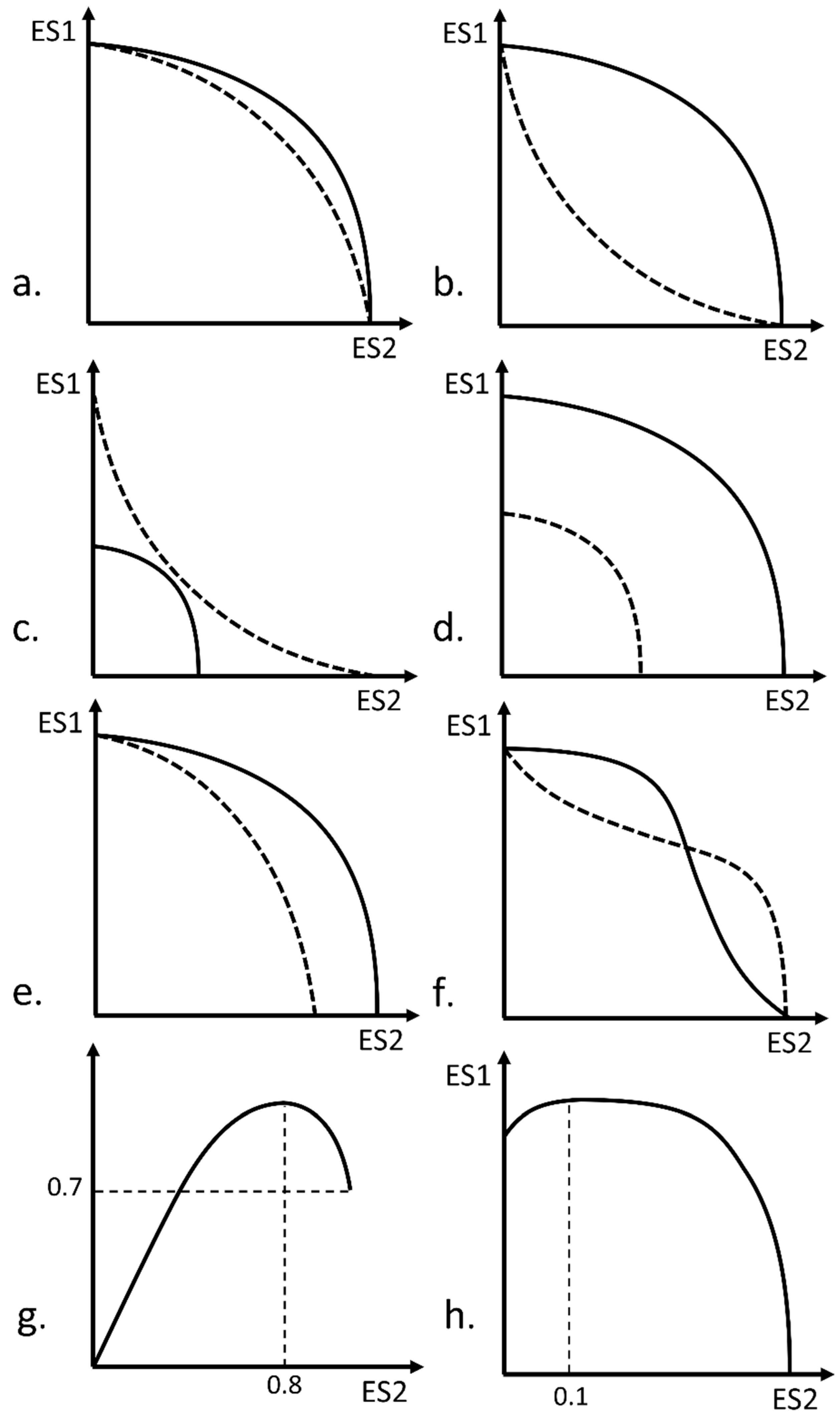
3.1. Requirements on a Generic Whole-Curve Trade-Off Severity Measure

An effective generic whole-curve trade-off severity measure should fulfill the following requirements.
  • The measure should be suited for comparing nested curves with coinciding or non-coinciding intercepts (the scales of the curve axes need not be normalized).
  • The measure should be able to handle crossing curves.
  • The measure should account for the relative range of trade-off.
  • The measure should not be limited to curves generated by any particular mathematical function.
Nested curves with overlapping intercepts (Figure 2a,b) constitute the most facile and intuitive case for comparison of trade-off severity. The more outward bent curve represents an ecosystem management framework subject to less severe trade-offs than the more inward bent curve. An example of comparisons made within such set of curves can be found in Bakx et al. [16] who analyze trade-offs between carbon storage and the financial value of forest harvests under different temporal and spatial constraints. Generally, the convex curve, such as the dashed-line curve in Figure 2b, is the archetype of strong trade-off and the concave curve, such as the curves in Figure 2a and the solid-line curve in Figure 2b, is that of weaker trade-off.
Nested curves with non-coinciding intercepts refer to the cases when the represented ecosystems or management frameworks differ in the maximum attainable levels of one or both ESs. Figure 2c shows a concave and a convex curve, Figure 2d a pair of parallel concave curves and Figure 2e a pair of non-parallel concave curves, all with non-coinciding intercepts. In this case the curvature is either different or the same, and the absolute amounts differ. A pair of parallel curves like in Figure 2d does not represent a change in the degree of conflict and thus cannot be considered trade-off alleviation, even though it constitutes a “win-win” (higher amounts of both services can be provided). A situation like in Figure 2e is discussed in Haight [5] referring to the effects of improvements in production technology on the decision maker’s chosen balance between production and non-provisioning ESs concluding that the improvements in production technology will further shift the balance towards production.
Crossing curves (Figure 2f) are challenging in that one of the curves is dominated by the other over a part of the range and vice versa. Thus, even with coinciding intercepts, it is difficult to judge which of them represents more severe trade-off. Crossing is more likely to occur when at least one of the curves is S-shaped. For example, in Mora et al. [17], S-shaped curves describe the plot level relationship between fodder and carbon stock and between fodder and species richness in a tropical dry forest region.
Finally, it is important to consider the possibility of a trade-off relationship being preceded by a positive (synergetic) relationship. This is a distinct feature of ES compared to technical production systems. For example, when bare land or a degraded ecosystem is the reference situation, increasing biomass stock will both deliver climate change mitigation benefits and allow for regular biomass harvest. Moreover, it will likely bring some biodiversity benefits. Matthies et al. [18] demonstrate how an initially synergetic relationship between climate mitigation benefits and biodiversity turns into trade-off in the later part of the outcome range. Thus, when assessing trade-off severity, the relationship between the outcome range with trade-off and the total outcome range need to be accounted for. For example, while in Figure 2g, a trade-off relationship ranges from 0.7 to 1 of ES1 and from 0.8 to 1 of ES2, in Figure 2h, it does so from 0 to 1 of ES1 and from 0.1 to 1 of ES2. The obvious intuition is that the trade-off relationship is more prominent in Figure 2h than in Figure 2f. It is likely that the failure to consider the full range of outcomes is one of the reasons for contradictory or inconclusive results of meta-analyses such as Lee and Lautenbach [19], concerning the nature (synergetic or trade-off) of the relationships within different ES pairs.

3.2. Current Approaches

The literature appears to agree with the intuitive idea that more outwards bent PPF curves constitute “weaker” [20], “mitigated” [21], “reduced” [17], or “alleviated” [22] trade-off. The author has been able to identify two common approaches to quantitative ES trade-off comparisons without clear origins and the formal trade-off severity measure proposed by Hegwood et al. [23].
A common way to quantify trade-off alleviation is to quantify the surplus, usually in relative terms, in one of the ESs somewhere along the range of the other (Figure 3). While this approach works for nested curves with coinciding intercepts, crossed curves cannot be meaningfully compared in this way. Furthermore, it may lead to a wrong conclusion concerning trade-off alleviation in case of parallel curves like in Figure 2d.
In some studies, the trade-off relationship between the features in question is defined by a specific function containing a parameter controlling the curve shape. The parameter is then used to communicate trade-off severity. For example, Egas et al. [20] use the following model to describe the relationship between the levels of a species’ specialization on two types of habitats.
( e i 1 ) 1 s + ( e i 2 ) 1 s = 1
where e i 1 and e i 2 are foraging efficiencies in habitat 1 and 2, respectively, and s is a curve shape parameter interpreted as trade-off strength. The relationship is convex with s < 1 (“strong trade-off”) and concave with s > 1 (“weak trade-off”); with s = 1, the relationship is linear. The obvious shortcoming of this approach is that the measure only exists within a particular model.
Hegwood et al. [23] present an original trade-off severity measure defined as the largest fraction X(n) of the maximum possible value of each of the n objectives that can be achieved simultaneously (Figure 4). For example, if X(2) = 0.8, the highest simultaneous attainment of two objective is 80% of their maxima. This measure is somewhat like the first of those presented in this chapter in that it focuses on the position of a single point on the curve rather than capturing the whole “outwards-bendedness” of the curve.

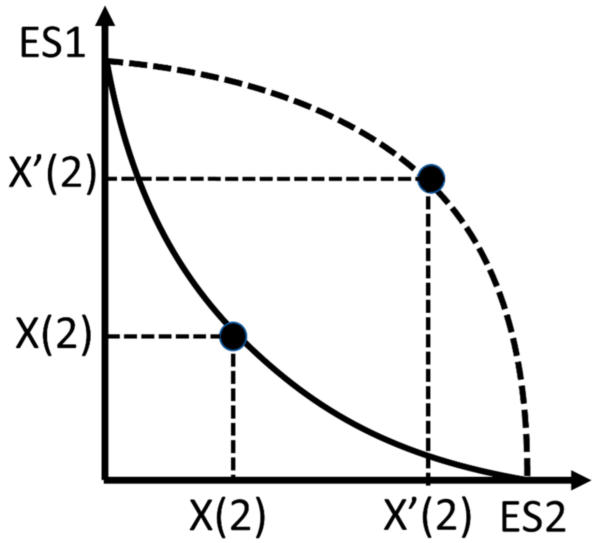
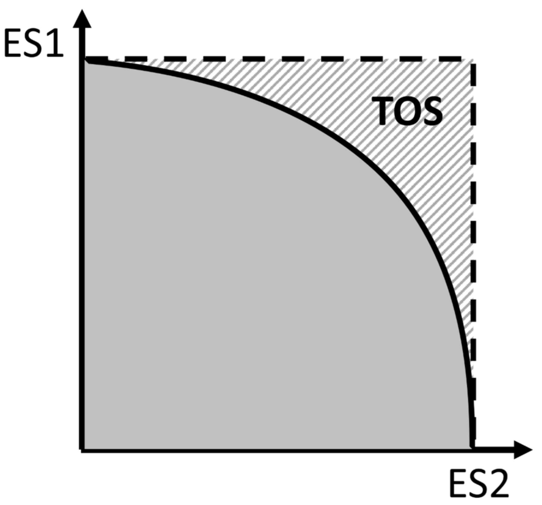
4. A Generic Whole-Curve Trade-Off Severity Measure
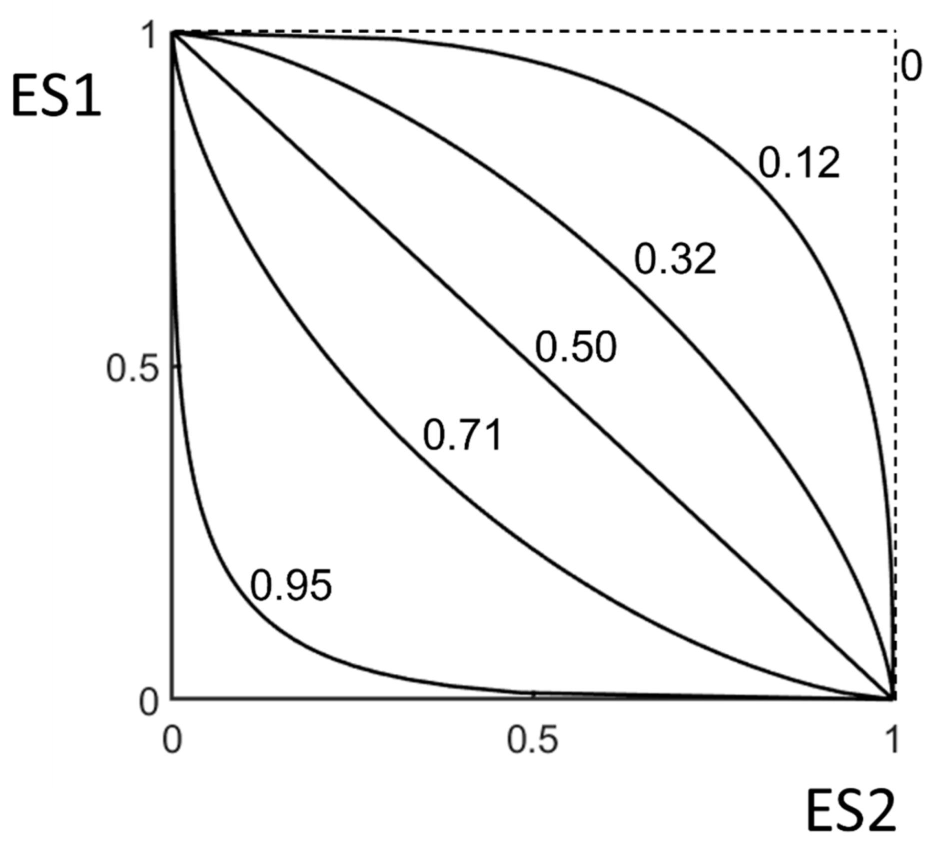
The author proposes to measure trade-off severity as the ratio between the area above the PPF curve (within the smallest rectangular encompassing the curve) and the total area of the smallest rectangular encompassing the curve (Figure 5). The area above the curve is calculated as the difference between the area of the rectangular and the area under the curve obtained by integration. For mathematical expression, let a PPF curve be defined by the function ES1 = f(ES2), ES1max and ES2max denote the extremes of ES1 and ES2, respectively. The trade-off severity TOS is then defined by Equation (2).
T O S = E S 1 m a x × E S 2 m a x f E S 2 d E S 2 E S 1 m a x × E S 2 m a x
In the case of normalized scales (i.e., ranging between 0 and 1), the product of the ESs maxima is equal to one, and the expression takes the form of Equation (3).
T O S = 1 f E S 2 d E S 2
Thus, when the shape of PPF is rectangular, TOS = 0, and there exists no trade-off between the ESs: ES1 stays at its maximum level regardless of the level of ES2 and vice-versa. When TOS = 1, the trade-off is absolute: as soon as ES1 > 0, ES2 is zero, and vice-versa. All the intermediate situations fall between TOS zero and one.
The multi-dimensional case, with n E S x where x = 1 … n and E S 1 = f E S 2 , , E S n , is handled according to Equations (4) and (5), which are generalizations of Equations (1) and (2), correspondingly. Here E S x m a x denotes the extreme of E S x .
T O S = x = 1 n E S x m a x f E S 2 , , E S n d E S 2 , , d E S n x = 1 n E S x m a x
T O S = 1 f E S 2 , , E S n d E S 2 , , d E S n
To account for the relative range of trade-off, Equation (1) is modified by multiplication with the ratio between the product of the trade-off ranges of each ES and the product of their total ranges (Equation (6) and Figure 6). Since consideration of the relative trade-off range in calculating TOS can result in widely different values than TOS calculated without such consideration, a new notation—TOSra—is introduced for the range-adjusted trade-off severity measure. Equation (6) defines TOSra for the two-dimensional case with ES1 and ES2.
T O S r a = ( E S 1 m a x E S 1 m i n t o ) × ( E S 2 m a x E S 2 m i n t o ) E S 1 m a x × E S 2 m a x × ( E S 1 m a x E S 1 m i n t o ) × ( E S 2 m a x E S 2 m i n t o ) E S 2 m i n t o E S 2 m a x E S 2 d E S 2 ( E S 1 m a x E S 1 m i n t o ) × ( E S 2 m a x E S 2 m i n t o ) = ( E S 1 m a x E S 1 m i n t o ) × ( E S 2 m a x E S 2 m i n t o ) E S 2 m i n t o E S 2 m a x E S 2 d E S 2 E S 1 m a x × E S 2 m a x
E S 1 m a x and E S 1 m i n t o denote the maximum of the range and the lower limit of the trade-off range for ES1, with corresponding notations for ES2. This is different from the initial mode of calculation in Equations (2)–(5) where the trade-off relationship was assumed to take place over the entire range (0; max) of the ES outcomes. Thus, Equations (2) and (3) are special cases of Equation (6).
Equation (7) generalizes Equation (6) for multiple dimensions, with ESx where x = 1 … n is modified. All the previous equations are special cases of Equation (7).
T O S r a = x = 1 n ( E S x m a x E S x t o   m i n ) t o   m i n m a x f E S 2 ,   , E S n   d E S 2 , , d E S n x = 1 n E S x m a x
Noteworthy, the trade-off severity measure presented here can also be used to mathematically prove the statement that Hegwood et al. [10] prove using their severity measure: that, with the number of ESs approaching infinity, the trade-off severity approaches its maximum regardless of the curvature of the trade-off surface. With E S x m a x = 1 and E S x t o   m i n = 0, the calculation of volume under the PPF surface by multiple integration will involve raising of some number between zero and one (exclusively) to the power of n, which, with n approaching infinity, will result in zero. With other equation terms being equal to 1, TOS or TOSra will also be equal to 1. With E S x t o   m i n > 0 and n approaching infinity, TOSra does not exist as it implies division by zero.

5. Example

Figure 7 presents TOS for a set of curves based on Equation (1) from Egas et al. [20] with s = 4, 1.5, 1, 0.6667, 0.25. Note that the innermost and the outermost curves, which appear to be symmetric according to the values of s (4 and 0.25), are not so according to TOS (0.95 and 0.12).

6. Conclusions

This paper discusses the concepts of trade-off, trade-off severity and trade-off alleviation in the PPF context. It is suggested that the whole-curve interpretation of trade-off is more robust than the local curve-slope interpretation. The scrutiny of the current ways of measuring and communicating trade-off severity leads to the conclusion that they are unable to support trade-off comparisons except in narrowly defined cases. Furthermore, they, except the measure developed by Hegwood et al. [23], fail to draw distinction between trade-off alleviation proper and situations that imply a simultaneous increase in the provision of two or more ESs (win–win) with unchanged trade-off severity. As a remedy, a generic whole-curve quantitative measure of trade-off severity (TOS) is proposed. TOS can be applied to curves of any shapes, crossing and non-crossing, as well as surfaces in multidimensional spaces, in order to support comparisons of ES trade-offs under different ecosystem management frameworks or, indeed, applied in trade-off analyses in any other field. In addition, a special variant of the measure (TOSra) is proposed that accounts for the often-dual nature of the relationship between ES: an initial synergy and the ensuing trade-off.

Funding

The work has been funded by Formas, a Swedish research council for sustainable development (Grant Nr FR-2021/0004).

Acknowledgments

The author thanks Cecilia Akselsson, Henrik Smith, and other members of the ForestPath project for stimulating discussions.

Conflicts of Interest

The author declares no conflict of interest.

References

  1. Bakx, T.R.; Trubins, R.; Eggers, J.; Akselsson, C. The effect of spatial and temporal planning scale on the trade-off between the financial value and carbon storage in production forests. Land Use Policy 2023, 127, 106583. [Google Scholar] [CrossRef]
  2. Bekele, E.G.; Lant, C.L.; Soman, S.; Misgna, G. The evolution and empirical estimation of ecological-economic production possibilities frontiers. Ecol. Econ. 2013, 90, 1–9. [Google Scholar] [CrossRef]
  3. Björklund, J.; Limburg, K.E.; Rydberg, T. Impact of production intensity on the ability of the agricultural landscape to generate ecosystem services: An example from Sweden. Ecol. Econ. 1999, 29, 269–291. [Google Scholar] [CrossRef]
  4. Cavender-Bares, J.; Polasky, S.; King, E.; Balvanera, P. A sustainability framework for assessing trade-offs in ecosystem services. Ecol. Soc. 2015, 20, 56. [Google Scholar] [CrossRef]
  5. Cord, A.F.; Bartkowski, B.; Beckmann, M.; Dittrich, A.; Hermans-Neumann, K.; Kaim, A.; Lienhoop, N.; Locher-Krause, K.; Priess, J.; Schröter-Schlaack, C.; et al. Towards systematic analyses of ecosystem service trade-offs and synergies: Main concepts, methods and the road ahead. Ecosyst. Serv. 2017, 28, 264–272. [Google Scholar] [CrossRef]
  6. DeFries, R.S.; Foley, J.A.; Asner, G.P. Land-use choices: Balancing human needs and ecosystem function. Front. Ecol. Environ. 2004, 2, 249–257. [Google Scholar] [CrossRef]
  7. Deng, X.; Li, Z.; Gibson, J. A review on trade-off analysis of ecosystem services for sustainable land-use management. J. Geogr. Sci. 2016, 26, 953–968. [Google Scholar] [CrossRef]
  8. Egas, M.; Dieckmann, U.; Sabelis, M.W. Evolution Restricts the Coexistence of Specialists and Generalists: The Role of Trade-off Structure. Am. Nat. 2004, 163, 518–531. [Google Scholar] [CrossRef]
  9. Haight, A.D. Diagram for a small planet: The Production and Ecosystem Possibilities Curve. Ecol. Econ. 2007, 64, 224–232. [Google Scholar] [CrossRef]
  10. Hegwood, M.; Langendorf, R.E.; Burgess, M.G. Why win–wins are rare in complex environmental management. Nat. Sustain. 2022, 5, 674–680. [Google Scholar] [CrossRef]
  11. Hopkins, S.R.; Sokolow, S.H.; Buck, J.C.; De Leo, G.A.; Jones, I.J.; Kwong, L.H.; LeBoa, C.; Lund, A.J.; MacDonald, A.J.; Nova, N.; et al. How to identify win–win interventions that benefit human health and conservation. Nat. Sustain. 2021, 4, 298–304. [Google Scholar] [CrossRef]
  12. Juutinen, A.; Saarimaa, M.; Ojanen, P.; Sarkkola, S.; Haara, A.; Karhu, J.; Nieminen, M.; Minkkinen, K.; Penttilä, T.; Laatikainen, M.; et al. Trade-offs between economic returns, biodiversity, and ecosystem services in the selection of energy peat production sites. Ecosyst. Serv. 2019, 40, 101027. [Google Scholar] [CrossRef]
  13. King, E.; Cavender-Bares, J.; Balvanera, P.; Mwampamba, T.H.; Polasky, S. Trade-offs in ecosystem services and varying stakeholder preferences: Evaluating conflicts, obstacles, and opportunities. Ecol. Soc. 2015, 20, 15. [Google Scholar] [CrossRef]
  14. Lee, H.; Lautenbach, S. A quantitative review of relationships between ecosystem services. Ecol. Indic. 2016, 66, 340–351. [Google Scholar] [CrossRef]
  15. Lester, S.E.; Costello, C.; Halpern, B.S.; Gaines, S.D.; White, C.; Barth, J.A. Evaluating tradeoffs among ecosystem services to inform marine spatial planning. Mar. Policy 2013, 38, 80–89. [Google Scholar] [CrossRef]
  16. Matthies, B.D.; Kalliokoski, T.; Eyvindson, K.; Honkela, N.; Hukkinen, J.I.; Kuusinen, N.J.; Räisänen, P.; Valsta, L.T. Nudging service providers and assessing service trade-offs to reduce the social inefficiencies of payments for ecosystem services schemes. Environ. Sci. Policy 2016, 55, 228–237. [Google Scholar] [CrossRef]
  17. Mora, F.; Balvanera, P.; García-Frapolli, E.; Castillo, A.; Trilleras, J.M.; Cohen-Salgado, D.; Salmerón, O. Trade-offs between ecosystem services and alternative pathways toward sustainability in a tropical dry forest region. Ecol. Soc. 2016, 21, 13. [Google Scholar] [CrossRef]
  18. Nelson, E.; Polasky, S.; Lewis, D.J.; Plantinga, A.J.; Lonsdorf, E.; White, D.; Bael, D.; Lawler, J.J. Efficiency of incentives to jointly increase carbon sequestration and species conservation on a landscape. Proc. Natl. Acad. Sci. USA 2008, 105, 9471–9476. [Google Scholar] [CrossRef]
  19. Phalan, B.; Onial, M.; Balmford, A.; Green, R.E. Reconciling Food Production and Biodiversity Conservation: Land Sharing and Land Sparing Compared. Science 2011, 333, 1289–1291. [Google Scholar] [CrossRef]
  20. Pohjanmies, T.; Eyvindson, K.; Triviño, M.; Mönkkönen, M. More is more? Forest management allocation at different spatial scales to mitigate conflicts between ecosystem services. Landsc. Ecol. 2017, 32, 2337–2349. [Google Scholar] [CrossRef]
  21. Rohweder, M.R.; McKetta, C.W.; Riggs, R.A. Economic and Biological Compatibility of Timber and Wildlife Production: An Illustrative Use of Production Possibilities Frontier. Wildl. Soc. Bull. 2000, 28, 435–447. [Google Scholar]
  22. Rolo, V.; Roces-Diaz, J.V.; Torralba, M.; Kay, S.; Fagerholm, N.; Aviron, S.; Burgess, P.; Crous-Duran, J.; Ferreiro-Dominguez, N.; Graves, A.; et al. Mixtures of forest and agroforestry alleviate trade-offs between ecosystem services in European rural landscapes. Ecosyst. Serv. 2021, 50, 101318. [Google Scholar] [CrossRef]
  23. Smith, F.P.; Gorddard, R.; House, A.P.; McIntyre, S.; Prober, S.M. Biodiversity and agriculture: Production frontiers as a framework for exploring trade-offs and evaluating policy. Environ. Sci. Policy 2012, 23, 85–94. [Google Scholar] [CrossRef]
Figure 1. Directionality and variability of MRT along a PPF curve. The value of MRT—the slope of the curve—is different at points A, B and C. If expressed in terms of the change in ES1 for a change in ES2 (dES1/dES2), the MRT is increasing from A to C. In the inverse case (dES2/dES1), it is increasing from C to A.
Sustainability 15 16763 g001
Figure 2. Examples of PPF curves. (a) Two concave curves with shared intercepts but with different outward bents. (b) A concave (solid line) and a convex (dashed line) curves with shared intercepts. (c) A concave (solid line) and a convex (dashed line) curves with different intercepts. (d) Two parallel concave curves. (e) Two concave curves meeting at one of two intercepts (f) Two crossing s-shaped curves. (g,h) Two curves with different relative ranges of positive (synergetic) and trade-off relationships.
Sustainability 15 16763 g002
Figure 3. Comparing two PPF curves by measuring the increase in ES1 at an arbitrary point of ES2 range. P(ES1) is the provision of ES1 according to the dashed curve and P*(ES1) is the provision level of ES1 according to the solid curve, both at the provision P(ES2) of ES2.
Sustainability 15 16763 g003
Figure 4. The trade-off severity measure of Hegwood et al. [10]. With n = 2 dimensions, X(2) and X′(2) is the maximum relative simultaneous provision of ES1 and ES2 for, respectively, the solid and the dashed curves. X’(2) > X(2), thus, the trade-off severity of the former curve is less.
Sustainability 15 16763 g004
Figure 5. The trade-off severity measure TOS. The area difference between the rectangular shape encompassing the PPF curve and the area under the PPF curve (divided by the area of the rectangular) quantifies the trade-off severity of the given PPF.
Sustainability 15 16763 g005
Figure 6. Examples of different relative ranges of synergetic and trade-off relationships between ES. (a) The synergetic relationship range is large compared to the trade-off range. (b) The synergetic relationship range is small compared to the trade-off range. The rectangular area encompassing the entire curve (0; ES1max) and (0; ES2max) is used to weigh TOS calculated within the range of the trade-off relationship (shaded and patterned) ( E S 1 m i n t o ; ES1max) and ( E S 2 m i n t o ; ES2max).
Sustainability 15 16763 g006
Figure 7. A set of PPF curves with TOS values.
Sustainability 15 16763 g007
Disclaimer/Publisher’s Note: The statements, opinions and data contained in all publications are solely those of the individual author(s) and contributor(s) and not of MDPI and/or the editor(s). MDPI and/or the editor(s) disclaim responsibility for any injury to people or property resulting from any ideas, methods, instructions or products referred to in the content.

