Article

Anthropogenic Drivers of Hourly Air Pollutant Change in an Urban Environment during 2019–2021—A Case Study in Wuhan

1
School of Remote Sensing and Information Engineering, Wuhan University, Wuhan 430079, China
2
Hubei Eco-Environmental Monitoring Centre, Wuhan 430079, China
3
Department of Land Surveying and Geo-Informatics, The Hong Kong Polytechnic University, Hong Kong 999077, China
*
Author to whom correspondence should be addressed.
Sustainability 2023, 15(24), 16694; https://doi.org/10.3390/su152416694
Submission received: 1 November 2023 / Revised: 1 December 2023 / Accepted: 4 December 2023 / Published: 9 December 2023

Abstract

:
Wuhan experienced a noticeable enhancement in air quality from January to April 2020 due to the epidemic lockdown. The improvement was a combined result of anthropogenic emission reduction and meteorological variability. Environmental policymakers are often concerned about the impact of industrial production and human activities on improvements in environmental sustainability. This study split and quantified the impact of anthropogenic emissions on the pollution level changes of six major air pollutants (CO, SO2, NO2, O3, PM10, and PM2.5) for the first half year of 2019 to 2021 in Wuhan with an improved meteorological normalization algorithm. The results show sharp decreases in anthropogenic pollutant loads during 2020, except for O3, with the ranking of NO2 > PM10 > SO2 > CO > PM2.5. The decrease in NO2 emissions caused by humans was more than 50% compared to 2019. The low NO2 led to a decrease in O3 consumption, resulting in high O3 concentrations from February to April 2020 during the city lockdown. Moreover, except O3, the impact of anthropogenic and weather influences on air pollution exhibited opposing effects; that is, meteorology tended to aggravate pollution, while human intervention was conducive to improving air quality, and human factors played the dominant role. Of all six pollutants, O3 is the one that is relatively least subject to anthropogenic emissions. Although concentrations of SO2, NO2, PM10, and PM2.5 rebounded in 2021, none of them were able to return to their pre-lockdown levels, suggesting the epidemic’s continuous inhibition of people’s activities. Compared with 2019 and 2021, the atmospheric oxidation capacity and secondary aerosol formation showed an overall decreasing trend during 2020. This study provides a reference for assessing the effectiveness of anthropogenic emission reduction policies.

1. Introduction

With the fast progress of industry and urbanization, substantial quantities of human-made pollutants, such as CO, SO2, NO2, O3, and PM, have led to the deterioration of air quality in China, causing great harm to public health and, hence, arousing wide concern for sustainable development [1]. Wuhan is one of the most populous cities in central China, where air quality is affected by a combination of natural (e.g., terrain and meteorology) and man-made factors (e.g., industrial and vehicle emissions) [2,3]. When examining trends in different pollutant species, it could prove difficult to distinguish whether a change in pollutant concentration is due to weather or a modification in emission source. The observed alterations in pollutants might be influenced by meteorological fluctuations rather than emission-induced disturbances, which can result in an inaccurate evaluation of the efficacy of emission reduction policy for urban sustainability if meteorology is not regulated or considered [4,5].
From 2019 to 2021, Wuhan experienced a pre-epidemic, an epidemic lockdown, and a post-epidemic recovery period. This uncommon episode became an extreme intervention incident, presenting a valuable opportunity to gain a deeper understanding of the anthropogenic effects governing pollutant trends and urban environmental change in Wuhan [6,7,8,9]. Lu et al. [10] employed WRF-CMAQ to model the impact of both meteorological factors and human activities on the levels of PM2.5 in various cities throughout China from January to March 2020. They highlighted that a combination of better weather conditions and a significant decrease in pollutant emissions contributed to the reduction of PM2.5 levels in Wuhan, which was higher than the national average. However, Zhou et al. [11] argued that the decline in simulated PM2.5 levels in Wuhan during the epidemic was attributed to the decrease in anthropogenic emissions, whereas meteorology aggravated PM2.5 pollution. The contradictory simulations can be attributed to the high level of uncertainty in the meteorological initial fields and emission inventories used in the models. To validate these simulations, it is also necessary to verify them by observations. In addition to model-based research, Mateusz et al. [12] explored the use of big data-driven machine learning techniques for analyzing the pandemic’s spatiotemporal patterns of air pollution in Poland and revealed a distinct clustering pattern of PM10.
Meteorological normalization provides a new perspective to quantifying anthropogenic effects on sustainable management of air quality based on observations rather than models and is used to explain the cause of regional haze [5,13]. In general, meteorological normalization employs a machine learning algorithm (MLA) to predict pollutant concentrations under a normalized meteorological condition, and their changes are regarded as anthropogenic contributions. Qu et al. [14] obtained a meteorologically normalized distribution of PM2.5 based on an MLA of a boosted regression tree. Their results show that the adoption of policies aimed at reducing emissions between 2014 and 2019 led to a 60% reduction in the yearly average concentration of anthropogenic PM2.5 in the Beijing–Tianjin–Hebei area [15]. Huang et al. [8] investigated the variations in the chemical constituents of PM2.5 on an hourly basis in Wuhan during the first month of lockdown and compared the results to the same timeframe in 2019, using a meteorological normalization algorithm proposed by Grange and Carslaw [5] and positive definite factorization theories. Their findings show that the decrease in anthropogenic emissions accounted for 92% of the overall reduction in PM2.5 levels during the initial month of the lockdown, with meteorology contributing the remaining 8%. They also discovered that the considerable rise in atmospheric oxidation rates, which was responsible for the drop in primary aerosol concentrations, was also responsible for an increase in secondary aerosol formation. This partly explains why regional haze pollution events still occurred during the lockdown period [9].
The aforementioned studies have made significant strides in evaluating the effects of anthropogenic emission reductions on the enhancement of air quality during the lockdown. The epidemic has changed the behavior patterns of the public [16,17]. Therefore, policymakers are concerned about the impact of anthropogenic activity in the post-lockdown period, an aspect that has not been adequately addressed in current research. In addition, most studies focus on PM2.5, while other pollutants, such as O3 and NO2, have not been sufficiently analyzed. To this end, based on long-term observation, the present study examines the contributions of anthropogenic and meteorological factors to the levels of six major pollutants in Wuhan before, during, and after the lockdown period (from January to May 2019, 2020, and 2021) by applying the meteorological normalization with an MLA of a parameter self-optimized boosted regression tree. Moreover, the atmospheric oxidation capacity and secondary aerosol generation are also investigated to reveal the association between primary emissions and secondary pollution. This investigation could serve as a point of reference for governmental organizations to conduct a more comprehensive evaluation of the efficacy of pollution control policies.

2. Materials and Methods

2.1. Data

Wuhan, situated between 113°41′–115°05′ E and 29°58′–31°22′ N, is the largest city in Central China. As of 2019, the city boasts a permanent population of 11.212 million. The landforms in Wuhan are characterized by platforms and plains with low elevations and gentle slopes (Figure 1). The Yangtze River, the third-largest river in the world, flows through the city. Wuhan has the largest freshwater area in China, accounting for approximately a quarter of its total area. The city has a humid subtropical monsoon climate with ample sunshine. The annual average temperature ranges from approximately 15.8 °C to 17.5 °C, and the annual rainfall exceeds 1150 mm. The annual average wind speed in Wuhan is about 2.7 m/s. During summer, southerly and southeasterly winds prevail, while northerly and northeasterly winds dominate in winter [1].
The data utilized in this study was gathered from an observatory situated on the rooftop of the Hubei Ecological and Environmental Monitoring Center in Wuhan, Hubei Province of China, positioned approximately 16 m above the ground level (114.37° E, 30.53° N). The air quality here is mainly affected by emissions from industry, traffic, construction, etc. Various devices are used for sampling different data. Specifically, CO concentrations were obtained by a correlated infrared absorption analyzer (TAPI 300E, Teledyne API, San Diego, CA, USA). A Casella ML9841B chemiluminescent trace NO-NO2-NOx analyzer (Casella Measurement Ltd., Bedford, UK) was utilized to measure NO2 levels. O3 and SO2 levels were measured using a TEI 49i UV photometric ozone analyzer (Thermo Fisher Scientific, Franklin, MA, USA) and a Casella ML9850B pulsed UV fluorescence SO2 analyzer (Casella Measurement Ltd., Bedford, UK), respectively. An oscillating balance analyzer with two separate inlets (model TH-2000Z, Wuhan Tianhong Environmental Protection Industry Co., Ltd., Wuhan, China) was used to measure PM10 and PM2.5 levels. The SO42− and NO3 ions used in the secondary aerosol generation analysis were obtained from a MARGA (Monitor for AeRosols and GAses) online ion analyzer (model: ADI 2080, Metrohm, Auckland, New Zealand) developed by the Energy Research Center in the Netherlands. In addition to the pollutants, various meteorological parameters, including wind speed (WS, m/s), wind direction (WD, °), temperature (T, °C), relative humidity (RH, %), and atmospheric pressure (P, hPa), were concurrently obtained through on-site measurements. The collection equipment consisted of temperature and humidity sensors, rain gauges, wind speed sensors, wind direction sensors, and other devices. The Hubei Ecological Environment Monitoring Center Station was responsible for data collection and preliminary quality control. Only data that satisfied the quality standards stipulated by the local environmental agency were utilized in this study.
A total of 10,895 samples from 1 January to 31 May for three consecutive years (2019, 2020, and 2021) were collected finally. Each sample encompassed 13 observed parameters, with a temporal resolution of 1 h. These parameters included mass concentrations of six pollutants (CO, SO2, NO2, O3, PM2.5, and PM10), five meteorological parameters (WS, WD, T, RH, and P), as well as two secondary inorganic water-soluble ions (SO42− and NO3, μg/m3). We used three times standard deviation as a constraint to filter abnormally large data. Then, for the original missing or filtered missing records, the average strategy with a 3-day sliding window was applied, resulting in a record missing rate of less than 5%.

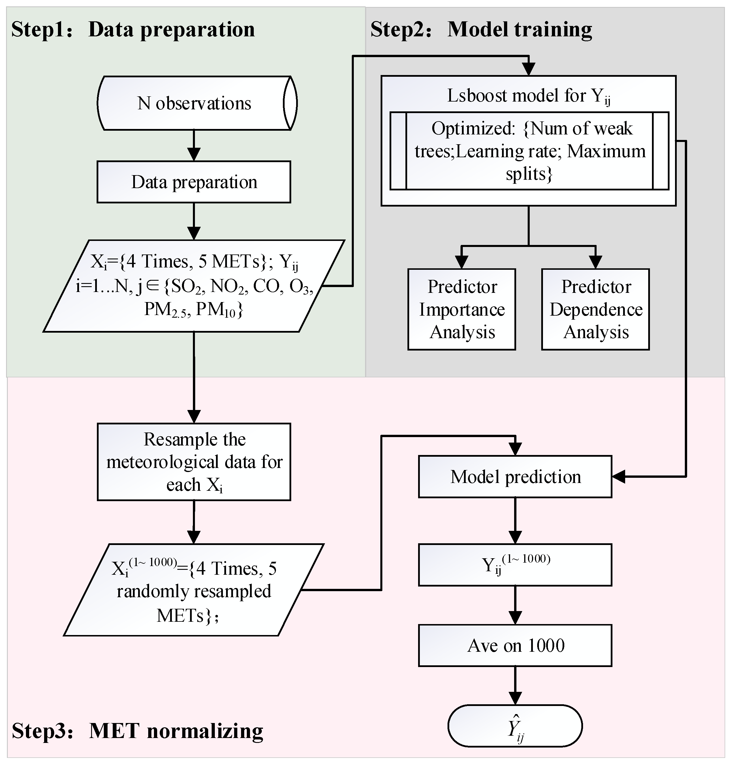
2.2. Meteorological Normalization by a Self-Optimized Boosted Regression Tree Model

Quantifying the anthropogenic effect on air pollution has been a long-term challenge in terms of the covarying meteorological influence. Here, we apply a meteorological normalization technique to separate the man-made influence from the meteorological effect [5,13,18]. By utilizing temporal and meteorological variables as inputs, the MLA regression model is constructed to respectively forecast the concentrations of six pollutants. The meteorologically normalized pollution concentrations are obtained by averaging the predicted concentrations for each observation with resampled meteorological variable values.
The random forest model is frequently utilized for MLA regression, necessitating the manual predefinition of model parameters, such as the learning rate and maximum tree split. To ensure the accuracy and calculation efficiency of the regression model over a large volume of input samples, this research adopts a parameter self-optimized boosted regression tree named as the boosted least squares integrated regression tree model (LSBoost). The fundamental idea of LSBoost is to gradually enhance the predictive power of the model by iteratively adding weak learners to form a strong learner. Boosting begins with a constant prediction and grows a sequence of trees. With each subsequent step, a new tree is progressively added to the model, resulting in an increasingly accurate prediction [19]. The whole process is realized by the following 3 steps, which have also been summarized in Figure 2:
Firstly, data preparation for a regression model is performed on all observation samples. We obtain input vectors of Xi (I = 1, …, N, N = 10895) containing 4 temporal (Times, including Julian day, day of the year (DOY), day of the month (DOM), and weekday) and 5 meteorological variables (METs, including WS, WD, T, RH, and P), and the respective 6 output variables of Yij (j = 1, 2, 3, 4, 5, 6, indicating concentrations of 6 key pollutants).
Secondly, regression models are trained with 4 Times and 5 METs variables to predict 6 pollutant concentrations, respectively. In our algorithm, the regression tree in the weak learners uses the agent node to compensate for the regression bias caused by some missing data. The model found optimal hyperparameters (Number of weak trees, Learning rate, and Maximum splits) automatically using Bayesian optimization. The trained LSBoost models are also employed to assess the importance of predictors and partial dependence for 6 pollutants. Table 1 illustrates the self-learning model parameters and performance metrics, with a training R2 value exceeding 0.98 when the training and test sets are identical.
Thirdly, the anthropogenic contribution is quantified through meteorological normalization. The renewed meteorological quintuplet is randomly selected from all meteorological observations, but the 4 Times parameters of each input vector are kept unchanged. The above well-trained models are used to predict 6 pollutant concentrations, respectively, with the renewed input vector. The above process is repeated 1000 times. The average of the 1000 predictions is termed the normalized pollution level ( Y ^ i j ), as it represents the pollutant under a statistically average meteorological condition [16].  Y ^ i j  can be used to denote the anthropogenic effect [8,20]. The difference between observations and normalized concentrations can be considered as the meteorology-induced contribution.

2.3. Atmospheric Oxidation and Aerosol Secondary Generation Capability

Studies [8] have reported an increase in the production of secondary aerosols, specifically sulfate, and nitrate, during the lockdown period. To analyze atmospheric oxidation and secondary aerosol production before and after the city lockdown, the total concentration of O3 and NO2 (referred to as Ox) was utilized to characterize atmospheric oxidation capacity [8]. Moreover, as CO primarily arises from anthropogenic primary emissions, the PM2.5/CO ratio can serve as an indicator of secondary aerosol formation [9]. Additionally, the conversion rate of gaseous NO2 and SO2 to solid NO3 and SO42−, the primary sources of secondary inorganic aerosols, can be quantified by the nitrogen oxidation rate (NOR) and sulfur oxidation rate (SOR), respectively. These rates are defined as follows [21,22,23]:
S O R = S O 4 2 S O 4 2 + S O 2 ,
N O R = N O 3 N O 3 + N O 2 ,
where  S O 4 2 S O 2 N O 3 N O 2  are the molar concentrations of SO42−, NO3, SO2, and NO2. According to previous studies [24], the SOR(NOR) in primary pollutants is typically below 0.10. Higher values suggest more oxidation of precursor gases and significant production of nitrates and sulfates.

3. Results and Discussion

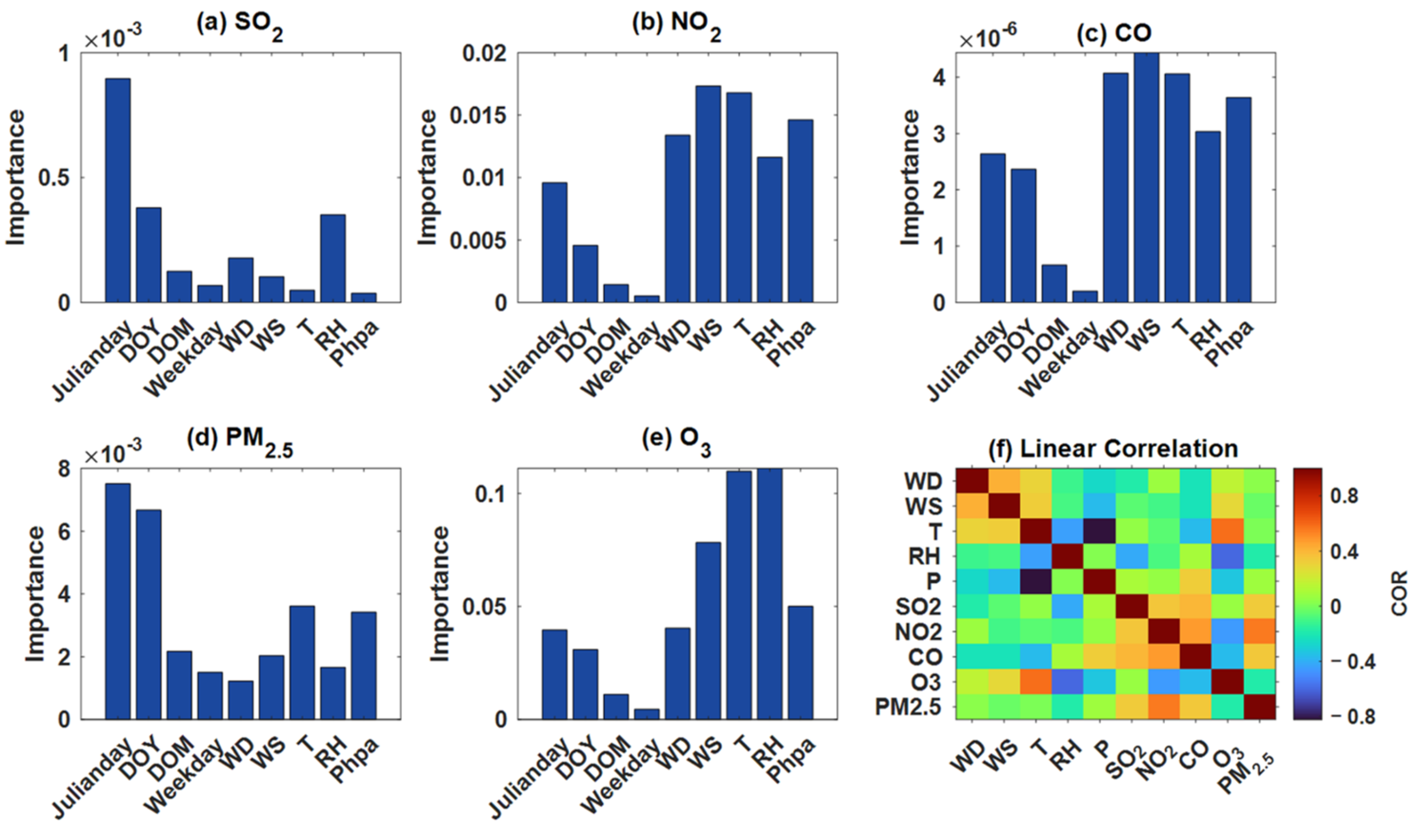
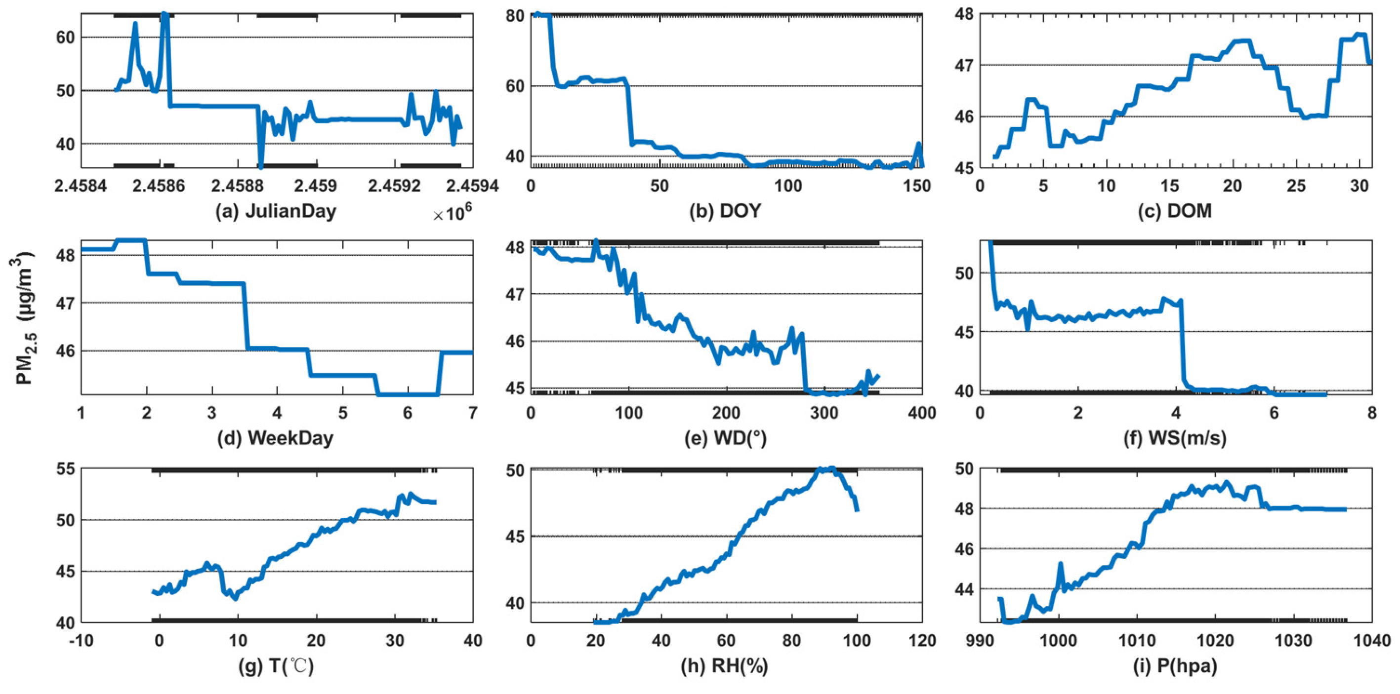
3.1. Meteorology Importance on Pollutants Based on LSBoost

The LSBoost model is employed to assess the relative importance and the potential factors associated with the six key pollutants. Larger importance indicates that the predictor contributes more significantly to the response variable. The importance of meteorology parameters (Julian day, DOY, DOM, weekday, WD, WS, T, RH, Phpa) for the learning of pollutant variables and their linear correlation are shown in Figure 3.
As seen in Figure 3a–e, the most important meteorological factors for NO2, CO, and O3 are WD, WS, T, and RH. The prevailing winds dominate the dispersal and transport of gaseous pollutants. Higher wind speeds can help dilute pollutants and displace them over longer distances, leading to lower pollutant concentrations. Atmospheric chemical reactions, including photochemical reactions and aqueous phase reactions stimulated by moisture, are important factors influencing the formation of particulate matter [25]. Optimal conditions for photochemical synthesis involve high temperature and low humidity, which can lead to increased rates of synthesis and higher concentrations of NO2 and CO [26,27]. High concentrations of O3 frequently occur in hot, dry, inactive environments, which are beneficial to O3 generation and persistence [27]. PM2.5 and SO2 are less influenced by meteorological conditions when compared to NO2, CO, and O3. Their changes tend to exhibit a stronger temporal and seasonal periodicity as they are more influenced by time variables [20]. It can also be seen from Figure 3f that SO2 has a strong negative correlation with RH. NO2 and PM2.5 show a weak negative correlation with meteorological factors. CO has a negative correlation with wind speed and temperature and a positive correlation with surface pressure. And O3 has a more significant positive correlation with temperature and a negative correlation with RH, which implies the promotion of O3 secondary production by active photochemical reactions under such meteorology environments.
Air pollutants are influenced by both time and meteorological parameters, as shown by the partial dependence of the predicted six target pollutants on these factors in Figure 4. Figure 4a displays the distribution of PM2.5 based on Julian day. The average concentration of PM2.5 exhibits a noticeable decrease in 2020, followed by a slight increase in 2021, relative to 2019, during the first half-year intervals from January to May. PM2.5 levels in Wuhan are higher during the winter months (DOY < 60 in Figure 4b), a phenomenon that can be attributed to increased pollutant emissions resulting from coal combustion [28]. And PM2.5 has relatively high concentrations in the middle of the month and on weekdays, which aligns with the results reported by Sun et al. [29]. Furthermore, the concentration of PM2.5 exhibits a dependence on wind direction and speed. Pollutants are easily transported from the north to Wuhan, driven by prevailing winds with WD < 100°. The static weather characterized by low wind speed (WS < 4 m/s) would further exacerbate pollution by promoting the local accumulation of pollutants. In addition, PM2.5 increases approximately linearly with increasing temperature as a result of strong photochemical reactions that convert more gaseous precursors into solid particles [30]. With other variables being identical, PM2.5 increases with RH and reaches the maximum concentration when RH is larger than 85% but without precipitation because increasing RH will change the thermodynamic equilibrium of gaseous precursors more to enter the aerosol phase state [31].

3.2. Changes in Pollutant Concentrations after Meteorological Normalization

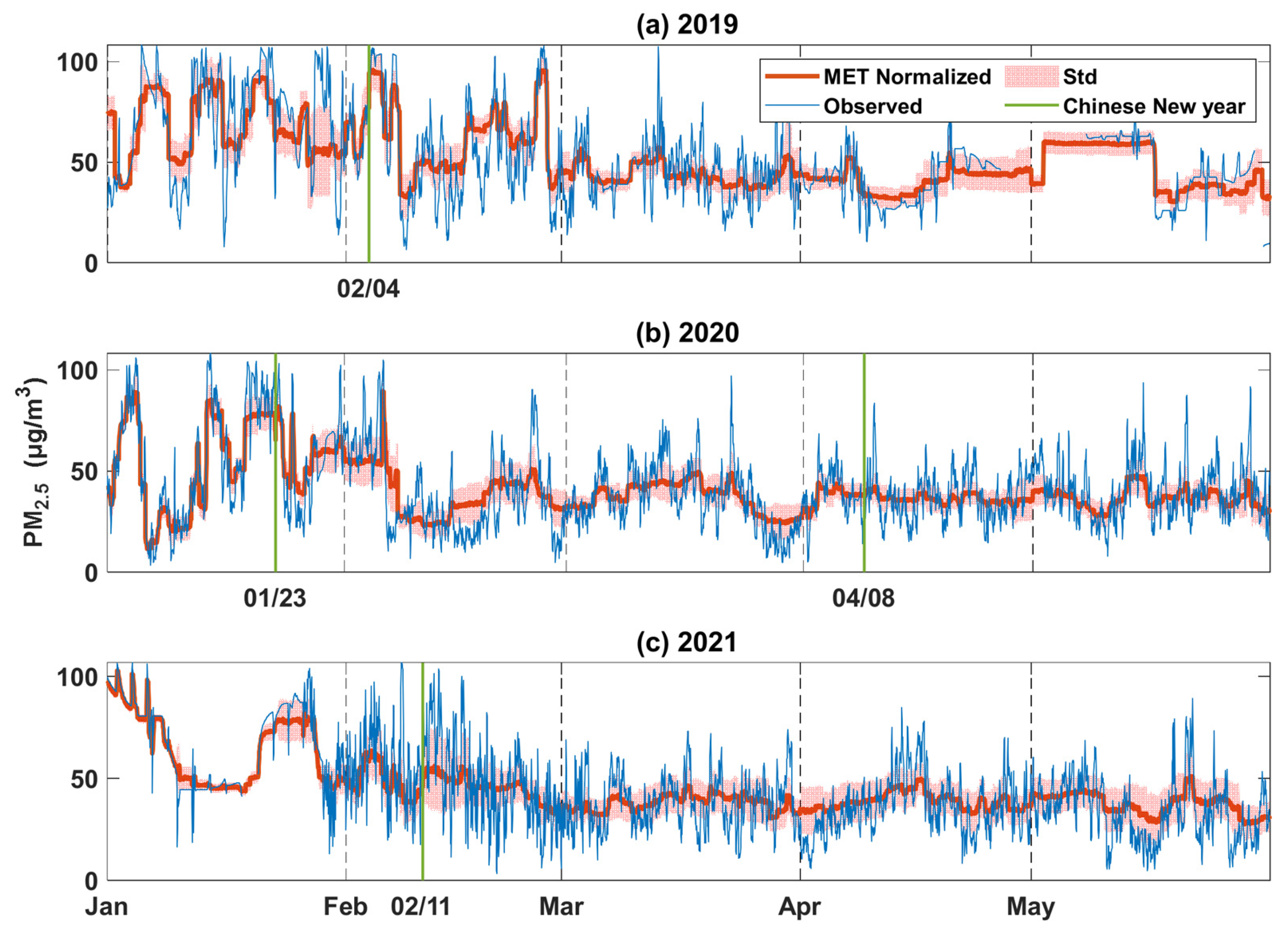
3.2.1. Time Series of Six Pollutants after Meteorological Normalization

The daily variation of PM2.5 concentrations before (in blue lines) and after (in thickened orange lines) meteorological normalization from January to May for the three years is shown in Figure 5. Before the lockdown year, there was a peak in anthropogenic PM2.5 emissions during the week of the Chinese Lunar New Year holiday in 2019, followed by a rapid decrease after the holiday. However, on 23 January 2020, which was also Chinese Lunar New Year’s Eve, the COVID-19 lockdown in Wuhan led to a significant reduction in PM2.5 levels. Despite the city being unlocked on 8 April 2020, anthropogenic PM2.5 concentrations remained relatively low for a long period. Comparably, in 2021, PM2.5 concentrations showed a slight increase after Lunar New Year’s Eve but remained at a low level because the government encouraged residents to stay at home during the Spring Festival, resulting in human activities not returning to the pre-lockdown level.
Annual variations of six pollutants after meteorological normalization are shown in Table 2 and Figure 6. Sharp decreases in anthropogenic pollutant concentrations can be observed during the lockdown (except for O3), with the ranking of NO2 > PM10 > SO2 > CO > PM2.5. Of the four gaseous pollutants, the concentration of NO2 decreased by 52%, from 50.90 μg/m3 in 2019 to 24.43 μg/m3 in 2020, followed by SO2 with a decrease of 31% and CO by 22%. Coal combustion is the primary source of NOx, SO2, and PM emissions, which are mainly produced by industrial activities such as power generation, cement and steel production, oil refining, and industrial boiler manufacturing [32]. The lockdown policy in the year 2020 required the shutting off of these plants, causing a significant decrease in pollution levels of NO2, SO2, and PM. In addition, road traffic control during the lockdown resulted in an additional constraint in NO2 emission [33], so the decrease in NO2 concentrations is prominently higher than that of SO2. Since nitrogen oxides (NOx) are the primary precursor of urban O3, the significant decrease in NOx during the lockdown resulted in a reduction in O3 consumption through titration (NO + O3→NO2 + O2), leading to an increase in O3 concentration [34,35,36].
Table 2 and Figure 6 also show that the concentrations of most anthropogenic pollutants rebounded in the post-lockdown year 2021, although they were still lower than before the pandemic. Notice that the concentration of man-made CO continued to decline over the observed three years. Fossil fuel consumption in the industrial and residential sectors is the primary source of CO emissions [32]. The unrecovered anthropogenic pollution level of CO indicates that industrial and residential processes remained depressed despite the reopening of industrial plants and residents’ lives in 2021. In addition, taking pollution levels in 2019 as a reference, PM10 decreased by 37% in 2020, which is 1.8 times greater than that of PM2.5 (21%). It rose by 40% in 2021, which is four times greater than that of PM2.5. Although PM2.5 and PM10 have many of the same sources of emissions, the change in PM10 during the locked and post-locked periods is significantly greater than that of PM2.5, primarily due to variations in road dust and construction activities [34].
Figure 7 shows the monthly variation of the human-associated six pollutants. SO2 concentration was higher in January and lower from February to May. The concentration decreased during the epidemic year and recovered somewhat after the epidemic, especially in March and April, which indicates activities of the burning of fossil fuel in stationary industrial factories and industrial processes. The strict city lockdown and road traffic controls implemented from 23 January to 8 April 2020 resulted in the lowest anthropogenic NO2 concentration during February and March of that year.
NO2 and O3 show opposite patterns of variation (Figure 7b,d). In the VOC-limited regime (the concentration VOC/NOx is relatively low), as generally reported in the urban area, low NO2 concentration leads to a low radical sink and would increase the chain reactions to generate O3. As a result, lower NO2 concentrations in cities are often accompanied by high O3 concentrations. Notice that the lowest NO2 in February 2020 did not correspond to the highest O3 concentration. This is because the NOx concentration drops sharply, making the VOC/NOx value large, and the O3 production enters the NOx-limited mode. Thus, the O3 concentration decreases with decreasing NOx [36]. In addition, the rapid reduction of PM (Figure 7e,f) suggests a decrease in the deposition of hydroperoxyl radicals, which can accelerate O3 production and lead to high O3 concentrations from February to April [37,38]. Atmospheric CO concentrations are highest in January (Figure 7c), mainly due to vehicle cold starts and decreased fuel combustion efficiency during the winter [39]. Compared to the pre-lockdown and lockdown years, CO concentrations are lowest from March to May in post-lockdown. This might come from further reducing incomplete petrochemical combustion, home heating, waste incineration, and domestic cooking [40].
To further evaluate the relationship between the pollutants and anthropogenic emission sources, we introduced the emission source inventory data MEIC (Multi-resolution Emission Inventory model for Climate and air pollution research) provided by the Tsinghua University team (the data were last updated in 2020) [32,41]. This dataset gives a monthly list of emission sources of pollutants from the five major departments, including agriculture, industry, power, residential, and transportation, at the 0.25° grid in China. The Figure 8 bar chart shows the changes in five emission sources of four pollutants, SO2, NOx, PM10, and PM2.5, in Wuhan from January to May 2019, with total emissions normalized to 1. The two lines in each subplot represent the monthly change in total anthropogenic emissions for 2019 and 2020. In general, the monthly changes in pollutants (Figure 7) are consistent with the total emission source changes (2019 red and 2020 pale blue lines in Figure 8) of the corresponding pollutants. The main anthropogenic emission sources of SO2 and PM are residential and industrial sources. The decrease in anthropogenic pollutants from January through April was primarily due to reductions in residential emissions. The main sources of NOx are industrial and transportation. As a large number of people stayed home for the New Year holidays in February 2019, this resulted in a low traffic emission of NOx in February. Ultimately, the human emissions in 2020 are all lower than in the same months in 2019. With the epidemic lockdown of Wuhan in February 2020, there is a steeper decline in the February 2020 anthropogenic emissions, which is consistent with the February folded point in Figure 7a,b,d,f).

3.2.2. Impact Variations of Meteorology and Anthropogenic Emissions on Six Pollutants

To better distinguish and measure the impact of human and weather factors on the annual variations of six pollutants, the changes in their observations (Obs) and predicted anthropogenic emissions (EMI), as well as the concentration changes induced by human beings (∆EMI) and meteorology (∆MET), are studied (Figure 9). Except for O3, anthropogenic and meteorological effects play opposite roles in the variation of pollutants, denoted by the orange and yellow bars. The EMIs (the orange lines) closely follow the changes in observation values (the blue lines), indicating that human activities play quite a dominant role in the changes in the local atmospheric environment.
The city lockdown intervention has resulted in a significant reduction in pollutant concentrations, offsetting the potential increase caused by weather conditions. As seen in Figure 9a, the SO2 observations decreased by 2.53 μg/m3 in the lockdown of 2020 compared to that of the pre-lockdown of 2019 (5.99 μg/m3 v.s. 8.53 μg/m3). The anthropogenic emission reduction contributed 89% to the total decrease, while the meteorology enhanced the concentration of SO2 by approximately 11% change. In the post-lockdown year of 2021, the SO2 concentration increased by 0.99 μg/m3, with an increase of 70% in anthropogenic emissions and a decrease of 30% due to weather alteration. A similar situation is shown for NO2, PM10, and PM2.5 as well. For CO, the decrease in observation of lockdown year is overwhelmingly anthropogenic (99% contribution), while in 2021, the concentration increases very slightly as a result of a combination of attenuated anthropogenic decrease and an enhanced promotion caused by weather conditions.
The increase in O3 concentration in the lockdown year results from both anthropogenic (69%) and meteorological contributions (31%) lift, while the decrease in the post-lockdown year is more contributed by meteorological conditions (−82%) (Figure 9d). For O3, the contribution of meteorology to the changes is greater than that of other pollutants, which suggests that the O3 variations are highly sensitive to changes in meteorology [27]. The future control measures for O3 pollution prevention should be considered in terms of both emission control and meteorological-related treatment.

3.2.3. Analysis of Atmospheric Oxidation and Aerosol Secondary Generation

Whether the reduction of gas pollutants in lockdown enhances atmospheric oxidation and secondary aerosol production is of interest to researchers to explain pollutant formation and evolution for sustainable urban environments. To verify the variations of secondary aerosol formation and atmospheric oxidation, the ratio changes in Ox, PM2.5/CO, NOR, and SOR for 2020/2019 and 2021/2019 are analyzed. Ox represents the ability of atmospheric oxidation to generate secondary gases NO2 and O3. Among them, urban NO2 is mainly produced by the atmospheric oxidation of NO emitted from vehicle exhaust. The formation of near-surface O3 through photochemical reactions is dependent on the emissions of NOx and VOCs [36]. PM2.5/CO represents the strength of secondary generation relative to initial emissions, while SOR and NOR represent the generation of secondary sulfate and nitrate. Figure 10a shows that the Ox (O3 + NO2) atmospheric oxidation capacity is weaker in the lockdown year than the pre-lockdown year (Ox2020/2019 < 1), except for a few hours around 17:00. This is mainly caused by the unnatural drop of NO2 (Figure 10b), and O3 concentrations are elevated due to O3–VOC–NOx relationships [42,43]. The concentration of Ox decreases even more during the post-lockdown period (below the 1:1 line), which is the joint result of a large retreat of O3 and a small recovery of NO2. In addition, the Ox ratio shows a clear trend of diurnal variation. It decreases to low levels between midnight and around 7:00 a.m. LT, after which it starts to rise and reaches its maximum at approximately 5:00 p.m. LT. The lower morning concentrations may be attributed to the depositional loss of Ox under stable atmospheric conditions in the early morning hours. The afternoon peak in Ox concentration is likely due to the accumulation of local photochemical reactions under weak solar radiation [44].
The PM2.5/CO ratio can serve as an index of secondary formation versus primary emission because CO is primarily emitted through primary sources, while PM2.5 is a mixture of primary and secondary aerosols [9]. Figure 10b shows that the PM2.5/CO ratio in the lockdown year is moderately smaller than in the pre-lockdown year (PM2.5/CO(2020/2019) < 1). In post-lockdown, the secondary formation ratio is larger than in lockdown (above the 1:1 line) but is not recovered to the pre-lockdown level (PM2.5/CO(2021/2019) varies around the value of 1), which is only slightly higher in 8:00–10:00 a.m. LT, 6:00–9:00 p.m. LT. This indicates that the atmospheric secondary formation in post-lockdown is weakly higher than in pre-lockdown during rush hours and lower at other hours.
For SOR and NOR (Figure 10c,d), SOR2020/2019 is smaller than 1 during the daytime (8:00 a.m.–8:00 p.m. LT) and larger than 1 at night (8:00 p.m.–8:00 a.m. LT), indicating a higher sulfate generation efficiency at night and lower efficiency in the daytime in 2020. The primary cause of the lower SOR during the day is the substantial reduction in SO2 precursor gas emissions that occurred during the lockdown year. The increased SO2 to sulfate conversion throughout the night is probably due to nocturnal aqueous-phase chemical processes [45]. In the lockdown year 2020, during most hours of the day, the NOR is slightly higher than pre-lockdown levels, except for a few hours around midnight. This deviation may be attributed to photochemical reactions occurring under the conditions of high O3 concentrations and solar radiation [44]. In contrast, the 2021/2019 ratios for both NOR and SOR are higher than 1 and are also higher than that of 2020/2019 (above the 1:1 line), indicating the stronger sulfate and nitrate formation in the post-lockdown year.

4. Conclusions

To quantify the pollutant changes due to anthropogenic emissions contributing to sustainable urban development, this study separated the observed pollutant concentrations into meteorological and anthropogenic emissions and analyzed their changes from 2019 to 2021 (1 January to 31 May). The main findings are summarized as follows:
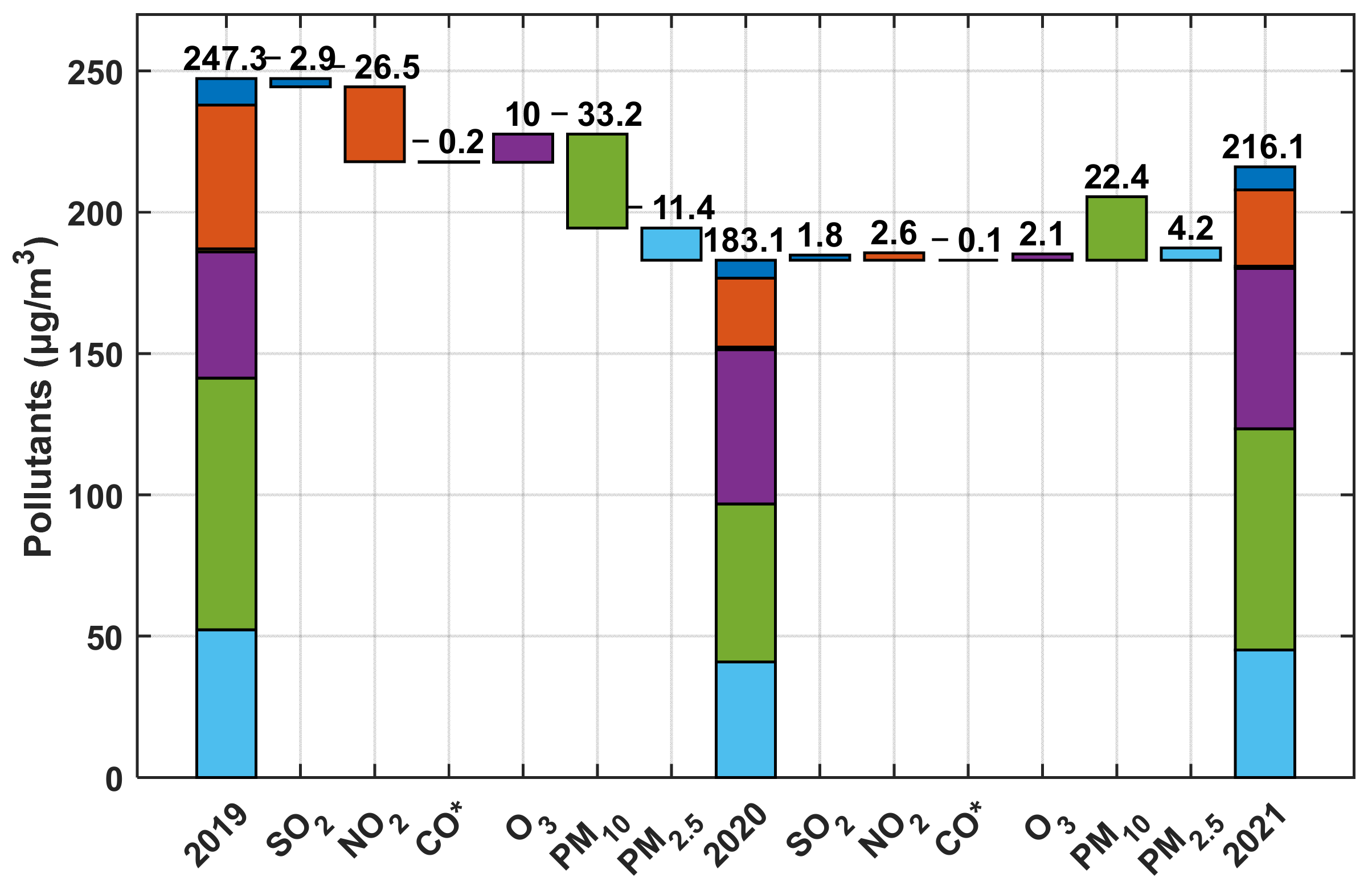
  • The peak of anthropogenic pollutants in the Chinese Lunar New Year festival was significantly reduced in 2020 due to the lockdown and remained at low levels during the same period in post-lockdown year 2021. Sharp decreases in anthropogenic pollutants can be observed during lockdown (except for O3), and the rankings are NO2 > PM10 > SO2 > CO > PM2.5.
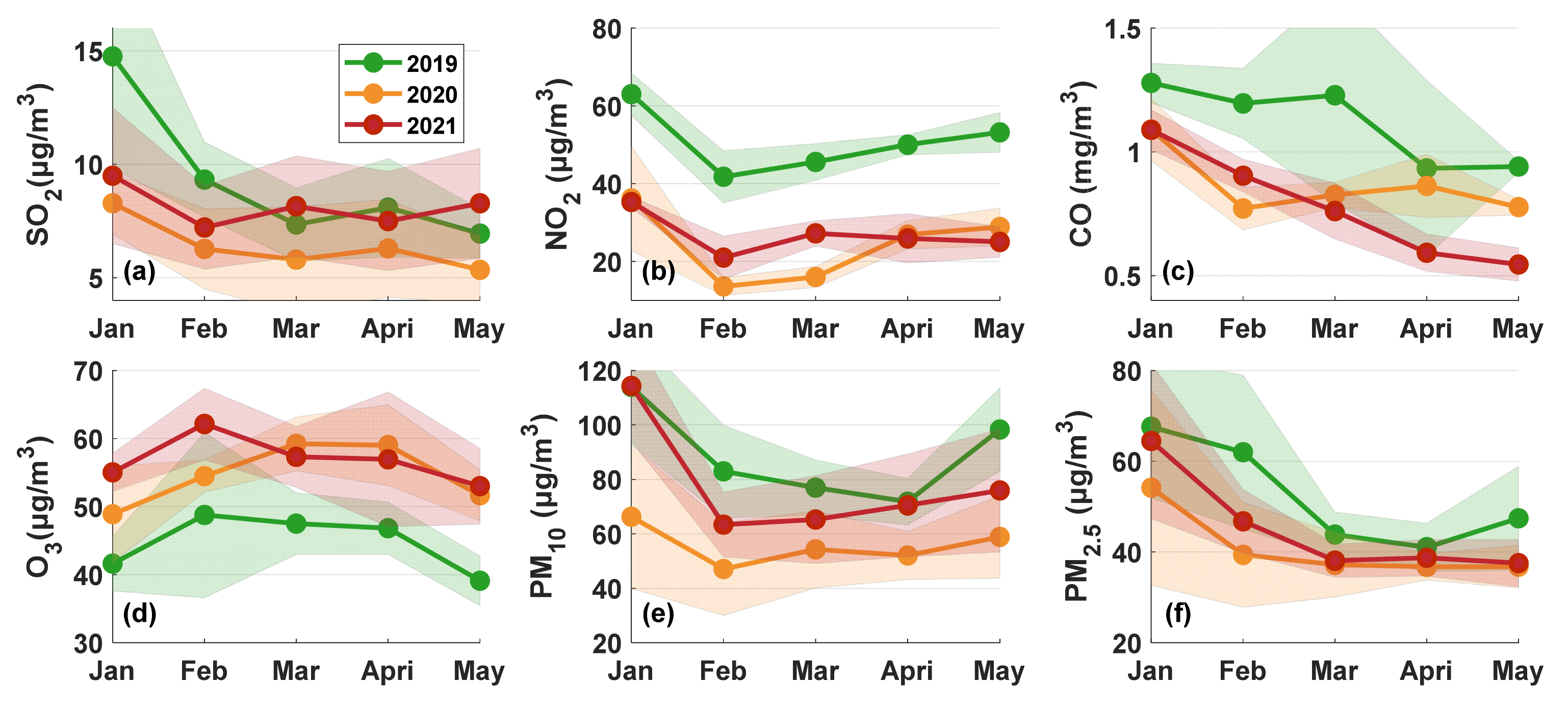
  • The pre- and post-lockdown years exhibit large monthly variations in all six pollutants, whereas the lockdown period shows a small monthly fluctuation in these pollutants. The lowest anthropogenic NO2 concentration appears in February and March during the lockdown, which is a clear indication of the severe city closure and road traffic controls. The lower concentration of NO2 led to a low efficiency of O3 consumption and brought about high concentrations of O3 from February to April 2020.
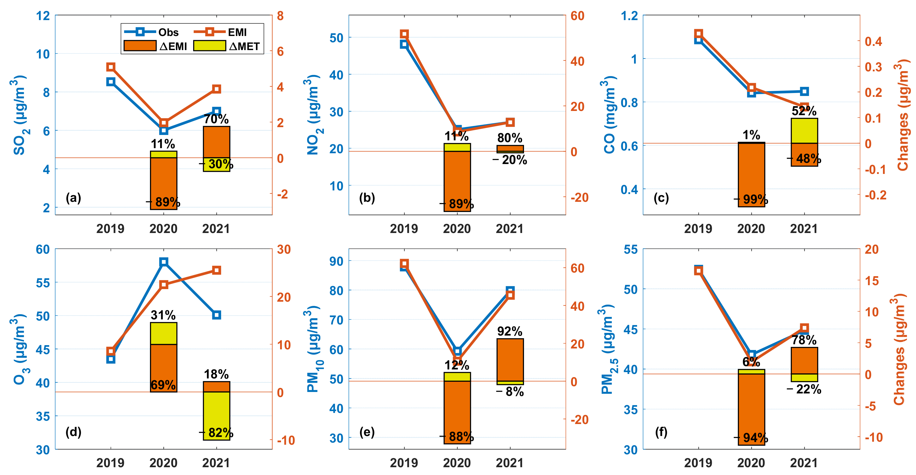
  • Anthropogenic and meteorological factors have opposing effects on the variation of pollutants, but anthropogenic factors appear to be dominant. The significant reduction in human activities has led to a sharp decrease in pollutant concentrations and has counteracted any potential increase caused by weather conditions. Of all six pollutants, O3 is the one that is relatively least subject to anthropogenic emissions.
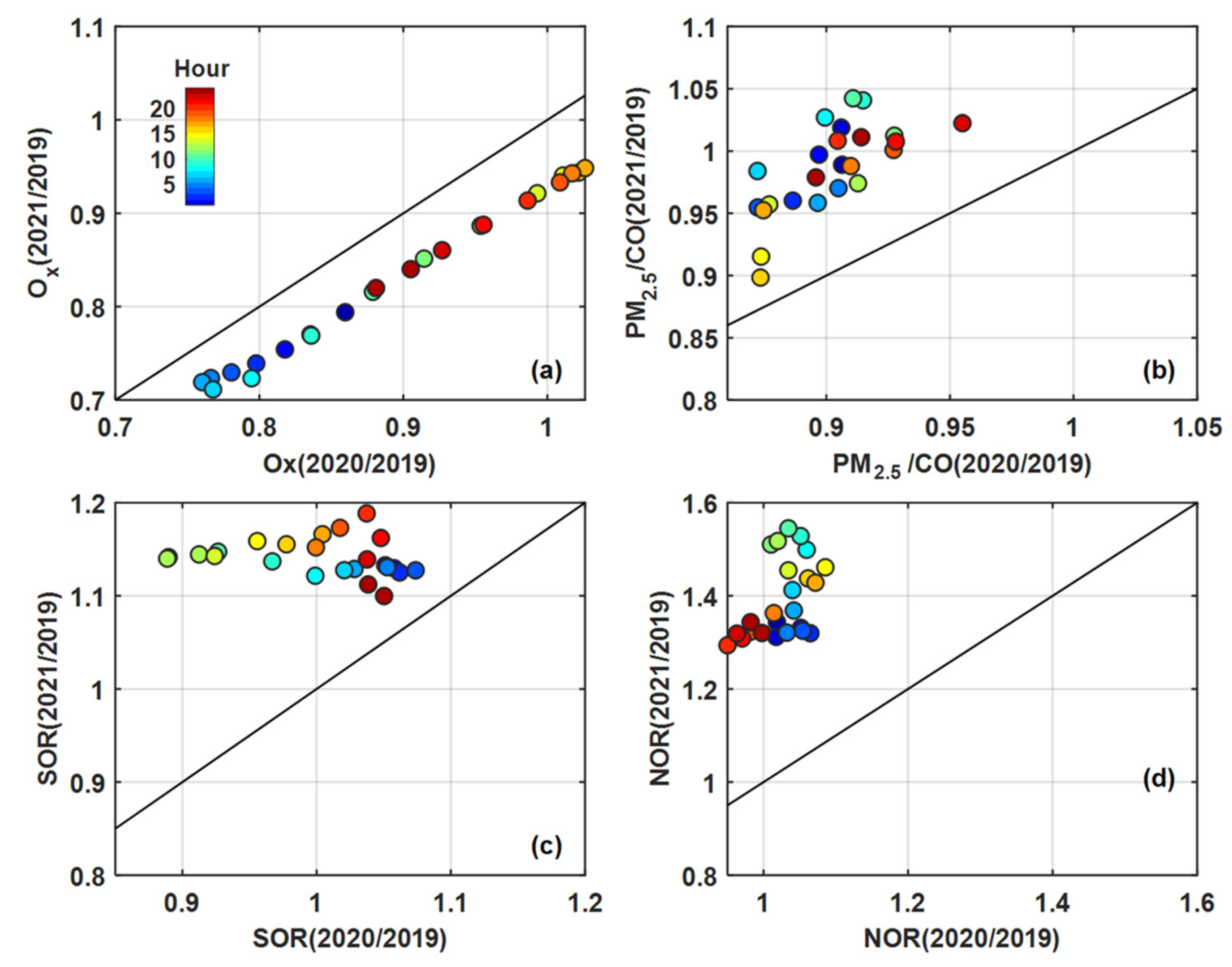
  • The atmospheric oxidation capacity of Ox, the PM2.5/CO ratio, and SOR in the lockdown year were lower than pre-lockdown levels, while NOR increased slightly for most hours of the day, attributed to the relatively high O3 and sharply low NO2. In the post-epidemic year, the PM2.5/CO secondary production and the generation of sulfate and nitrate were stronger than in the pre-lockdown period, while Ox was weakened, which was the joint result of a large retreat of O3 and a small recovery of NO2.

Author Contributions

Methodology and software: Y.Z.; Conceptualization and methodology: J.C.; Writing—original draft: Y.Z.; Resources: J.S. and B.Z.; Validation and supervision: J.C.; Validation and software: M.D. All authors have read and agreed to the published version of the manuscript.

Funding

This work was supported by the National Key R&D Program of China (No. 2023YFF0611904), and the Open Fund of Key Laboratory of National Geographical Census and Monitoring, Ministry of Natural Resources (No. 2022NGCM02).

Institutional Review Board Statement

Not applicable.

Informed Consent Statement

Not applicable.

Data Availability Statement

Available upon reasonable request from the corresponding authors.

Acknowledgments

Our gratitude goes to the Hubei Eco-Environmental Monitoring Centre for furnishing us with the in -situ observation data.

Conflicts of Interest

The authors declare no conflict of interest.

References

  1. Lv, Y. Tempo-Spatial Characteristics of Air Quality in Wuhan and the Influence of Meteorological Parameters; Huazhong Agricultural University: Wuhan, China, 2019. (In Chinese) [Google Scholar]
  2. You, M. Addition of PM2.5 into the National Ambient Air Quality Standards of China and the Contribution to Air Pollution Control: The Case Study of Wuhan, China. Sci. World J. 2014, 2014, 768405. [Google Scholar] [CrossRef] [PubMed]
  3. Shen, L.; Zhao, T.; Wang, H.; Liu, J.; Bai, Y.; Kong, S.; Zheng, H.; Zhu, Y.; Shu, Z. Importance of meteorology in air pollution events during the city lockdown for COVID-19 in Hubei Province, Central China. Sci. Total Environ. 2021, 754, 142227. [Google Scholar] [CrossRef]
  4. Jiang, S.; Kong, S.; Zheng, H.; Zeng, X.; Chen, N.; Qi, S. Real-time source apportionment of PM2.5 and potential geographic origins of each source during winter in Wuhan. Environ. Sci. 2022, 43, 61–73. (In Chinese) [Google Scholar]
  5. Grange, S.K.; Carslaw, D.C. Using meteorological normalisation to detect interventions in air quality time series. Sci. Total Environ. 2019, 653, 578–588. [Google Scholar] [CrossRef] [PubMed]
  6. Chen, N.; Zhang, Z.; Tao, L.; Bo, Z.; Ke, X.; Cao, W.; Ding, Q.; Bo, L.; Wang, L.; Li, Y. Air quality change and improvement measures during the COVID-19 epidemic in Wuhan. Clim. Environ. Res. 2021, 26, 217–226. (In Chinese) [Google Scholar]
  7. Yao, L.; Kong, S.; Zheng, H.; Chen, N.; Zhu, B.; Xu, K.; Cao, W.; Zhang, Y.; Zheng, M.; Cheng, Y. Co-benefits of reducing PM2.5 and improving visibility by COVID-19 lockdown in Wuhan. NPJ Clim. Atmos. Sci. 2021, 4, 40. [Google Scholar] [CrossRef]
  8. Huang, Z.; Kong, S.; Chen, N.; Yan, Y.; Liu, D.; Zhu, B.; Xu, K.; Cao, W.; Ding, Q.; Lan, B.; et al. Significant changes in the chemical compositions and sources of PM2.5 in Wuhan since the city lockdown as COVID-19. Sci. Total Environ. 2020, 739, 140000. [Google Scholar]
  9. Huang, X.; Ding, A.; Gao, J.; Zheng, B.; Zhou, D.; Qi, X.; Tang, R.; Wang, J.; Ren, C.; Nie, W.; et al. Enhanced secondary pollution offset reduction of primary emissions during COVID-19 lockdown in China. Natl. Sci. Rev. 2021, 8, nwaa137. [Google Scholar] [CrossRef]
  10. Lu, S.; Shi, X.; Xue, W.; Yu, L.; Gang, Y. Impacts of Meteorology and Emission Variations on PM2.5 Concentration Throughout the Country during the 2020 Epidemic Period. Environ. Sci. 2021, 42, 3099–3106. (In Chinese) [Google Scholar]
  11. Zhou, Y.; Zhu, K.; Fan, H.; Dan, L.; Wei, L. Emission reductions and air quality improvements during the COVID-19 pandemic in Hubei province. Environ. Sci. Technol. 2020, 43, 228–236. (In Chinese) [Google Scholar]
  12. Zareba, M.; Dlugosz, H.; Danek, T.; Weglinska, E. Big-Data-Driven Machine Learning for Enhancing Spatiotemporal Air Pollution Pattern Analysis. Atmosphere 2023, 14, 760. [Google Scholar] [CrossRef]
  13. Grange, S.K.; Carslaw, D.C.; Lewis, A.C.; Boleti, E.; Hueglin, C. Random forest meteorological normalisation models for Swiss PM 10 trend analysis. Atmos. Chem. Phys. 2018, 18, 6223–6239. [Google Scholar] [CrossRef]
  14. Qu, L.; Liu, S.; Ma, L.; Zhang, Z.; Du, J.; Zhou, Y.; Meng, F. Evaluating the meteorological normalized PM2.5 trend (2014–2019) in the “2 + 26” region of China using an ensemble learning technique. Environ. Pollut. 2020, 266, 115346. [Google Scholar] [CrossRef] [PubMed]
  15. The State Council of China. Air Pollution Prevention and Control Action Plan. Available online: http://www.gov.cn/zwgk/2013-09/12/content_2486773.htm (accessed on 1 September 2023). (In Chinese)
  16. Zhang, L.; Qian, J.; Du, Y.; Nan, W.; Yi, J.; Sun, Y.; Ting, M.; Tao, P.; Zhou, C. Multi-level spatial distribution estimation model of the inter- regional migrant population using multi- source spatio-temporal big data: A case study of migrants from Wuhan during the spread of COVID-19. J. Geo-Inf. Sci. 2020, 22, 147–160. (In Chinese) [Google Scholar]
  17. Pang, Y.; Li, Y.; Lu, M.; Lu, Z.; Zhou, L. Analysis of the spatio-temporal process and humanistic influencing factors of COVID-19 spread in Hubei Province. J. Cap. Norm. Univ. (Nat. Sci. Ed.) 2022, 43, 53–62 + 87. (In Chinese) [Google Scholar]
  18. Liu, H.; Yue, F.; Xie, Z. Quantify the role of anthropogenic emission and meteorology on air pollution using machine learning approach: A case study of PM2.5 during the COVID-19 outbreak in Hubei Province, China. Environ. Pollut. 2022, 300, 118932. [Google Scholar] [CrossRef] [PubMed]
  19. Hastie, T.; Tibshirani, R.; Friedman, J.H. The Elements of Statistical Learning: Data Mining, Inference, and Prediction, 2nd ed.; Springer: Berlin/Heidelberg, Germany, 2009; Volume 2, p. 767. [Google Scholar]
  20. Zhai, S.; Jacob, D.J.; Wang, X.; Shen, L.; Li, K.; Zhang, Y.; Gui, K.; Zhao, T.; Liao, H. Fine particulate matter (PM2.5) trends in China, 2013–2018: Separating contributions from anthropogenic emissions and meteorology. Atmos. Chem. Phys. 2019, 19, 11031–11041. [Google Scholar] [CrossRef]
  21. Zhu, B.; Zhang, Y.; Chen, N.; Quan, J. Assessment of Air Pollution Aggravation during Straw Burning in Hubei, Central China. Int. J. Environ. Res. Public Health 2019, 16, 1446. [Google Scholar] [CrossRef]
  22. Fu, Q.; Zhuang, G.; Wang, J.; Xu, C.; Huang, K.; Li, J.; Hou, B.; Lu, T.; Streets, D.G. Mechanism of formation of the heaviest pollution episode ever recorded in the Yangtze River Delta, China. Atmos. Environ. 2008, 42, 2023–2036. [Google Scholar] [CrossRef]
  23. Li, X.; Wang, L.; Ji, D.; Wen, T.; Pan, Y.; Sun, Y.; Wang, Y. Characterization of the size-segregated water-soluble inorganic ions in the Jing-Jin-Ji urban agglomeration: Spatial/temporal variability, size distribution and sources. Atmos. Environ. 2013, 77, 250–259. [Google Scholar] [CrossRef]
  24. Pierson, W.R.; Brachaczek, W.W.; Mckee, D.E. Sulfate Emissions from Catalyst-Equipped Automobiles on the Highway. J. Air Pollut. Control Assoc. 1979, 29, 255–257. [Google Scholar] [CrossRef]
  25. Choi, W.; Ho, C.-H.; Kim, K.-Y. Critical contribution of moisture to the air quality deterioration in a warm and humid weather. Sci. Rep. 2023, 13, 4260. [Google Scholar] [CrossRef] [PubMed]
  26. De Gouw, J.A.; Welsh-Bon, D.; Warneke, C.; Kuster, W.; Alexander, L.; Baker, A.K.; Beyersdorf, A.J.; Blake, D.; Canagaratna, M.; Celada, A. Emission and chemistry of organic carbon in the gas and aerosol phase at a sub-urban site near Mexico City in March 2006 during the MILAGRO study. Atmos. Chem. Phys. 2009, 9, 3425–3442. [Google Scholar] [CrossRef]
  27. Dang, R.; Liao, H.; Fu, Y. Quantifying the anthropogenic and meteorological influences on summertime surface ozone in China over 2012–2017. Sci. Total Environ. 2021, 754, 142394. [Google Scholar] [CrossRef] [PubMed]
  28. Cao, J.; Shen, Z.; Chow, J.C.; Watson, J.G.; Lee, S.; Tie, X.; Ho, K.; Wang, G.; Han, Y. Winter and Summer PM2.5 Chemical Compositions in Fourteen Chinese Cities. J. Air Waste Manag. Assoc. 2012, 62, 1214–1226. [Google Scholar] [CrossRef] [PubMed]
  29. Sun, Y.L.; Wang, Z.F.; Fu, P.Q.; Yang, T.; Jiang, Q.; Dong, H.B.; Li, J.; Jia, J.J. Aerosol composition, sources and processes during wintertime in Beijing, China. Atmos. Chem. Phys. 2013, 13, 4577–4592. [Google Scholar] [CrossRef]
  30. Bressi, M.; Sciare, J.; Ghersi, V.; Mihalopoulos, N.; Petit, J.E.; Nicolas, J.B.; Moukhtar, S.; Rosso, A.; Féron, A.; Bonnaire, N.; et al. Sources and geographical origins of fine aerosols in Paris (France). Atmos. Chem. Phys. 2014, 14, 8813–8839. [Google Scholar] [CrossRef]
  31. Trebs, I.; Meixner, F.X.; Slanina, J.; Otjes, R.; Jongejan, P.; Andreae, M.O. Real-time measurements of ammonia, acidic trace gases and water-soluble inorganic aerosol species at a rural site in the Amazon Basin. Atmos. Chem. Phys. 2004, 4, 967–987. [Google Scholar] [CrossRef]
  32. Li, M.; Liu, H.; Geng, G.; Hong, C.; Liu, F.; Song, Y.; Tong, D.; Zheng, B.; Cui, H.; Man, H.; et al. Anthropogenic emission inventories in China: A review. Natl. Sci. Rev. 2017, 4, 834–866. [Google Scholar] [CrossRef]
  33. Zhou, J.; Yu, H.; Peipei, Q.; Hao, L.; Kai, X. Air pollutant emission inventory and distribution characteristics in Wuhan city. J. Nanjing Univ. Inf. Sci. Technol. (Nat. Sci. Ed.) 2018, 10, 599–605. (In Chinese) [Google Scholar]
  34. Tobías, A.; Carnerero, C.; Reche, C.; Massagué, J.; Via, M.; Minguillón, M.C.; Alastuey, A.; Querol, X. Changes in air quality during the lockdown in Barcelona (Spain) one month into the SARS-CoV-2 epidemic. Sci. Total Environ. 2020, 726, 138540. [Google Scholar] [CrossRef]
  35. Li, H.; Wang, D.; Cui, L.; Gao, Y.; Huo, J.; Wang, X.; Zhang, Z.; Tan, Y.; Huang, Y.; Cao, J. Characteristics of atmospheric PM2.5 composition during the implementation of stringent pollution control measures in shanghai for the 2016 G20 summit. Sci. Total Environ. 2019, 648, 1121–1129. [Google Scholar] [CrossRef] [PubMed]
  36. Jenkin, M.E.; Clemitshaw, K.C. Ozone and other secondary photochemical pollutants: Chemical processes governing their formation in the planetary boundary layer. In Developments in Environmental Science; Austin, J., Brimblecombe, P., Sturges, W., Eds.; Elsevier: London, UK, 2002; Volume 1, pp. 285–338. [Google Scholar]
  37. Xu, W.; Liu, X.; Liu, L.; Dore, A.; Tang, A.-H.; Lu, L.; Wu, Q.-M.; Zhang, Y.; Hao, T.; Pan, Y.; et al. Impact of emission controls on air quality in Beijing during APEC 2014: Implications from water-soluble ions and carbonaceous aerosol in PM2.5 and their precursors. Atmos. Environ. 2019, 210, 241–252. [Google Scholar] [CrossRef]
  38. Li, K.; Jacob, D.J.; Liao, H.; Shen, L.; Zhang, Q.; Bates, K.H. Anthropogenic drivers of 2013–2017 trends in summer surface ozone in China. Proc. Natl. Acad. Sci. USA 2019, 116, 422–427. [Google Scholar] [CrossRef] [PubMed]
  39. Helfter, C.; Tremper, A.H.; Halios, C.H.; Kotthaus, S.; Bjorkegren, A.; Grimmond, C.S.B.; Barlow, J.F.; Nemitz, E. Spatial and temporal variability of urban fluxes of methane, carbon monoxide and carbon dioxide above London, UK. Atmos. Chem. Phys. 2016, 16, 10543–10557. [Google Scholar] [CrossRef]
  40. Jaffe, L.S. Carbon monoxide in the biosphere: Sources, distribution, and concentrations. J. Geophys. Res. 1973, 78, 5293–5305. [Google Scholar] [CrossRef]
  41. Zheng, B.; Tong, D.; Li, M.; Liu, F.; Hong, C.; Geng, G.; Li, H.; Li, X.; Peng, L.; Qi, J. Trends in China’s anthropogenic emissions since 2010 as the consequence of clean air actions. Atmos. Chem. Phys. 2018, 18, 14095–14111. [Google Scholar] [CrossRef]
  42. Liu, T.; Hong, Y.; Li, M.; Xu, L.; Chen, J.; Bian, Y.; Yang, C.; Dan, Y.; Zhang, Y.; Xue, L.; et al. Atmospheric oxidation capacity and ozone pollution mechanism in a coastal city of southeastern China: Analysis of a typical photochemical episode by an observation-based model. Atmos. Chem. Phys. 2022, 22, 2173–2190. [Google Scholar] [CrossRef]
  43. Wang, M.; Chen, W.; Zhang, L.; Qin, W.; Zhang, Y.; Zhang, X.; Xie, X. Ozone pollution characteristics and sensitivity analysis using an observation-based model in Nanjing, Yangtze River Delta Region of China. J. Environ. Sci. 2020, 93, 13–22. (In Chinese) [Google Scholar] [CrossRef]
  44. Meng, Z.; Xu, X.; Lin, W.; Ge, B.; Xie, Y.; Song, B.; Jia, S.; Zhang, R.; Peng, W.; Wang, Y.; et al. Role of ambient ammonia in particulate ammonium formation at a rural site in the North China Plain. Atmos. Chem. Phys. 2018, 18, 167–184. [Google Scholar] [CrossRef]
  45. Wang, Y.; Li, Z.; Wang, Q.; Jin, X.; Yan, P.; Cribb, M.; Li, Y.; Yuan, C.; Wu, H.; Wu, T.; et al. Enhancement of secondary aerosol formation by reduced anthropogenic emissions during Spring Festival 2019 and enlightenment for regional PM2.5 control in Beijing. Atmos. Chem. Phys. 2021, 21, 915–926. [Google Scholar] [CrossRef]
Figure 1. The map of the sampling location (the red cross) in Wuhan, Hubei Province, China. Wuhan is a 10-million-population industrial city in central China, where ambient air quality is strongly influenced by meteorological variations and anthropogenic emissions.
Sustainability 15 16694 g001
Figure 2. The diagram of the analysis model and meteorological normalization. Each data record Xi (I = 1, …, N; here, N = 10,895) contains 4 temporal (Times, including Julian day, DOY, DOM, and weekday), 5 meteorological variables (METs, including WS, WD, T, RH, and P), and 6 pollutant variables Yij (j = 1, 2, 3, 4, 5, 6). Xi(1~1000) and Yij(1~1000) are the renewed input vectors with random meteorology and corresponding predictions, which are repeated 1000 times.
Sustainability 15 16694 g002
Figure 3. Importance of meteorology parameters on five pollutants (a) SO2, (b) NO2, (c) CO, (d) PM2.5, (e) O3 in the boosted regression tree model and their linear correlation (f).
Sustainability 15 16694 g003
Figure 4. PM2.5 distribution on time and meteorological variables: (a) Julian day, (b) DOY, (c) DOM, (d) weekday, (e) WD (wind direction), (f) WS (wind speed), (g) T (temperature), (h) RH (relative humidity), (i) P (pressure).
Sustainability 15 16694 g004
Figure 5. Observation (Observed) and meteorologically normalized (MET Normalized) PM2.5 concentrations from 1 January to 31 May over the three years: (a) 2019, (b) 2020, (c) 2021. The red shaded area represents the model standard deviation range. The green vertical lines indicate Chinese Lunar New Year’s Eve. The first and second green lines in Panel (b) mark the beginning and the end of the city lockdown in Wuhan.
Sustainability 15 16694 g005
Figure 6. Annual variation of six pollutants after meteorological normalization (CO*, the * represents the concentration is in mg/m3).
Sustainability 15 16694 g006
Figure 7. Monthly variation of six pollutants after meteorological normalization before, during, and after the lockdown: (a) SO2, (b) NO2, (c) CO, (d) O3, (e) PM10, (f) PM2.5.
Sustainability 15 16694 g007
Figure 8. Monthly variation of five emission sources of four pollutants in Wuhan from January to May in 2019: (a) SO2, (b) NOx, (c) PM10, (d) PM2.5. The lines in each subplot represent the total anthropogenic emission changes of 2019 (red) and 2020 (pale blue).
Sustainability 15 16694 g008
Figure 9. Separation of pollutant observations (Obs) into anthropogenic emissions (EMI) and meteorological variations (MET): (a) SO2, (b) NO2, (c) CO, (d) O3, (e) PM10, (f) PM2.5. The broken lines represent the observation and EMI contributions, referred to the left y-axis. The stacked bars represent the changes in EMI (orange) and MET (yellow) relative to the previous year, referred to the right y-axis. The numbers on the bar represent the percentage of change.
Sustainability 15 16694 g009
Figure 10. Ratio changes of atmospheric oxidation properties for the lockdown (2020/2019) and post-lockdown (2021/2019) periods: (a) Ox oxidation (Ox = O3 + NO2), (b) PM2.5/CO, (c) secondary production of sulfate (SOR), (d) secondary production of nitrate (SNR).
Sustainability 15 16694 g010
Table 1. Parameters of the boosted regression tree model obtained by parametric self-optimization algorithm for six pollution covariates.
ResponsesNumber of Weak LearnersLearning RateMax. Number
of Splits
R2
SO24980.326430.998
NO24910.285960.990
CO4650.1044070.983
O34590.0971040.989
PM2.51770.1182720.998
PM101650.1836040.999
Table 2. Annual changes of six pollutants due to anthropogenic emissions (1 January to 31 May); each value is mean ± standard deviation.
Species2019
(Pre-)
(μg/m3)
2020
(Lockdown)
(μg/m3)
2021
(Post-)
(μg/m3)
2020
Relative to
2019
2021
Relative to
2020
SO29.30 ± 3.946.40 ± 2.118.15 ± 2.49−31 ± 17%27 ± 12%
NO250.90 ± 8.8424.43 ± 10.8227.03 ± 6.41−52 ± 25%11 ± 5%
CO* (mg/m3)1.12 ± 0.300.87 ± 0.150.78 ± 0.21−22 ± 7%−10 ± 3%
O344.67 ± 7.3854.63 ± 6.4056.78 ± 6.7522 ± 5%4 ± 0.6%
PM1089.03 ± 21.6155.85 ± 18.5078.24 ± 26.39−37 ± 15%40 ± 19%
PM2.552.26 ± 15.8540.90 ± 13.5145.13 ± 13.72−21 ± 10%10 ± 5%
Disclaimer/Publisher’s Note: The statements, opinions and data contained in all publications are solely those of the individual author(s) and contributor(s) and not of MDPI and/or the editor(s). MDPI and/or the editor(s) disclaim responsibility for any injury to people or property resulting from any ideas, methods, instructions or products referred to in the content.

