Ground-Level Particulate Matter (PM_2.5) Concentration Mapping in the Central and South Zones of Peninsular Malaysia Using a Geostatistical Approach

Abstract

Fine particulate matter is one of the atmospheric contaminants that exist in the atmosphere. The purpose of this study is to evaluate spatial–temporal changes in PM_2.5 concentrations in the central and south zones of Peninsular Malaysia from 2019 to 2020. The study area involves twenty-one monitoring stations in the central and south zones of Peninsular Malaysia, using monthly and annual means of PM_2.5 concentrations. The spatial autocorrelation of PM_2.5 is calculated using Moran’s I, while three semi-variogram models are used to measure the spatial variability of PM_2.5. Three kriging methods, ordinary kriging (OK), simple kriging (SK), and universal kriging (UK), were used for interpolation and comparison. The results showed that the Gaussian model was more appropriate for the central zone (MSE = 14.76) in 2019, while the stable model was more suitable in 2020 (MSE = 19.83). In addition, the stable model is more appropriate for both 2019 (MSE = 12.68) and 2020 (8.87) for the south zone. Based on the performance indicator, universal kriging was chosen as the best interpolation method in 2019 and 2020 for both the central and south zone. In conclusion, the findings provide a complete map of the variations in PM_2.5 for two different zones, and show that interpolation methods such as universal kriging are beneficial and could be extended to the investigation of air pollution distributions in other areas of Peninsular Malaysia.

1. Introduction

Air pollution is one of the biggest environmental concerns around the world [1]. Air pollution is mostly caused by meteorological factors, with PM_2.5 being the most dangerous pollutant [2]. Fine particulate matter has a negative effect on health and harms the body when we are exposed to it in the short and long term [3]. In 2013, the WHO’s International Agency for Research Cancer (IARC) identified particulate matter as a potential cause of lung cancer. Exposure to PM_2.5 can lead to breathing illnesses such as chronic obstructive pulmonary disease (CPPD) [4], acute lower respiratory tract infections, myocardial infarctions, and lung cancer [5,6], as well as other acute and chronic respiratory illnesses, heart disease, and strokes in both urban and rural regions. The levels of PM_2.5 and other pollutants emitted into the atmosphere have started to interfere with normal biological functions [7]. By emphasizing the significance of precise PM_2.5 prediction in health risk assessment and air pollution control, the study of PM_2.5 offers a scientific foundation for comprehending and preventing air pollution in different areas [8,9]. The major sources of PM_2.5 include biomass burning, industrial activities, and motor vehicles [10,11].

Urbanization and industry have been linked to air pollution; as a result, a lot of studies have been performed in cities in developed countries [12,13,14]. There are different classifications of zones, which include rural, suburban, urban, and industrial. The spatial distributions of air pollution, such as PM concentrations, in urban areas were higher than in rural areas of the same region [15]. Concentrations of particulate matter are influenced by weather and climate factors, since the movement and dispersion of air pollutants in the surrounding atmosphere are affected by wind patterns, vertical mixing, and precipitation. These processes lead to alterations in particulate matter such as PM_2.5 concentrations over space and time [16]. The rapid development of urban cities and the growth of the economy have accelerated the growth of the automobile industry as well as the rate at which vehicles are present in cities. In recent years, environmental pollution including PM_2.5 from motor vehicles has worsened [17,18]. Furthermore, it has been observed that PM_2.5 exhibits more favorable characteristics in high-income countries that have completed the stages of rapid urbanization and economic growth. Nevertheless, low- and middle-income nations are either experiencing, or are on the verge of, fast-paced urbanization and economic development, which poses a potential threat regarding the concentration of particulate matter [18].

Spatial autocorrelation is used to identify the correlations in data across location and time. Moran’s I evaluate the dispersion, unpredictability, or clustering of data patterns. Moran’s I is frequently used in geography and geographic information science (GIS) to assess how closely clustered certain map features are. A study by Zhang et al. [19] undertook spatial autocorrelation using Moran’s I and found that the air quality in 19 Chinese cities increased and decreased over the past six years, with winter pollution being more severe. The spatial autocorrelation of these changes showed similar trends across different regions, indicating an expansion trend in air pollution levels. Global and local Moran’s I were used to measure the spatial autocorrelation of the air quality index (AQI) values from thirteen cities in China. The study reveals that the air quality in Northern and Southern Jiangsu is better than in the central region, with Southern Jiangsu experiencing worse air quality in certain seasons and months [20]. A study in Poland by (Danek et al. 2022) [21], using a geostatistical approach (standardized geographical weighted regression (GWR), Moran 1, Getis-Ord Gi) on data from during the COVID-19 lockdown, found that topography, meteorological variables, and PM concentrations are related. The results revealed a correlation between meteorological factors and pollution, with higher PM₁₀ values linked to lower temperatures and higher relative humidity. Before estimating via kriging, it is important to produce the semi-variograms (exponential, spherical, stable, Gaussian model) to make sure the data meet these requirements. The model with the fewest residuals should be selected when modelling a variogram. A study by Tong et al. [22] described how the exponential model was the most suitable for monitoring Wuhan’s air quality in terms of mean error, while the Gaussian model was the best one to reflect the AQI in Wuhan, of which the northern region was inferior to the southern one. Another study by Aziz et al. [23] demonstrated that the exponential model, which was used to determine the ideal number and location of rain gauge stations in Malaysia, was the best semi-variogram model.

A family of statistical methods known as “geo-statistics” was created to assess and forecast the values of something that is spread in the air or at ground level [24]. Kriging is a geostatistical method for estimating values in unknown areas that considers the degree of variation and distance between known data points. Few researchers have used the kriging method by comparing methods in their research. A study by Gia Pham et al. [25] assesses the most effective environmental variables to estimate soil parameters with regression kriging (RK) and compares the results of the ordinary kriging (OR) and RK methods. A previous study by Belkhiri et al. [26] improved the spatial interpolation of the groundwater quality index using geostatistical interpolation techniques like co-kriging (CK) and OK.

In this study, the changes in variations of PM_2.5 concentrations between the years of 2019 and 2020 in two zones, the central zone and south zone, containing 21 monitoring stations (11 stations in the central zone and 10 in the south zone), will be identified using the kriging method due to limited access to certain areas. The objective of this study is to investigate the temporal and spatial changes in the PM_2.5 concentrations in the central and south zones of Peninsular Malaysia in the years 2019 and 2020. The spatial interpolation of PM_2.5 and the air pollutant index (API) has been conducted using Moran’s 1 and variogram using ordinary kriging, universal kriging, and simple kriging.

2. Materials and Methods

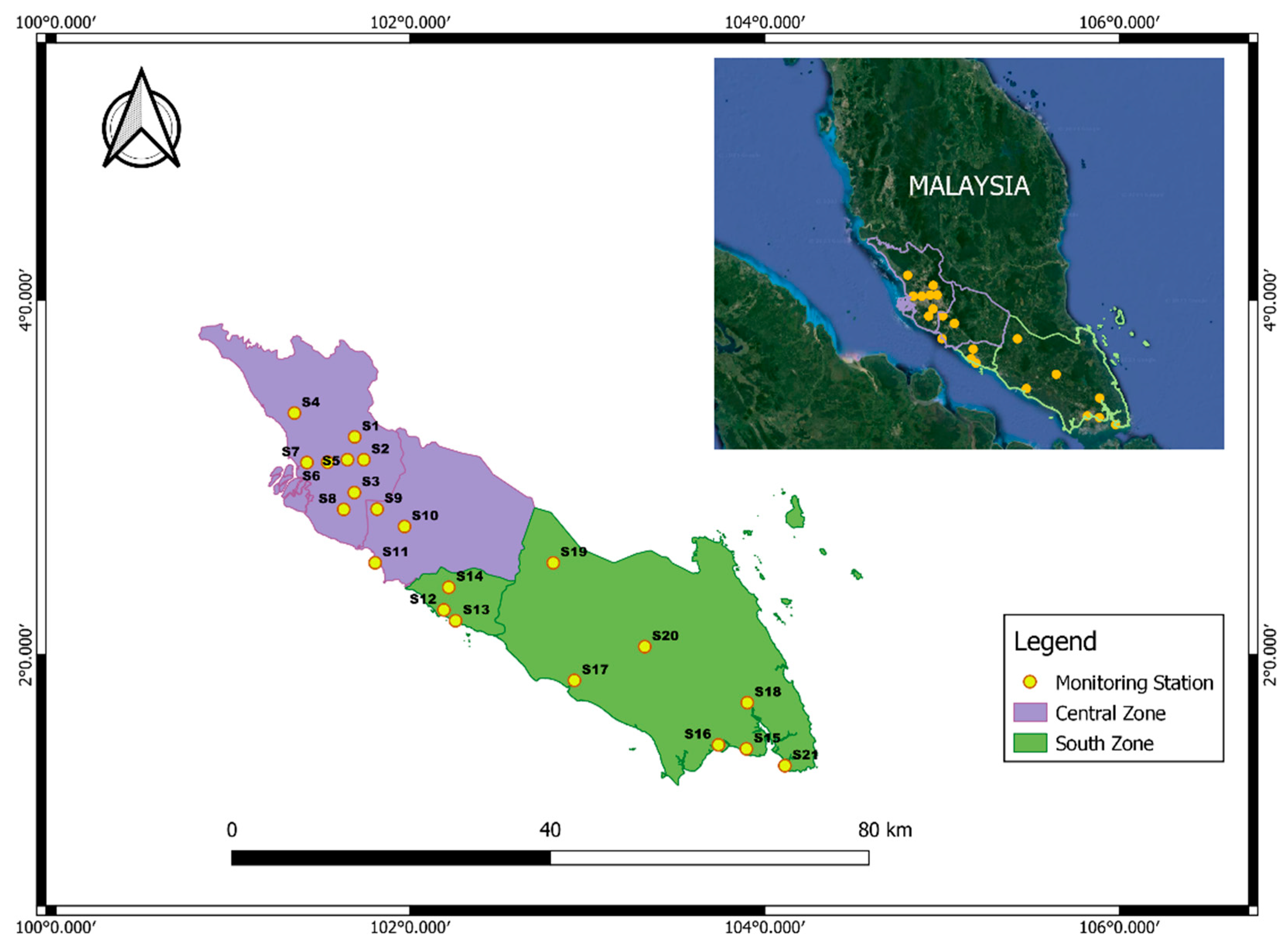
2.1. Study Area

This study focuses on the concentrations of particulate matter with a diameter size below 2.5 μm (PM_2.5). The study area in Peninsular Malaysia has been divided into two zones: the central zone and the south zone (Figure 1).

The central zone, situated in the heart of Peninsular Malaysia, encompasses the states of Selangor, Kuala Lumpur, Putrajaya, and Negeri Sembilan. This region is commonly referred to as the Kuala Lumpur mega-metropolitan environment and encompasses the Klang Valley. The Klang Valley region is widely recognized as the most developed area in Malaysia, boasting the highest population in the country. Kuala Lumpur functions as the capital city of Malaysia and holds the status of a federal territory. This region, which encompasses Putrajaya, functions as the administrative capital of Malaysia. The central zones are predominantly characterized as urban and semi-urban environments, primarily due to population expansion, increased industrial and economic activity, and their role as the administrative center for the federal government. The central zone is additionally impacted by industrial activity and transportation emissions resulting from a significant concentration of motor vehicles, particularly within Kuala Lumpur city center.

The south zone consists of two states, Melaka and Johor. This area is dominated by urban and industrial activities, especially in the southern region of Johor and next to Singapore. Most of the urban environments and townships are located on the west coast, and the rural area is located toward the middle of the peninsula. Cities such as Melaka Tow and Johor Bahru are usually influenced by heavy traffic and industrial activities. As well as by local emissions, the air quality in the central and south zones is influenced by transboundary emissions, especially from Sumatra Indonesia during the southwest monsoon.

The average annual temperature for Peninsular Malaysia is about 26 °C, with little variation between months. Both zones have two distinct seasons: the northeast monsoon (November to March) and the southwest monsoon (May to September). The northeast monsoon brings heavy rainfall and thunderstorms to the zone, while the southwest monsoon brings drier and cooler air. The average annual rainfall is about 2000 mm, with most of it falling during the northeast monsoon.

2.2. Data Collection and Analysis

The concentrations of PM_2.5 were collected at 11 continuous air quality monitoring stations (CAQMSs) in the central zone and 10 CAQMSs in the south zone of Peninsular Malaysia. Table S1 (Supplementary Material) shows the description of the monitoring stations in Kuala Lumpur, Putrajaya, Selangor, Negeri Sembilan (central zone), and Melaka and Johor (south zone) as additional information. Figure 1 shows the location of each monitoring station in the central and south zones of Peninsular Malaysia. All the CAQMS are operated by Pakar Scieno TW Sdn Bhd on behalf of the Malaysian Department of Environment. A Thermo Scientific tapered element oscillating microbalance (TEOM) 1405-DF (USA) was used to determine PM_2.5 concentrations. All calibration procedures and quality control/quality assurance (QA/QC) of the data were conducted via Pakar Scieno TW Sdn Bhd (Shah Alam, Malaysia) before the data were submitted to the Malaysian Department of Environment [27,28]. In this study, data analysis has been conducted using the library “geoR” and the “gstat” package in R version 4.1.2, SAGA GIS 7.8.2, and QGIS version 3.26.2 software produced the raster image and mapping of the study area.

2.3. Classification Breakpoint of PM_2.5 Concentrations in the Air Pollutant Index (API)

The breakpoint of PM_2.5 for API calculation is based on the concentration suggested by the Malaysian Department of Environment, which, in turn, is based on the breakpoint concentrations adopted by the United States Environmental Protection Agency (US EPA). There are a few categories of breakpoints of PM_2.5 concentrations for 24 h averages that will be referred to in this study: Good (0–12.0 µg/m³); Moderate (12.1–35.4 µg/m³); Unhealthy for Sensitive Groups (35.5–55.4 µg/m³); Unhealthy (55.5–150.4 µg/m³); and Very Unhealthy (150.5–250.4 µg/m³), based on the United States Environment Protection Agency (USEPA) recommendations [29]. Based on the Malaysian Ambient Air Quality Standard, the standard 24 h average particulate matter with sizes of less than 2.5 microns (PM_2.5) is 35 µg/m³, whereas for one year, it is 15 µg/m³.

2.4. Spatial Autocorrelation

In this study, PM_2.5 concentration is the main parameter to be evaluated based on data from different stations. The spatial autocorrelation (Moran’s I) was used to calculate the spatial autocorrelation based on the location and value of the parameter.

2.4.1. Moran’s I Method

Patrick Alfred Pierce Moran created the Moran’s I scale to measure spatial autocorrelation. A correlation in a signal between close-by spatial locations essentially defines spatial autocorrelation. Moran’s I is written as (1):

$$I=\frac{N}{{\sum }_I{\sum }_j{\mathcal{w}}_{ij}}\frac{{\sum }_I{\sum }_j{\mathcal{w}}_{ij}({\mathcal{x}}_i-\overline{\mathcal{x}})({\mathcal{x}}_j-\overline{\mathcal{x}})}{{\sum }_i{({\mathcal{x}}_i-\overline{\mathcal{x}})}^2}$$

(1)

where N is the quantity of spatial units that are indexed by both I and j, $x$ is the variable of interest, $\overline{\mathcal{x}}$ is the mean of $x$, and ${\mathcal{w}}_{ij}$ is a spatial weights matrix where the diagonal contains zero (i.e., ${\mathcal{w}}_{ii}=0)$.

Moran’s I employs the subsequent null and alternative hypotheses:

H₀. 

The data are randomly dispersed.

H_A. 

The data are not randomly dispersed (they are clustered in noticeable patterns).

The $z_I$-score for the statistics is calculated as

$$z_I=\frac{I-E\left[I\right]}{\sqrt{V\left[I\right]}}$$

(2)

where $E\left[I\right]$ and $V\left[I^2\right]$ are

$$E\left[I\right]=-1/(n-1)$$

(3)

$$V\left[I^2\right]=E\left[I^2\right]-{E\left[I\right]}^2$$

(4)

where $E\left[I\right]$ is the predicted index value, and $V\left[I^2\right]$ is the index value of variance.

The method uses hypothesis testing to determine whether the specified pattern is clustered, scattered, or random, given a set of associated features and attributes. To assess the significance of Moran’s I index, the tool calculates its value along with the $z_I$-score and p-value. If the p-value for Moran’s I is less than a specified level of significance (i.e., a = 0.05), and the $z_I$-score is positive, then the null hypothesis is rejected. The dataset exhibits a more spatially concentrated distribution of high and/or low values than one could anticipate from random underlying spatial processes. If the p-value for Moran’s I is less than a specified level of significance (i.e., a = 0.05), and the $z_I$-score is negative, then we may reject the null hypothesis. The dataset’s spatial distribution of high and low values is more dispersed than expected if the underlying spatial processes were random [30,31].

2.4.2. Variogram

The variogram is an important input in kriging interpolation. In order to describe the geographical variation in the pollutant concentrations, the geostatistical procedure known as kriging defines a correlation (semi-variogram) among the sample locations [32]. This is a statistical measure that quantifies the spatial correlation between two points. An exploratory data analysis tool that plots half of the mean squared difference between paired observations against their separation distance is called an experimental variogram. The variogram shows how comparable the values are between close measurements. The experimental variogram can be fitted with a variogram model. For kriging, the model coefficients are necessary [33]. The variogram is the random process Z(x), a theoretical function that, we believe, is responsible for the actual realization on the ground [34]. The spatial variability of the regional variables between two places is characterized using the variogram. Equation (5) is utilized to calculate data pairs that are separated by the distance h using the semi-variogram γ(h);

$$\gamma \left(h\right)=\frac{1}{2N\left(h\right)}\left\{{\sum }_{i=1}^{N\left(h\right)}{[Z\left(x_i+h\right)-Z\left(x_i\right)]}^2\right\}$$

(5)

where h denotes the lag distance between two observation locations, Z ($x_i$) is the value of the regional variable of interest at the observation at the observation locations $x_i$, Z ($x_i+h$) is the regional variable of interest value at the specified location $x_i+h$, and N(h) is the quantity of data pairs at the observation locations divided by h. h is represented by a distance interval, since there is little chance that the distance between the sampled pairs will be accurate.

A fitted semi-variogram contains the three components of nugget, range, and sill. The sill, which is made up of the nugget and the partial sill, is the height at which the semi-variogram levelling is removed. The range is the distance from the sill at which the semi-variogram levelling occurs. The measurement errors or micro-scale differences are represented by the nugget effect [23]. The semi-variogram model, the quantity N of PM_2.5, and its spatial position all affect the predicted variance. Consequently, selecting the right semi-variogram model is crucial for determining the best estimation variance. The semi-variogram obtained from the experimental data at the observation site is compared to a theoretical semi-variogram model of γ(h). Exponential, Gaussian, and stable semi-variogram models were written as selected to fit a model [35]:

• Exponential model

$$\gamma \left(h\right)=b+c_0(1-e^{-\frac{h}{a}})$$

(6)

$$a \mathrm{i}\mathrm{s} \mathrm{t}\mathrm{h}\mathrm{e} \mathrm{r}\mathrm{a}\mathrm{n}\mathrm{g}\mathrm{e} \mathrm{p}\mathrm{a}\mathrm{r}\mathrm{a}\mathrm{m}\mathrm{e}\mathrm{t}\mathrm{e}\mathrm{r} \mathrm{t}\mathrm{h}\mathrm{a}\mathrm{t} \mathrm{c}\mathrm{a}\mathrm{n} \mathrm{b}\mathrm{e} \mathrm{c}\mathrm{a}\mathrm{l}\mathrm{c}\mathrm{u}\mathrm{l}\mathrm{a}\mathrm{t}\mathrm{e}\mathrm{d} \mathrm{f}\mathrm{r}\mathrm{o}\mathrm{m} \mathrm{t}\mathrm{h}\mathrm{e} \mathrm{e}\mathrm{f}\mathrm{f}\mathrm{e}\mathrm{c}\mathrm{t}\mathrm{i}\mathrm{v}\mathrm{e} \mathrm{r}\mathrm{a}\mathrm{n}\mathrm{g}\mathrm{e}r \mathrm{a}\mathrm{s}:a=\frac{r}{3}$$

where $h$ specifies the lag of separating distances from which the dependent variable shall be calculated. It must be a positive real number, $r$ is the effective range, and the effective range is the lag where 95% of the sill is exceeded. This is necessary because an exponential function can only approach the sill asymptotically. $c_0$ represents the sill of the variogram where it will flatten out; $b$ represents the nugget of the variogram.

• Gaussian model

$$\gamma \left(h\right)=b+c_0(1-e^{-\frac{h^2}{a^2}})$$

(7)

$$a=\frac{r}{2}$$

• Stable model

$$\gamma \left(h\right)=b+C_0\left(1-e^{-{\frac{h}{a}}^s}\right)$$

(8)

$$a=\frac{r}{3^{\frac{1}{s}}}$$

where $h$ specifies the lag of the separating distances that the dependent variable shall be calculated from, and $r$ is the effective range. The latency at which 95% of the sill is exceeded is the effective range. This is necessary since the e-function portion of the stable model only approaches the sill asymptotically. $c_0$ is the sill of the variogram where it will flatten out and is the shape parameter. For s ≤ 2, the model will be shaped more like an exponential or spherical model; for s > 2, it will be shaped most like a Gaussian function. $b$ is the nugget of the variogram.

2.5. Spatial Interpolation

Kriging is a family of interpolation processes in the geostatistical method after IDW (inverse-distance-weighted) and spline interpolation. Kriging is a multi-step procedure that involves investigating a variance surface as well as exploratory statistical analysis of the data, variogram modelling, surface creation, and surface exploration (if applicable). The kriging interpolation technique is the best linear unbiased estimator (BLUE). It represents the spatial autocorrelation of pairs of points in space and creates a minimum variance of the predicted error by analyzing a variogram. When the forms of the semi-variogram are known, it is possible to estimate the concentrations of the variables at any unsampled location using kriging techniques [35]. There are different techniques that apply in this study: ordinary kriging (OK), simple kriging (SK), and universal kriging (UK).

2.5.1. Ordinary Kriging

The basic geostatistical approach for simulating the geographical distribution of a random variable is known as ordinary kriging (OK). The OK method is an optimal spatial interpolation estimation method in which the value of the random variable $Z\left(x\right)$ at an unsampled location $x_0$ is determined according to the linear combination of the known values of all the sampled locations, as follows:

$$Z^{\ast }\left(x_0\right)={\sum }_{i=1}^M{\lambda }_i\left(x_i\right)Z\left(x_i\right)$$

(9)

where $x_i$ is a sample location between Station 1 and Station 21, $x_0$ is the unsampled location, $Z^{\ast }\left(x_0\right)$ is the unknown value of the random variable (PM_2.5) to be determined at the unsampled location $x_0, Z\left(x_i\right)$ denotes the known value of the random variable (PM_2.5) at the sample location $\left(x_i\right)$, M is the total number of known values of the random variable $Z\left(x_i\right)$ at the sampled location, and ${\lambda }_i\left(x_i\right)$ is a kriging weighted factor for the knockdown of the random variable Z(x) at the sampled location $\left(x_i\right)$, which is used to determine $Z^{\ast }\left(x_0\right)$ [36]. ${\lambda }_i\left(x_i\right)$ is the weight that indicates the contribution from observations to ensure that $Z^{\ast }\left(x_0\right)$ is unbiased; the optimized unbiased estimation represents the average of the estimated error, or the residuals close to zero, as a mathematical expectation of the difference between the predicted value $Z^{\ast }\left(x_0\right)$ and the observed value $Z\left(x_i\right)$. The goal is to minimize the variation between the predicted $Z\left({\mu }_0\right)$ and observed value of $Z\left(x_i\right)$ [37]. Ordinary kriging can use either semi-variograms or covariances, transformations and remove trends, and allows measurement error. Fitri et al. [38] explains that ordinary kriging has a good level of accuracy when estimating the concentrations of PM_2.5 in Surabaya.

2.5.2. Simple Kriging

An estimate is created using simple kriging (SK), which modifies the mean. In an SK equation, the stationary random variable’s mean value, $m\left(x\right)$, is presumed to be constant and well known throughout the research zones. The SK estimator must be fair and have a small variance in the estimate error for the global mean assumption to hold true. The SK equation is written as (10):

$$Z^{\ast }\left(x\right)={\sum }_{i=1}^n{\lambda }_i\left(x_i\right)·Z\left(x_i\right)+[1-{\sum }_{j=1}^M{\lambda }_j\left(x_j\right)]m$$

(10)

where $Z^{\ast }\left(x\right)$ is the random variable (PM_2.5) at the location $x$, $x_i$ values are equal to M data locations, $m\left(x\right)=E\left\{Z\left(x\right)\right\}$ is equal to the location-dependent expected values of the random variable $Z^{\ast }\left(x\right)$, $Z^{\ast }\left(x\right)$ is the linear regression estimator, ${\lambda }_i\left(x_i\right)$ is the weight, and $m\left(x\right)$ is the mean [35].

2.5.3. Universal Kriging

Universal kriging (UK) is kriging with a trend and is similar to OK. The UK addresses a situation in which the local mean varies within the research region. Even though the local mean $m\left(x\right)$ is unknown, much like in OK, the UK models are a linear combination of coordinate functions. UK can handle a nonstationary mean in which the predicted value of $Z\left(x\right)$ is a linear or high-order deterministic function of the $\left(x,y\right)$ coordinates of the data points. The random function $Z\left(x\right)$ is a combination of trend components with a deterministic variation, $m\left(x\right)$ and a residual component, $R\left(x\right)$. The UK is described as

$$Z^{\ast }\left(x\right)=m\left(x\right)+R\left(x\right) \mathrm{a}\mathrm{n}\mathrm{d} m\left(x\right)=E\left\{Z\left(x\right)\right\}={\sum }_{i=0}^n{\mu }_i{\lambda }_i\left(x_i\right)$$

(11)

where ${\lambda }_i\left(x\right)$ is the kriging weighted factor, and ${\mu }_i$ is the fixed, unknown coefficient, $Z^{\ast }\left(x\right)$ is the random function, $m\left(x\right)$ is a trend component with a deterministic variation, and $R\left(x\right)$ is a residual component [35].

2.6. Performance Indicator

The spatial variability needed for the kriging approach can be explained using the theoretical semi-variogram model [37]. The mean squared error (MSE), root-mean-square error (RMSE), and normalized root-mean-square error (NRMSE) were used to validate the error of estimates [39]:

$$MSE=\frac{1}{N}{\sum }_{i=1}^N{\left(\right(z\left(x_i\right)-\widehat{z}\left(x_i\right))}^2$$

(12)

$$RMSE=\sqrt{\frac{1}{N}{\sum }_{i=1}^N\left[{(z\left(x_i\right)-\widehat{z}(x_i\left)\right)}^2\right]}$$

(13)

$$NRMSE=\frac{RMSE}{{\max }_{i}z\left(x_i\right)-{min}_{i}z\left(x_i\right)}$$

(14)

where $z\left(x_i\right)$ is the actual value of PM_2.5 at the location i, $\widehat{z}\left(x_i\right)$ is the prediction value at location i, and $N$ is the number of observations.

3. Results

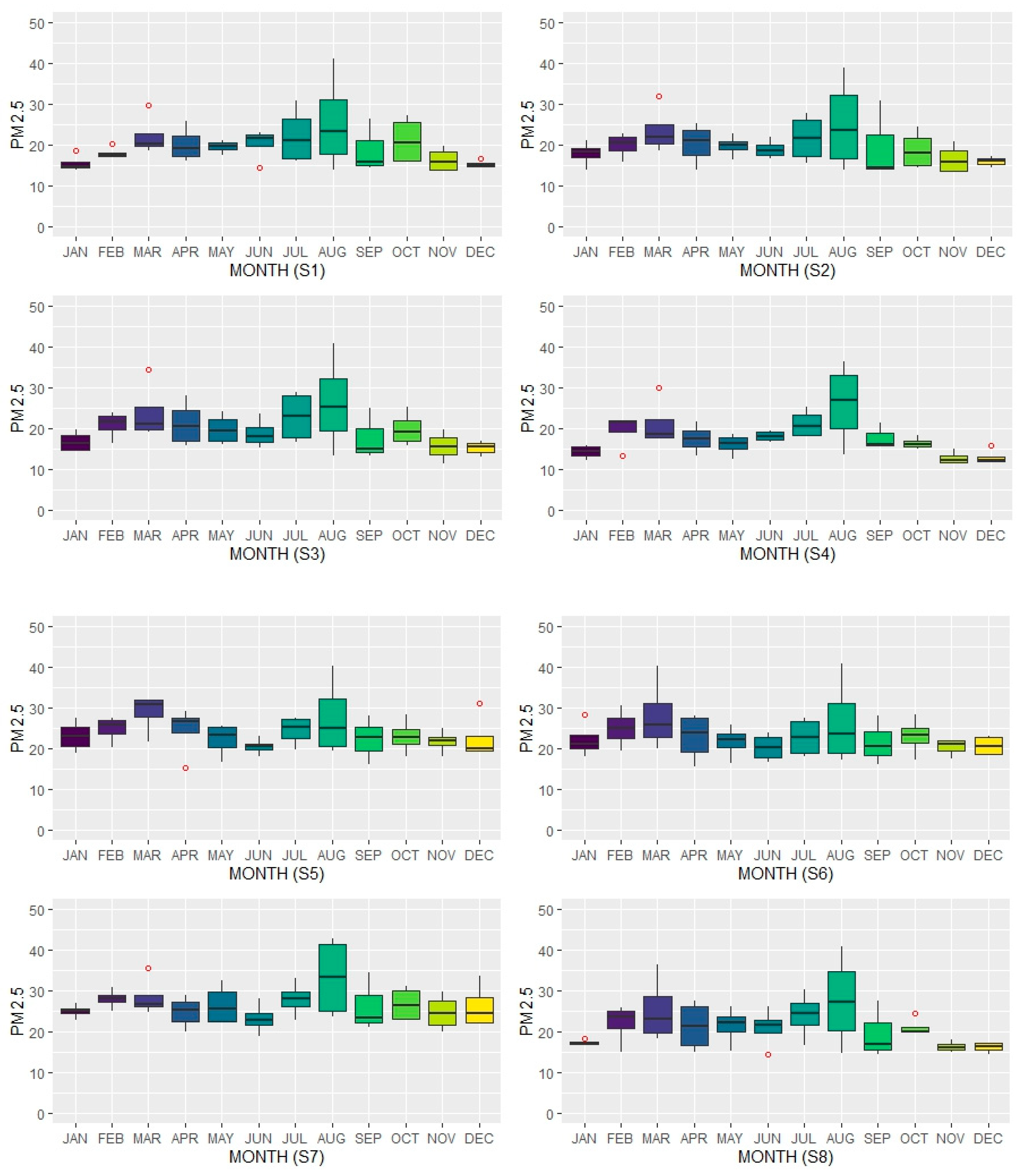
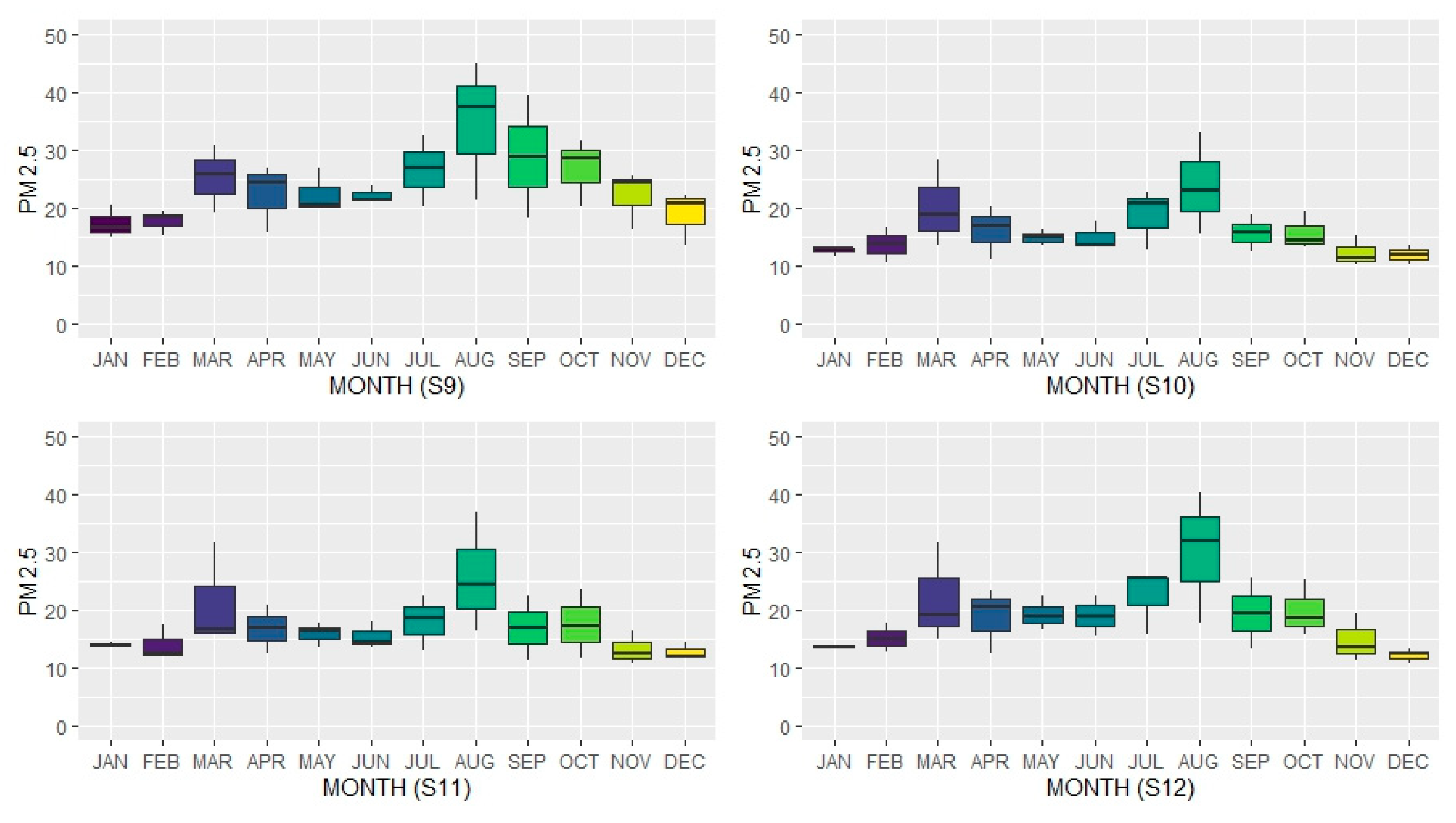
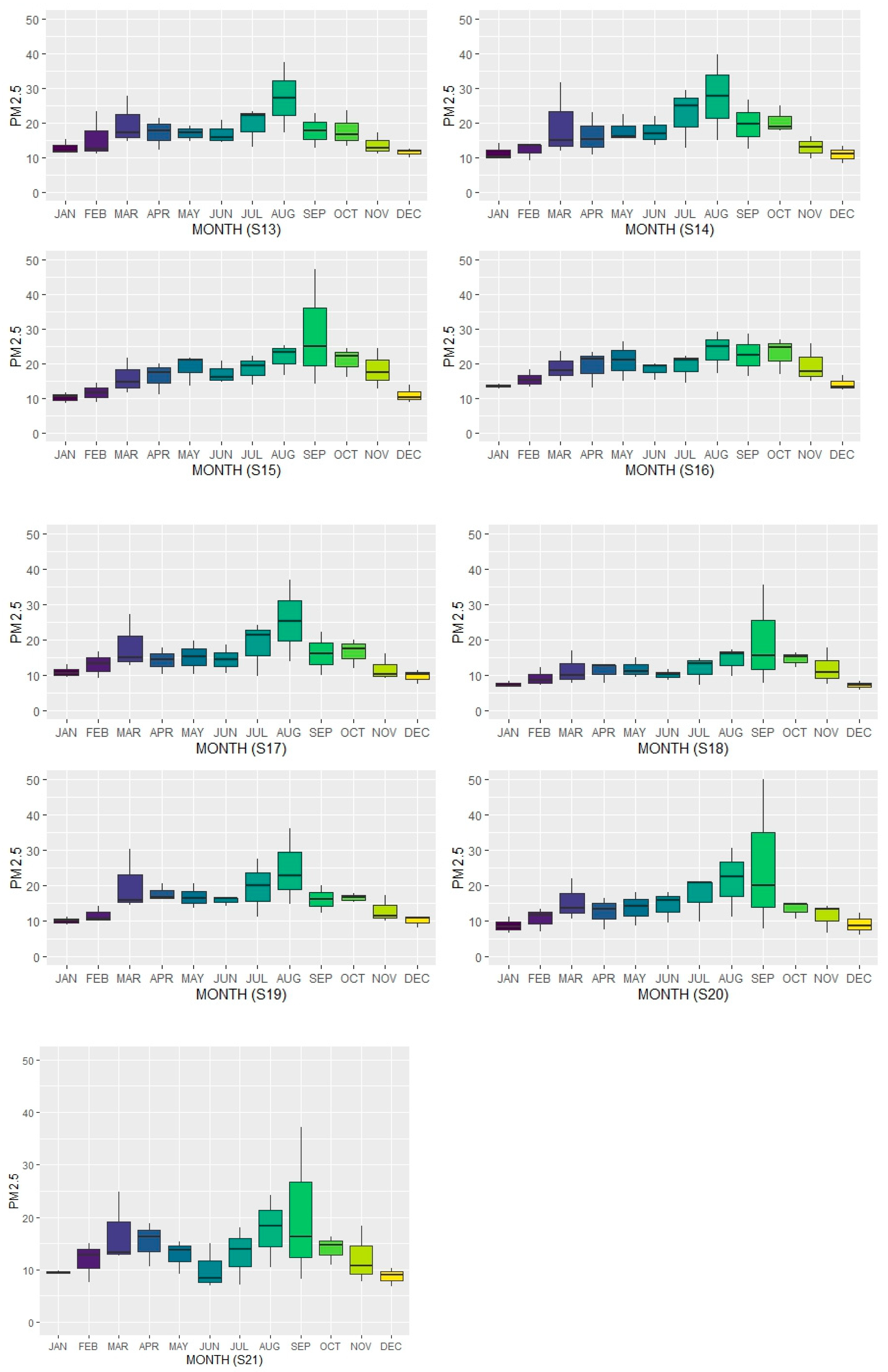
3.1. Descriptive Analysis of PM_2.5 Concentrations

Table 1. Descriptive analysis of annual average PM_2.5 concentration data of twenty-one stations in 2019 and 2020.

Year	2019					2020
Station	Mean	Median	SD	Min	Max	Mean	Median	SD	Min	Max
S1	28.39	23.95	16.90	14.60	76.60	17.50	16.95	2.61	14.00	22.10
S2	28.23	23.00	16.07	16.40	75.00	15.78	15.65	1.70	13.70	18.50
S3	29.79	24.60	16.85	16.20	78.60	16.62	16.25	2.11	14.30	21.30
S4	24.12	19.70	14.83	11.70	65.10	15.23	14.50	3.06	11.70	22.00
S5	30.09	25.80	15.93	19.10	77.10	19.97	19.10	4.37	15.30	31.10
S6	32.18	28.20	15.46	18.80	76.40	18.07	18.05	1.63	15.50	20.70
S7	33.07	30.35	14.34	18.90	74.10	23.23	22.75	1.98	19.90	26.90
S8	29.32	25.15	15.66	14.50	72.60	17.02	16.70	2.22	14.50	22.00
S9	30.14	25.01	18.64	13.68	82.46	18.91	19.50	2.38	15.21	22.30
S10	22.56	17.44	15.33	10.27	66.32	12.67	12.87	1.49	10.18	15.59
S11	24.10	19.33	15.76	11.75	67.66	13.08	12.75	1.70	10.71	16.36
S12	25.92	22.80	14.64	10.95	64.82	14.37	14.28	1.99	11.42	17.79
S13	23.46	20.28	14.36	10.03	62.05	13.21	12.95	1.78	11.20	17.25
S14	25.07	22.79	15.05	8.44	64.49	12.48	12.18	2.67	9.126	17.73
S15	21.06	20.84	9.91	8.87	47.29	12.69	13.21	2.66	8.536	16.54
S16	24.66	23.49	11.46	12.60	56.86	14.78	14.96	1.47	12.80	17.19
S17	22.08	18.80	12.90	7.49	54.97	10.64	10.24	1.51	9.122	14.00
S18	14.82	14.18	7.60	5.92	35.51	8.27	7.789	1.46	6.95	12.07
S19	23.72	19.21	16.40	7.97	68.71	12.96	12.90	2.55	9.92	16.63
S20	19.28	16.07	11.44	6.11	49.49	8.64	8.60	1.53	6.72	11.07
S21	16.94	14.31	8.54	6.89	37.17	9.16	9.13	1.72	6.99	12.67

lists the descriptive information on PM_2.5 concentrations from 2019 to 2020 at twenty-one monitoring stations in Selangor, Kuala Lumpur, Putrajaya, Negeri Sembilan, Melaka, and Johor. According to the Malaysian Ambien Air Quality Standard (MAAQS), in a year, the acceptable level of PM_2.5 is 15 µg/m³. Only S1, S2, S3, S4, S8, S6, S7, S8, and S9 exceeded the year’s PM_2.5 guideline point in 2020. The average mean for 2019 was above the standard of PM_2.5 for all stations except S18. This station is situated in the city’s central zone, which also happens to be a densely populated and economically active sector. When comparing these two years, we can see that 2019 had extremely high PM_2.5 concentrations since the maximum value was between 35.51 µg/m³ and 78.60 µg/m³, which far exceeded the MAAQS’s year guideline point. These extreme concentrations were the result of an Indonesian forest fire in Sumatra that caused a haze episode [40]. There was high variability recorded at Petaling Jaya station (S5), with standard deviations between 4.37 and 15.93 µg/m³, and Nilai station (S9), with standard deviations between 2.38 and 18.64 µg/m³, compared to other stations.

From Figure 2, the monthly data from the boxplots show that there was an increase in PM_2.5 concentrations between June and August or September due to the southwest monsoon, which is the driest time of the year. High temperatures can constitute one of the reasons for increases in the concentration of PM_2.5 in the atmosphere. The northeast monsoon or rainy season occurs from November to March and causes lower temperatures and PM_2.5 concentrations. April to May and October to November are the inter-monsoon seasons where the winds are assumed to be mostly light and variable compared to the northeast monsoon. The lower wind speeds can affect the increase in PM_2.5 concentrations [41]. There was an increase in concentrations in September due to the haze episode that occurred in 2019, which caused air pollution, increasing particulate matter in that month particularly. This episode was caused by the burning of biomass from Sumatra which affects almost all countries in Southeast Asia, including Malaysia, Thailand, and Brunei, and originated from local sources such as vehicles, factories, power plants, and open combustion [42,43].

3.2. Spatial Autocorrelation

The spatial autocorrelations of PM_2.5 concentrations for the two different years were calculated.

Table 2. Descriptive analysis of Moran’s I in the years 2019 and 2020.

	2019	2020
Observed	0.37	−0.06
Expected	−0.05	−0.05
Standard deviation	0.07	0.06
z-score	6.20	−0.16
p-value	5.62 × 10−10	0.87

presents the descriptive analysis of Moran’s I for the years 2019–2020.

From Table 2, Moran’s I test shows that in the year 2019, the observed value is 0.37 and the expected or predicted value is −0.05. The p-value is 5.62 × 10⁻¹⁰, less than the significance level (i.e., <0.05), and the z-score is positive, so we reject the null hypothesis. It is quite possible that the data are not randomly dispersed or they are clustered in noticeable patterns. In 2019, the Moran’s I test showed significant results based on the p-value indicating that the data were not randomly dispersed. This is due to haze episodes in the studied zones, caused by forest fires in Sumatra, Indonesia [40]. In 2020, the p-value is more than 0.05 at 0.87 and the z-score is negative. Hence, the null hypothesis is not rejected, i.e., the underlying spatial processes were random, and the spatial distribution of low values in the dataset would be less spatially distributed. This is due to a movement control order that only allowed a few industrial and transportation operations in certain areas.

Kriging is currently the best interpolation technique since it is unbiased. However, it needs the data to be dependent and correlated. Hence, a semi-variogram is used in this structural analysis. The initial step in performing a spatial interpolation is to find the semi-variogram. Different interpolation approaches and models can produce different interpolation accuracy and results. The best way to solve a similar problem is to thoroughly analyze the unique properties of various interpolation objects. All these models are unable to guarantee that the resultant estimated value corresponds to the actual one, which precisely illustrates the uncertainty of interpolation [22]. Using MSE and RMSE, the performance of the three models is compared to choose the better model.

The error of each semi-variogram was determined, and the three semi-variogram models were evaluated to choose the best-fitting model, as shown in

Table 3. Comparisons of semi-variogram models used to detect the best-fitting model at the central zone.

Year	2019			2020
Model	MSE	RMSE	NRMSE	MSE	RMSE	NRMSE
Exponential	15.1349	3.8903	20.1584	321.8418	17.9400	90.9503
Gaussian	14.7645	3.8425	19.9101	42.2593	6.5007	32.9561
Stable	15.1398	3.9810	20.1616	19.8337	4.4535	22.5780

and

Table 4. Comparison of semi-variogram models used to detect the best-fitting model at the south zone.

Year	2019			2020
Model	MSE	RMSE	NRMSE	MSE	RMSE	NRMSE
Exponential	12.6802	3.5610	31.9423	90.4825	9.5122	146.1614
Gaussian	12.6796	3.5609	31.9416	57.0498	7.5531	116.0586
Stable	12.6811	3.5611	31.9435	8.8766	2.9793	45.7799

. In the year 2019, the Gaussian model gave the lowest value for MSE in the central zone, which was 14.7645; the RMSE value was 3.8425, and the NRMSE value was 19.9101. In the year 2020, the stable model was the best model selected (MSE = 19.8337, RMSE = 4.4535, NRMSE = 22.5780). In the south zone, the stable model was the best model for both years 2019 (MSE= 12.6811, RMSE = 3.5611, NRMSE = 31.9435) and 2020 (MSE = 8.8766, RMSE = 2.9793, NRMSE = 45.7799) as it gave a lower error than the other models. The best model depends on the characteristics of the datasets.

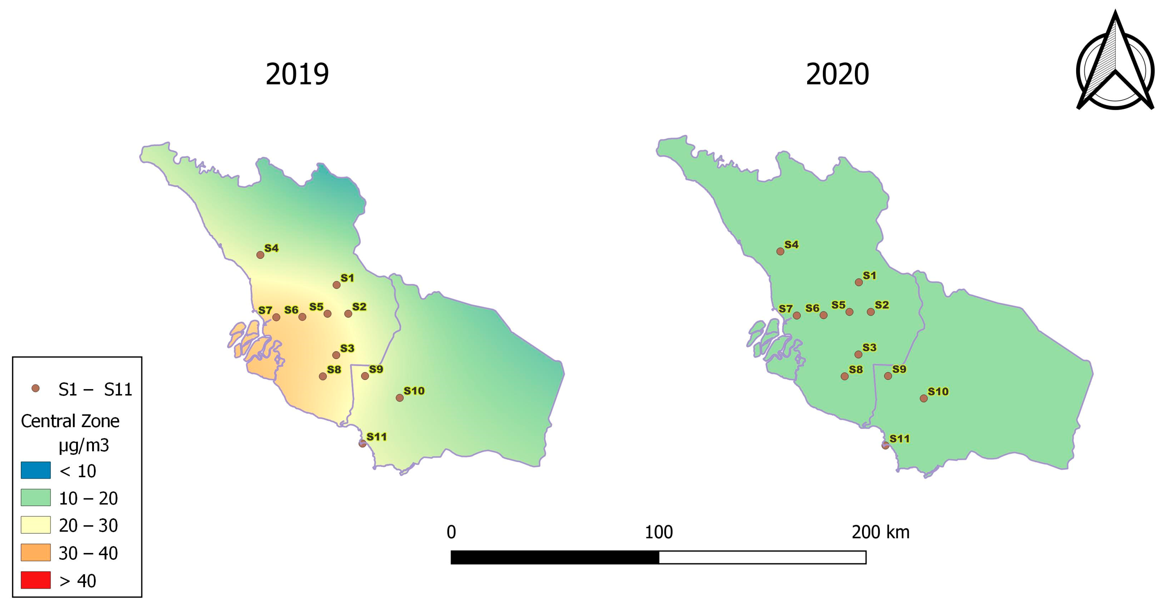
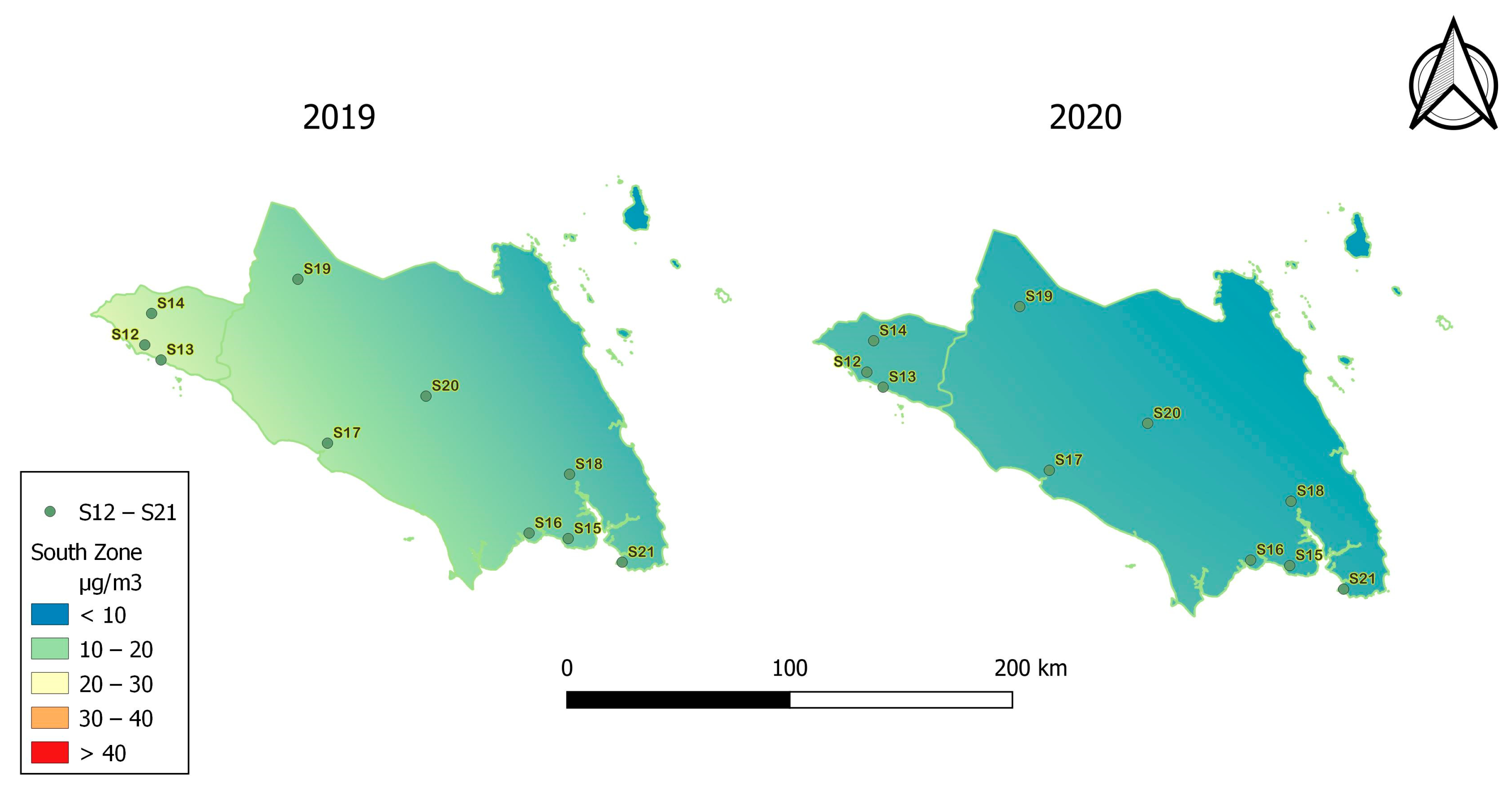
3.3. Temporal Changes in PM_2.5

Using QGIS methods, spatial change maps can be constructed. First, in QGIS, there is SAGA QGIS. Using SAGA QIS, which includes several kriging methods, a raster image is built based on PM_2.5 data via performing interpolation. Next, the raster image is opened in QGIS to find a specific study area for the map produced using the kriging method. Instead, information on a specific can be narrowed down and selected to focus on the study area through looking at a specific color cluster for PM_2.5 in the specific area that cannot be obtained using the data at the monitoring station. From the results of the semi-variogram model, the selected model is used to define the best kriging methods.

1.

Central Zone

Three kriging methods were compared using the performance indicators in the years 2019 and 2020. The results in

Table 5. Cross-validation statistics for PM_2.5 in the central zone.

Year	2019			2020
Method	OK	SK	UK	OK	SK	UK
MSE	19.8333	31.4175	13.9549	15.5617	19.8691	15.1398
RMSE	4.4535	5.6051	3.7356	3.9450	4.4574	3.8909
NRMSE	22.5780	28.4163	18.9385	20.4406	23.0969	20.1616
Ranking	2	3	1 *	2	3	1 *

Note. The best *.

show that the universal kriging method performed better than the other methods for this study, with error values of 13.9549 (MSE), 3.7356 (RMSE), and 18.9385 (NRMSE) for the year 2019. For the year 2020, the universal kriging also showed a better performance, with error values of 15.1398 (MSE), 3.8909 (RMSE), and 20.1616 (NRMS). The central zone, as shown in Figure 3, has 11 stations in Kuala Lumpur, Putrajaya, Selangor, and Negeri Sembilan. At the central zone, there are high concentrations of PM_2.5, shown in the below map with a yellow or orange color (20–40 µg/m³), while the PM_2.5 concentrations are lower in the upper map, with a green color (between 10 and 20 µg/m³). The differences in colors in certain areas due to the emission of PM_2.5 depend on the area classification given in Table S1: urban, suburban, industrial due to industrial activity, or transportation. The differences in color between 2019 and 2020, and the PM_2.5 concentrations in 2019, can be compared to 2020 based on the colors in Figure 3.

2.

South Zone

Table 6. Cross-validation statistics for PM_2.5 in the south zone.

Year	2019			2020
Method	OK	SK	UK	OK	SK	UK
MSE	14.7124	22.4445	12.6811	8.8766	7.8602	5.7940
RMSE	3.8357	4.7375	3.5610	2.9793	2.8036	2.4070
NRMSE	34.4068	42.4970	31.9435	45.7798	43.0793	36.9861
Ranking	2	3	1 *	2	3	1 *

Note. The best *.

explains the cross-validation statistics of three interpolation methods for PM_2.5 in the south zone, which were ordinary kriging, simple kriging, and universal kriging. Based on the performance indicators, universal kriging showed better results when each kriging method was compared. In Table 6, the universal kriging method gives the lowest values for MSE (12.6811), RMSE (3.5610), and NRMSE (31.9435) for the year 2019. In the year 2020, the universal kriging method also performed better, with MSE (5.7940), RMSE (2.4070), and NRMS (36.9861) showing lower errors. The south zone, as shown in Figure 4, has 10 stations in Melaka and Johor. The PM_2.5 concentrations in the south zone are higher in 2019 and are shown as yellow at the bottom of the map (20–30 µg/m³), while lower concentrations of PM_2.5 are shown as green at the top of the map (below 10 µg/m³). Depending on the location’s classification (Table S1)—urban, suburban, industrial due to industrial activities, or transportation—a different color may appear in a given region as a result of PM_2.5 emissions. Figure 4 shows the color difference between 2019 and 2020, as well as the difference in PM_2.5 emission concentrations between 2019 and 2020.

4. Discussion

For spatial autocorrelation, Moran’s I method was used to define the relationship between signals in nearby locations. Then, to define the kriging method, a semi-variogram was needed to define the distance of PM_2.5 concentrations between each location. Through comparing the three models, the best method was selected and used in the kriging method. Comparisons between OK, SK, and UK were carried out to define the better performance based on the data provided. From the map, the central zone (11 stations) showed slightly higher concentrations compared to the south zone. The central zone consists of suburban, urban, and industrial areas with high populations and high economic activities. It shows that the Klang (S7), Shah Alam (S8), and Cheras (S5) monitoring stations had high PM_2.5 concentrations compared to other stations in 2019. The south zone also consists of urban, suburban, and industrial areas.

Figure 3 represents a map of spatiotemporal changes in PM_2.5 concentrations in the central zone using universal kriging. In the year 2019, there was an orange and yellow area on the map because many activities occurred, causing a high mean concentration of PM_2.5. Petaling Jaya (S5), Shah Alam (S6), Klang (S7), and Nilai (S9) are stations located in urban, suburban, and industrial areas with high socioeconomic activities that release PM_2.5. In the year 2020, the concentration of PM_2.5 was less than 10 to 20 µg/m³, in the moderate categories, which was lower compared to the previous year because minimum activity occurred due to the COVID-19 outbreak. Most non-essential activities were required to close to prevent the spread of the virus and to keep people at home. This result indicates that due to the stay-at-home order, the concentrations of PM_2.5 were reduced compared to before the COVID-19 era. Fuel combustion decreased along with the reduction in traffic volume brought on by COVID-19. As a result, the concentrations of smaller particles (PM_2.5) kept dropping. However, not all industries were shut down, including those that dealt with food and those that produced items like masks and sanitizers that were relevant to COVID-19 [44]. The Klang station shows an increased concentration of PM_2.5 to 20–30 µg/m³, but still in the moderate categories. Klang is where Port Klang is located, which is the 12th busiest transshipment port in the world. Despite COVID-19, the port operated normally. Therefore, the contribution of these industries and associated dust still led to a rise in the concentration of particulate matter (PM) [45].

The spatiotemporal changes provide predictive locations that cannot be reached through interpolation. Based on the comparison of several methods, universal kriging provided better performance using the performance indicators. For the map in Figure 3 and Figure 4, the concentrations of PM_2.5 are in the good and moderate ranges in most areas. In 2019, there was a yellow area of 20–30 µg/m³ PM_2.5 and a green area of 10–20 µg/m³ PM_2.5; therefore, the scale is between good and moderate, while, in 2020, all parts were green because the concentrations of PM_2.5 were 10–20 µg/m³, which is between the good and medium categories. The map shows temporal changes between the years 2019 and 2020. In the year 2019, the concentrations of PM_2.5 were more concentrated in certain areas compared to the year 2020. There were socioeconomic activities with heavy transportation, manufacturing, and combustion occurring in the area during that time [46]. In the year 2020, most activities were shut down due to the COVID-19 outbreak causing people to stay at home. The government implemented a movement control order (MCO) to prevent activities that may have caused the spread of the virus. Some activities still occurred, but at a minimum level [47,48,49]. From the map, we can see that the higher concentrations of PM_2.5 are lower compared to the year 2019.

5. Conclusions

Spatial autocorrelation using Moran’s I was used to define the spatial autocorrelation of PM_2.5 concentrations. The results of the study show that the concentrations of PM_2.5 in 2019 are not randomly distributed because economic activities occurred regularly in certain areas, and haze episodes occurred at that time while, in the year 2020, the concentrations are randomly distributed, based on hypothesis testing due to a movement control order that only allowed a few industrial and transportation operations in certain areas during a certain period in the COVID-19 era. The model that performed better in the years 2019 and 2020 was calculated, a performance indicator was used, and the findings showed that different models should be chosen based on different years. In the central zone, the Gaussian model was the best model in 2019 and the stable model in 2020; in the south zone, the stable model gave the best performance indicators in both 2019 and 2020. There were three kriging methods used: simple kriging, ordinary kriging, and universal kriging. Through comparison with the performance indicators, universal kriging showed a better performance compared to the other kriging methods in both years, 2019 (MSE = 13.9549, RMSE = 3.7356, NRMSE = 18.9385) and 2020 (MSE = 15.1398, RMSE = 3.8909, NRMSE = 20.1616).

There is a limitation due to the small number of monitoring stations and limited data, so some interpolation will not be accurate. More monitoring stations would give more data to interpolate across a specific area. In the future, more air quality data could be added, including the metrological data, and more kriging methods could be used to improve the results. The study should also be expanded to the whole of Peninsular Malaysia and other regions.

References

1. Li, X.; Jin, L.; Kan, H. Air Pollution: A Global Problem Needs Local Fixes. Nature 2019, 570, 437–439. [Google Scholar] [CrossRef]
2. Zeng, Y.; Jaffe, D.A.; Qiao, X.; Miao, Y.; Tang, Y. Prediction of Potentially High PM2.5 Concentrations in Chengdu, China. Aerosol Air Qual. Res. 2020, 20, 956–965. [Google Scholar] [CrossRef]
3. Shen, F.; Zhang, L.; Jiang, L.; Tang, M.; Gai, X.; Chen, M.; Ge, X. Temporal Variations of Six Ambient Criteria Air Pollutants from 2015 to 2018, Their Spatial Distributions, Health Risks and Relationships with Socioeconomic Factors During 2018 in China. Environ. Int. 2020, 137, 105556. [Google Scholar] [CrossRef]
4. Tung, N.T.; Pan, C.-H.; Chen, W.-L.; Wang, C.-C.; Liang, C.-W.; Chien, C.-Y.; Chuang, K.-J.; Thao, H.N.X.; Dung, H.B.; Thuy, T.P.C. Associations of PM2.5 with Chronic Obstructive Pulmonary Disease in Shipyard Workers: A Cohort Study. Aerosol Air Qual. Res. 2022, 22, 210272. [Google Scholar] [CrossRef]
5. Fann, N.L.; Nolte, C.G.; Sarofim, M.C.; Martinich, J.; Nassikas, N.J. Associations between Simulated Future Changes in Climate, Air Quality, and Human Health. JAMA Netw. Open 2021, 4, e2032064. [Google Scholar] [CrossRef]
6. Priyankara, S.; Senarathna, M.; Jayaratne, R.; Morawska, L.; Abeysundara, S.; Weerasooriya, R.; Knibbs, L.D.; Dharmage, S.C.; Yasaratne, D.; Bowatte, G. Ambient Pm2. 5 and Pm10 Exposure and Respiratory Disease Hospitalization in Kandy, Sri Lanka. Int. J. Environ. Res. Public Health 2021, 18, 9617. [Google Scholar] [CrossRef]
7. Shihab, A.S. Identification of Air Pollution Sources and Temporal Assessment of Air Quality at a Sector in Mosul City Using Principal Component Analysis. Pol. J. Environ. Stud. 2022, 31, 1–13. [Google Scholar] [CrossRef]
8. Yang, X.; Xiao, D.; Fan, L.; Li, F.; Wang, W.; Bai, H.; Tang, J. Spatiotemporal Estimates of Daily PM2.5 Concentrations Based on 1-Km Resolution Maiac Aod in the Beijing–Tianjin–Hebei, China. Environ. Chall. 2022, 8, 100548. [Google Scholar] [CrossRef]
9. Lei, R.; Nie, D.; Zhang, S.; Yu, W.; Ge, X.; Song, N. Spatial and Temporal Characteristics of Air Pollutants and Their Health Effects in China During 2019–2020. J. Environ. Manag. 2022, 317, 115460. [Google Scholar] [CrossRef]
10. Amil, N.; Latif, M.T.; Khan, M.F.; Mohamad, M. Seasonal Variability of PM2.5 Composition and Sources in the Klang Valley Urban-Industrial Environment. Atmos. Chem. Phys. 2016, 16, 5357–5381. [Google Scholar] [CrossRef]
11. Mazeli, M.I.; Pahrol, M.A.; Shakor, A.S. a. A.; Kanniah, K.D.; Omar, M.A. Cardiovascular, Respiratory and All-Cause (Natural) Health Endpoint Estimation Using a Spatial Approach in Malaysia. Sci. Total Environ. 2023, 874, 162130. [Google Scholar] [CrossRef]
12. Chen, B.; Hong, C.; Pandey, M.R.; Smith, K.R. Indoor Air Pollution in Developing Countries. World Health Stat. Q. 1990, 43, 127–138. [Google Scholar]
13. Huang, Z.; An, X.; Cai, X.; Chen, Y.; Liang, Y.; Hu, S.; Wang, H. The Impact of New Urbanization on PM2.5 Concentration Based on Spatial Spillover Effects: Evidence from 283 Cities in China. Sustain. Cities Soc. 2023, 90, 104386. [Google Scholar] [CrossRef]
14. Qi, G.; Che, J.; Wang, Z. Differential Effects of Urbanization on Air Pollution: Evidences from Six Air Pollutants in Mainland China. Ecol. Indic. 2023, 146, 109924. [Google Scholar] [CrossRef]
15. Xiao, Q.; Geng, G.; Liang, F.; Wang, X.; Lv, Z.; Lei, Y.; Huang, X.; Zhang, Q.; Liu, Y.; He, K. Changes in Spatial Patterns of PM2.5 Pollution in China 2000–2018: Impact of Clean Air Policies. Environ. Int. 2020, 141, 105776. [Google Scholar] [CrossRef]
16. Silva, C.M.C.a.C.; Nascimento, R.C.; Da Silva, Y.J.a.B.; Barbosa, R.S.; Da Silva, Y.J. a B.; Do Nascimento, C.W.A.; Van Straaten, P. Combining Geospatial Analyses to Optimize Quality Reference Values of Rare Earth Elements in Soils. Environ. Monit. Assess. 2020, 192, 1–13. [Google Scholar] [CrossRef]
17. Wang, B.; Wang, B.; Lv, B.; Wang, R. Impact of Motor Vehicle Exhaust on the Air Quality of an Urban City. Aerosol Air Qual. Res. 2022, 22, 220213. [Google Scholar] [CrossRef]
18. Zhang, X.; Han, L.; Wei, H.; Tan, X.; Zhou, W.; Li, W.; Qian, Y. Linking Urbanization and Air Quality Together: A Review and a Perspective on the Future Sustainable Urban Development. J. Clean. Prod. 2022, 346, 130988. [Google Scholar] [CrossRef]
19. Zhang, W.; Wang, C.; Pan, J.; Zhang, L.; Yan, J. Spatial and Temporal Distribution Characteristics of Urban Air Quality Index During Haze Pollution Episodes in China. Arab. J. Geosci. 2022, 15, 1–16. [Google Scholar] [CrossRef]
20. Jiang, C.; He, X.; Le, Y.; Bao, Y.; Liu, B.; Li, X.; Wang, D. Spatiotemporal Patterns and Driving Forces of Air Quality in Jiangsu Province, China, 2014. Fresenius Environ. Bull. 2018, 27, 4076–4083. [Google Scholar]
21. Danek, T.; Weglinska, E.; Zareba, M. The Influence of Meteorological Factors and Terrain on Air Pollution Concentration and Migration: A Geostatistical Case Study from Krakow, Poland. Sci. Rep. 2022, 12, 11050. [Google Scholar] [CrossRef]
22. Tong, Y.; Yu, Y.; Hu, X.; He, L. Performance Analysis of Different Kriging Interpolation Methods Based on Air Quality Index in Wuhan. In Proceedings of the 2015 Sixth International Conference on Intelligent Control and Information Processing (ICICIP), Wuhan, China, 26–28 November 2015; pp. 331–335. [Google Scholar]
23. Aziz, M.K.B.M.; Yusof, F.; Daud, Z.M.; Yusop, Z.; Kasno, M.A. Comparison of Semivariogram Models in Rain Gauge Network Design. MATEMATIKA 2019, 35, 157–170. [Google Scholar] [CrossRef]
24. Gorai, A.K.; Jain, K.G.; Shaw, N.; Tuluri, F.; Tchounwou, P.B. Kriging Analysis for Spatio-Temporal Variations of Ground Level Ozone Concentration. Asian J. Atmos. Environ. 2015, 9, 247–258. [Google Scholar] [CrossRef]
25. Gia Pham, T.; Kappas, M.; Van Huynh, C.; Hoang Khanh Nguyen, L. Application of Ordinary Kriging and Regression Kriging Method for Soil Properties Mapping in Hilly Region of Central Vietnam. ISPRS Int. J. Geo-Inf. 2019, 8, 147. [Google Scholar] [CrossRef]
26. Belkhiri, L.; Tiri, A.; Mouni, L. Spatial Distribution of the Groundwater Quality Using Kriging and Co-Kriging Interpolations. Groundw. Sustain. Dev. 2020, 11, 100473. [Google Scholar] [CrossRef]
27. Mohtar, A.a.A.; Latif, M.T.; Dominick, D.; Ooi, M.C.G.; Azhari, A.; Baharudin, N.H.; Hanif, N.M.; Chung, J.X.; Juneng, L. Spatiotemporal Variations of Particulate Matter and Their Association with Criteria Pollutants and Meteorology in Malaysia. Aerosol Air Qual. Res. 2022, 22, 220124. [Google Scholar] [CrossRef]
28. Rahman, E.A.; Hamzah, F.M.; Latif, M.T.; Dominick, D. Assessment of Pm2. 5 Patterns in Malaysia Using the Clustering Method. Aerosol Air Qual. Res. 2022, 22, 210161. [Google Scholar] [CrossRef]
29. Latif, M.T.; Dominick, D.; Ahamad, F.; Khan, M.F.; Juneng, L.; Hamzah, F.M.; Nadzir, M.S.M. Long Term Assessment of Air Quality from a Background Station on the Malaysian Peninsula. Sci. Total Environ. 2014, 482, 336–348. [Google Scholar] [CrossRef]
30. Li, H.; Calder, C.A.; Cressie, N. Beyond Moran’s I: Testing for Spatial Dependence Based on the Spatial Autoregressive Model. Geogr. Anal. 2007, 39, 357–375. [Google Scholar] [CrossRef]
31. Moran, P.A. Notes on Continuous Stochastic Phenomena. Biometrika 1950, 37, 17–23. [Google Scholar] [CrossRef]
32. Shukla, K.; Kumar, P.; Mann, G.S.; Khare, M. Mapping Spatial Distribution of Particulate Matter Using Kriging and Inverse Distance Weighting at Supersites of Megacity Delhi. Sustain. Cities Soc. 2020, 54, 101997. [Google Scholar] [CrossRef]
33. Robinson, D.; Lloyd, C.D.; Mckinley, J.M. Increasing the Accuracy of Nitrogen Dioxide (NO2) Pollution Mapping Using Geographically Weighted Regression (Gwr) and Geostatistics. Int. J. Appl. Earth Obs. Geoinf. 2013, 21, 374–383. [Google Scholar] [CrossRef]
34. Oliver, M.; Webster, R. A Tutorial Guide to Geostatistics: Computing and Modelling Variograms and Kriging. Catena 2014, 113, 56–69. [Google Scholar] [CrossRef]
35. Oyana, T.J. Spatial Analysis with R: Statistics, Visualization, and Computational Methods; CRC Press: Boca Raton, FL, USA, 2020. [Google Scholar]
36. Liang, C.-P.; Chen, J.-S.; Chien, Y.-C.; Chen, C.-F. Spatial Analysis of the Risk to Human Health from Exposure to Arsenic Contaminated Groundwater: A Kriging Approach. Sci. Total Environ. 2018, 627, 1048–1057. [Google Scholar] [CrossRef]
37. Fan, Z.; Huang, B.; Peng, C.; Lin, J.; Liao, Y. Simulation of Average Monthly Ozone Exposure Concentrations in China: A Temporal and Spatial Estimation Method. Environ. Res. 2021, 199, 111271. [Google Scholar] [CrossRef]
38. Fitri, D.W.; Afifah, N.; Anggarani, S.M.; Chamidah, N. Prediction Concentration of PM2.5 in Surabaya Using Ordinary Kriging Method. AIP Conf. Proc. 2021, 2329, 060030. [Google Scholar]
39. Chang, Y.; Scrimshaw, M.; Emmerson, R.; Lester, J. Geostatistical Analysis of Sampling Uncertainty at the Tollesbury Managed Retreat Site in Blackwater Estuary, Essex, UK: Kriging and Cokriging Approach to Minimise Sampling Density. Sci. Total Environ. 1998, 221, 43–57. [Google Scholar] [CrossRef]
40. Ma’amor, A.; Noor, N.M.; Jafri, I.a.M.; Addiena, N.A.; Saufie, A.Z.U.; Amin, N.A.; Boboc, M.; Deak, G. Spatial and Temporal Variation of Particulate Matter (PM10 and PM2.5) and Its Health Effects During the Haze Event in Malaysia. J. Atmos. Sci. Res. 2023, 6, 26–47. [Google Scholar] [CrossRef]
41. Redzuan, S.N.; Noor, N.M.; Rahim, N.a.a.A.; Jafri, I.a.M.; Baidrulhisham, S.E.; Ul-Saufie, A.Z.; Sandu, A.V.; Vizureanu, P.; Zainol, M.R.R.M.A.; Deák, G. Characteristics of PM10 Level During Haze Events in Malaysia Based on Quantile Regression Method. Atmosphere 2023, 14, 407. [Google Scholar] [CrossRef]
42. Jafri, I.a.M.; Noor, N.M.; Rahim, N.a.a.A.; Ul-Saufie, A.Z.; Hassan, Z.; Deak, G. Spatial and Temporal Analysis of Particulate Matter (PM10) in Urban-Industrial Environment During Episodic Haze Events in Malaysia. Environ. Asia 2023, 16, 111–125. [Google Scholar]
43. Zainal, S.; Zamre, N.M.; Khan, M. Emission Level of Air Pollutants During 2019 Pre-Haze, Haze, and Post-Haze Episodes in Kuala Lumpur and Putrajaya. Malays. J. Chem. Eng. Technol. (MJCET) 2021, 4, 137–154. [Google Scholar] [CrossRef]
44. Berman, J.D.; Ebisu, K. Changes in Us Air Pollution During the COVID-19 Pandemic. Sci. Total Environ. 2020, 739, 139864. [Google Scholar]
45. Khan, S.; Dahu, B.M.; Scott, G.J. A Spatio-Temporal Study of Changes in Air Quality from Pre-Covid Era to Post-COVID Era in Chicago, USA. Aerosol Air Qual. Res. 2022, 22, 220053. [Google Scholar] [CrossRef]
46. Zulkepli, N.F.S.; Noorani, M.S.M.; Razak, F.A.; Ismail, M.; Alias, M.A. Cluster Analysis of Haze Episodes Based on Topological Features. Sustainability 2020, 12, 3985. [Google Scholar]
47. Latif, M.T.; Dominick, D.; Hawari, N.S.S.L.; Mohtar, A.A.A.; Othman, M. The Concentration of Major Air Pollutants During the Movement Control Order Due to the COVID-19 Pandemic in the Klang Valley, Malaysia. Sustain. Cities Soc. 2021, 66, 102660. [Google Scholar]
48. Liu, F.; Wang, M.; Zheng, M. Effects of COVID-19 Lockdown on Global Air Quality and Health. Sci. Total Environ. 2021, 755, 142533. [Google Scholar]
49. Nadzir, M.S.M.; Ooi, M.C.G.; Alhasa, K.M.; Bakar, M.a.A.; Mohtar, A.a.A.; Nor, M.F.F.M.; Latif, M.T.; Abd Hamid, H.H.; Ali, S.H.M.; Ariff, N.M. The Impact of Movement Control Order (Mco) During Pandemic Covid-19 on Local Air Quality in an Urban Area of Klang Valley, Malaysia. Aerosol Air Qual. Res. 2020, 20, 1237–1248. [Google Scholar]
Figure 1. Zones of Peninsular Malaysia in the center and south.
Sustainability 15 16169 g001
Figure 2. Monthly average boxplots of the PM2.5 concentrations at each station in 2019–2020.
Sustainability 15 16169 g002aSustainability 15 16169 g002bSustainability 15 16169 g002c
Figure 3. The spatiotemporal distributions of PM2.5 for the years 2019 and 2020 in the central zone, showing the mapping of the interpolation using the best kriging method, universal kriging.
Sustainability 15 16169 g003
Figure 4. The spatiotemporal distributions of PM2.5 for the years 2019 and 2020 in the south zone, showing the mapping of the interpolation using the best kriging method, universal kriging.
Sustainability 15 16169 g004