
The Ecological Efficiency of Green Materials in Sustainable Urban Planning—A Model for Its Measurement

 , ,
, ,  , , and
Abstract
:1. Introduction
- Ecological: supporting biodiversity and sustaining ecosystem processes;
- Protective: protecting soil in degraded or sensitive areas (riverbanks, embankments, landslide areas, etc.) and mitigating the effects of land degradation and environmental pollution due to anthropogenic activities;
- Hygienic–sanitary: improving the integral health of citizens and promoting recovery during illness [14];
- Social and recreational: supporting recreational and social needs, thereby making the city more comfortable;
- Cultural, educational, and scientific: providing cultural and educational references that promote the harmonious entanglement of people and nature, as well as foster the scientific understanding of the environment;
- Aesthetic–architectural: improving urban landscape structure and scenery.
2. Methodological Background
2.1. Climate Mitigation
2.2. Air Quality Improvement
2.3. Ecological Connectivity Enhancement and Biodiversity Conservation
2.4. Social Benefits
3. Methodology

| Parameter | Description | Characteristic Value | |
|---|---|---|---|
| i | element of vegetation | ||
| N | Number of vegetation elements | ||
| G | Lot area | ||
| Area occupied by i | |||
| Permeable area | |||
| Semipermeable area | |||
| Permeability coefficient | * | ||
| Fraction of G occupied by i | |||
| h | Height of the tallest vegetation layer | ||
| Number of stems | |||
| Average crown diameter | |||
| Clumping factor | [76] | ||
| Volume of linear green elements parallel to w 1 | |||
| Vegetation density | * | ||
| Average distance among green elements 2 | |||
| Vegetation distance from w | |||
| Leaf area index | * | [77,78] | |
| Extinction coefficient for direct radiation | * | [79] | |
| Extinction coefficient for diffuse radiation | * | [80] | |
| Extinction coefficient for rainfall interception | * | [41] | |
| Efficiency of photosynthesis conversion | * | [80] | |
| Particulate interception capability | 3 | [78] | |
| Insulation effect at increasing | *, | ||
| Isolation effect at increasing | *, | ||
| Photosynthetically active radiation | |||
| Drag coefficient | [81] | ||
| Roughness of the underlying surface | , | [81] | |
| k | von Karman constant | [80] | |
| Attenuation factor | [81] |
| Intermediate Goal | Specific Goal | Equation |
|---|---|---|
| Urban Climate (UC) | Permeability | |
| Rainfall interception | ||
| Transpiration | ||
| Air Quality (AQ) | Photosynthesis | |
| Particulate interception | ||
| Biodiversity (B) | Environmental diversity | |
| Ecological connectivity | ||
| Comfort (C) | Shading | |
| Wind attenuation | ||
| Acoustic and visual insulation |
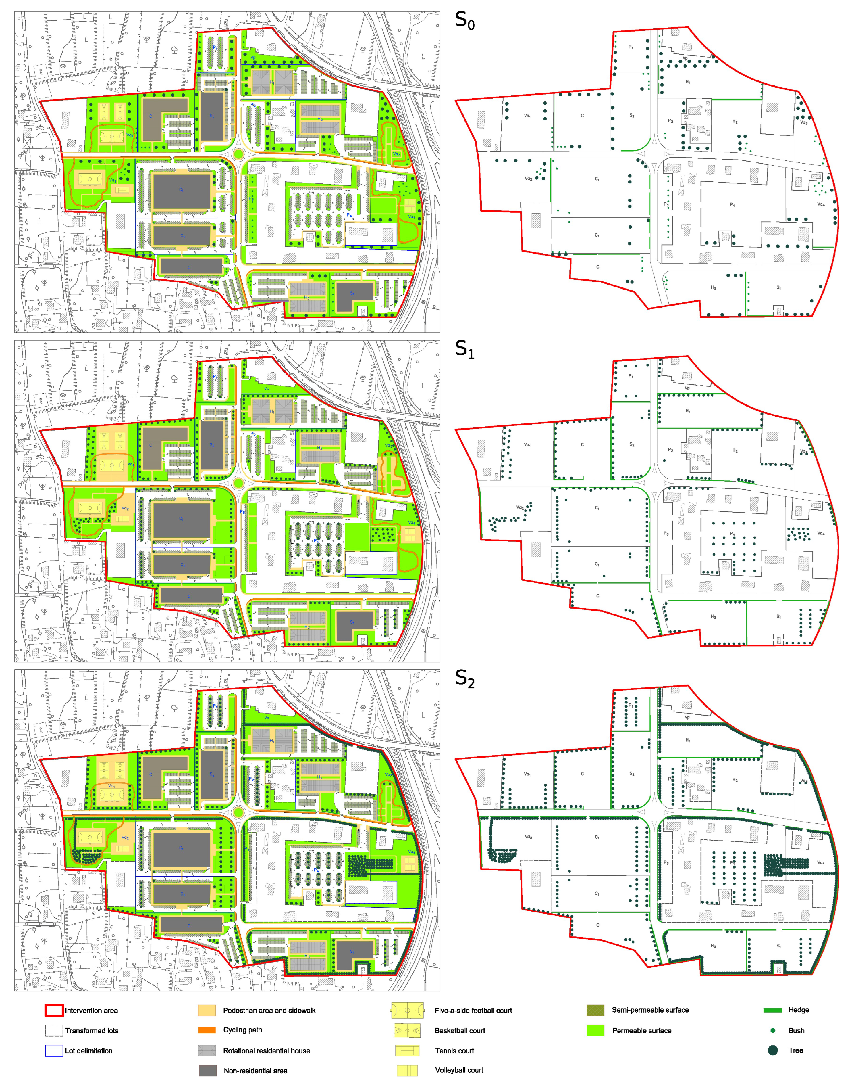
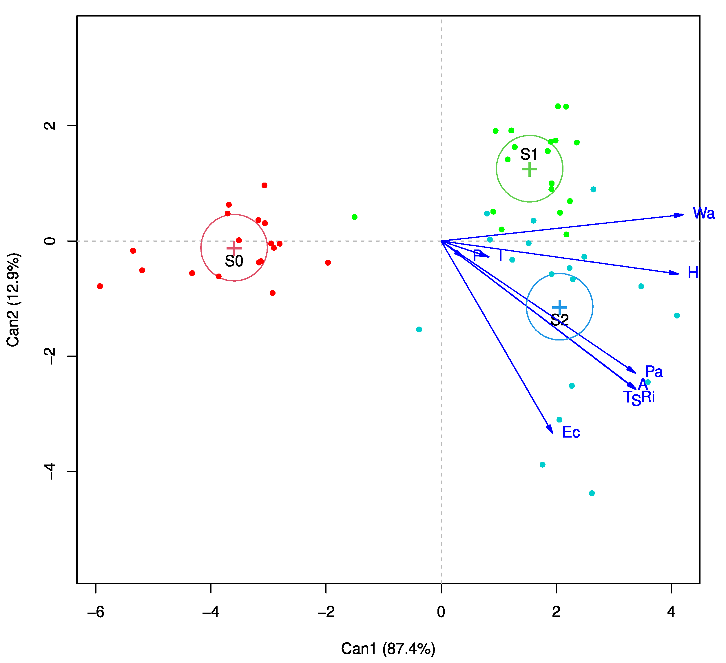
4. Case Study
5. Concluding Remarks
Author Contributions
Funding
Institutional Review Board Statement
Informed Consent Statement
Data Availability Statement
Acknowledgments
Conflicts of Interest
References
- Holling, C.S. Understanding the complexity of economic, ecological, and social systems. Ecosystems 2001, 4, 390–405. [Google Scholar] [CrossRef]
- Grimm, N.B.; Faeth, S.H.; Golubiewski, N.E.; Redman, C.L.; Wu, J.; Bai, X.; Briggs, J.M. Global change and the ecology of cities. Science 2008, 319, 756–760. [Google Scholar] [CrossRef] [PubMed]
- Ostrom, E. A general framework for analyzing sustainability of social-ecological systems. Science 2009, 325, 419–422. [Google Scholar] [CrossRef] [PubMed]
- Geissdoerfer, M.; Savaget, P.; Bocken, N.M.; Hultink, E.J. The circular economy—A new sustainability paradigm? J. Clean. Prod. 2017, 143, 757–768. [Google Scholar] [CrossRef]
- Grădinaru, S.R.; Hersperger, A.M. Green infrastructure in strategic spatial plans: Evidence from European urban regions. Urban For. Urban Green. 2019, 40, 17–28. [Google Scholar] [CrossRef]
- Korkou, M.; Tarigan, A.K.; Hanslin, H.M. The multifunctionality concept in urban green infrastructure planning: A systematic literature review. Urban For. Urban Green. 2023, 85, 127975. [Google Scholar] [CrossRef]
- Honeck, E.; Sanguet, A.; Schlaepfer, M.A.; Wyler, N.; Lehmann, A. Methods for identifying green infrastructure. SN Appl. Sci. 2020, 2, 1–25. [Google Scholar] [CrossRef]
- Pantaloni, M.; Marinelli, G.; Santilocchi, R.; Minelli, A.; Neri, D. Sustainable management practices for urban green spaces to support green infrastructure: An italian case study. Sustainability 2022, 14, 4243. [Google Scholar] [CrossRef]
- Wells, N.M.; Evans, G.W. Nearby nature: A buffer of life stress among rural children. Environ. Behav. 2003, 35, 311–330. [Google Scholar] [CrossRef]
- Dierna, S.; Orlandi, F. Buone Pratiche Per il Quartiere Ecologico; Alinea Editrice: Firenze, Italy, 2005. [Google Scholar]
- Buccolieri, R.; Gromke, C.; Di Sabatino, S.; Ruck, B. Aerodynamic effects of trees on pollutant concentration in street canyons. Sci. Total Environ. 2009, 407, 5247–5256. [Google Scholar] [CrossRef]
- Lindborg, R.; Helm, A.; Bommarco, R.; Heikkinen, R.K.; Kühn, I.; Pykälä, J.; Pärtel, M. Effect of habitat area and isolation on plant trait distribution in European forests and grasslands. Ecography 2012, 35, 356–363. [Google Scholar] [CrossRef]
- Bovo, G.; Miglietta, P.; Peano, O.; Vanzo, A. Manuale Per Tecnici del Verde Urbano; Città di Torino: Torino, Italy, 1998. [Google Scholar]
- Kaplan, R. The nature of the view from home: Psychological benefits. Environ. Behav. 2001, 33, 507–542. [Google Scholar] [CrossRef]
- Kapoor, R.K.; Gupta, V. A pollution attenuation coefficient concept for optimization of green belt. Atmos. Environ. 1984, 18, 1107–1113. [Google Scholar] [CrossRef]
- Kapoor, R.K.; Gupta, V. Attenuation of Air Pollution by Greenbelt; PHI Press: New York, NY, USA, 1992. [Google Scholar]
- Burkhard, B.; Kroll, F.; Müller, F.; Windhorst, W. Landscapes’ capacities to provide ecosystem services—A concept for land-cover based assessments. Landsc. Online 2009, 15, 1–22. [Google Scholar] [CrossRef]
- Burkhard, B.; Kroll, F.; Nedkov, S.; Müller, F. Mapping ecosystem service supply, demand and budgets. Ecol. Indic. 2012, 21, 17–29. [Google Scholar] [CrossRef]
- Fasolino, I.; Grimaldi, M.; Coppola, F. A model for urban planning control of the settlement efficiency: A case study. Arch. Studi Urbani Reg. 2020, 127, 181–210. [Google Scholar] [CrossRef]
- Fasolino, I.; Coppola, F.; Grimaldi, M. Il verde nell’organizzazione urbanistica efficiente degli insediamenti. Una proposta metodologica. In XXII Conferenza Nazionale SIU. L’Urbanistica Italiana di fronte all’Agenda 2030. Portare Territori e Comunità Sulla Strada Della Sostenibilità e Della Resilienza, 5-6-7 Giugno 2019; Planum Publisher: Matera-Bari, Italy, 2020; pp. 1870–1874. [Google Scholar]
- Sanesi, G.; Lafortezza, R. Verde urbano e sostenibilità: Identificazione di un modello e di un set di indicatori. Genio-Rural.-Estimo Territ. 2002, 9, 3–11. [Google Scholar]
- Georgi, N.J.; Zafiriadis, K. The impact of park trees on microclimate in urban areas. Urban Ecosyst. 2006, 9, 195–209. [Google Scholar] [CrossRef]
- Escobedo, F.J.; Kroeger, T.; Wagner, J.E. Urban forests and pollution mitigation: Analyzing ecosystem services and disservices. Environ. Pollut. 2011, 159, 2078–2087. [Google Scholar] [CrossRef]
- Gupta, K.; Kumar, P.; Pathan, S.K.; Sharma, K.P. Urban Neighborhood Green Index—A measure of green spaces in urban areas. Landsc. Urban Plan. 2012, 105, 325–335. [Google Scholar] [CrossRef]
- Toccolini, A. Piano e Progetto di Area Verde. Manuale di Progettazione; Maggioli Editore: Rimini, Italy, 2015. [Google Scholar]
- Dolores, L.; Macchiaroli, M.; De Mare, G. Financial impacts of the energy transition in housing. Sustainability 2022, 14, 4876. [Google Scholar] [CrossRef]
- Rao, P.S.; Gavane, A.; Ankam, S.; Ansari, M.; Pandit, V.; Nema, P. Performance evaluation of a green belt in a petroleum refinery: A case study. Ecol. Eng. 2004, 23, 77–84. [Google Scholar] [CrossRef]
- Nasir, R.A.; Ahmad, S.S.; Zain-Ahmed, A.; Ibrahim, N. Adapting human comfort in an urban area: The role of tree shades towards urban regeneration. Procedia-Soc. Behav. Sci. 2015, 170, 369–380. [Google Scholar] [CrossRef]
- Hsieh, C.M.; Jan, F.C.; Zhang, L. A simplified assessment of how tree allocation, wind environment, and shading affect human comfort. Urban For. Urban Green. 2016, 18, 126–137. [Google Scholar] [CrossRef]
- Hüse, B.; Szabó, S.; Deák, B.; Tóthmérész, B. Mapping an ecological network of green habitat patches and their role in maintaining urban biodiversity in and around Debrecen city (Eastern Hungary). Land Use Policy 2016, 57, 574–581. [Google Scholar] [CrossRef]
- Takács, Á.; Kiss, M.; Hof, A.; Tanács, E.; Gulyás, Á.; Kántor, N. Microclimate modification by urban shade trees—An integrated approach to aid ecosystem service based decision-making. Procedia Environ. Sci. 2016, 32, 97–109. [Google Scholar] [CrossRef]
- Cheela, V.S.; John, M.; Biswas, W.; Sarker, P. Combating urban heat island effect — A review of reflective pavements and tree shading strategies. Buildings 2021, 11, 93. [Google Scholar] [CrossRef]
- Yoshida, S. Effect of growth and types of trees on leaf area density and optical depth on tree canopy. Study on method to evaluate the shading effect of street tree on solar radiation based on field observation. J. Environ. Eng. 2006, 605, 103–110. [Google Scholar] [CrossRef]
- Sasaki, K.; Mochida, A.; Yoshino, H.; Watanabe, H.; Yoshida, T. A new method to select appropriate countermeasures against heat-island effects according to the regional characteristics of heat balance mechanism. J. Wind. Eng. Ind. Aerodyn. 2008, 96, 1629–1639. [Google Scholar] [CrossRef]
- Oke, T.R. Canyon geometry and the nocturnal urban heat island: Comparison of scale model and field observations. J. Climatol. 1981, 1, 237–254. [Google Scholar] [CrossRef]
- Oke, T.; Johnson, G.; Steyn, D.; Watson, I. Simulation of surface urban heat islands under `ideal’ conditions at night part 2: Diagnosis of causation. Bound.-Layer Meteorol. 1991, 56, 339–358. [Google Scholar] [CrossRef]
- Hesslerová, P.; Pokorný, J.; Huryna, H.; Seják, J.; Jirka, V. The impacts of greenery on urban climate and the options for use of thermal data in urban areas. Prog. Plan. 2022, 159, 100545. [Google Scholar] [CrossRef]
- Liu, X.; Li, X.X.; Harshan, S.; Roth, M.; Velasco, E. Evaluation of an urban canopy model in a tropical city: The role of tree evapotranspiration. Environ. Res. Lett. 2017, 12, 094008. [Google Scholar] [CrossRef]
- Xiao, Q.; McPherson, E.G. Rainfall interception by Santa Monica’s municipal urban forest. Urban Ecosyst. 2002, 6, 291–302. [Google Scholar] [CrossRef]
- Asadian, Y.; Weiler, M. A new approach in measuring rainfall interception by urban trees in coastal British Columbia. Water Qual. Res. J. 2009, 44, 16–25. [Google Scholar] [CrossRef]
- Huang, J.Y.; Black, T.; Jassal, R.; Lavkulich, L.L. Modelling rainfall interception by urban trees. Can. Water Resour. J. 2017, 42, 336–348. [Google Scholar] [CrossRef]
- Yang, B.; Lee, D.K.; Heo, H.K.; Biging, G. The effects of tree characteristics on rainfall interception in urban areas. Landsc. Ecol. Eng. 2019, 15, 289–296. [Google Scholar] [CrossRef]
- Kozlowski, T.T. Growth and Development of Trees: Cambial Growth, Root Growth, and Reproductive Growth; Academic Press: New York, NY, USA, 1971. [Google Scholar]
- Day, S.D.; Wiseman, P.E.; Dickinson, S.B.; Harris, J.R. Contemporary concepts of root system architecture of urban trees. Arboric. Urban For. 2010, 36, 149–159. [Google Scholar] [CrossRef]
- Sharma, H.K.; Sharma, M.V.; Janshirani, R.; Gautam, M. Atmospheric carbon control and oxygen production by urban green campus. Res. Rev. J. Life Sci. 2019, 9, 131–139. [Google Scholar]
- Biswal, B.K.; Bolan, N.; Zhu, Y.G.; Balasubramanian, R. Nature-based Systems (NbS) for mitigation of stormwater and air pollution in urban areas: A review. Resour. Conserv. Recycl. 2022, 186, 106578. [Google Scholar] [CrossRef]
- Chaulya, S.; Chakraborty, M.; Singh, R. Air pollution modelling for a proposed limestone quarry. Water Air Soil Pollut. 2001, 126, 171–191. [Google Scholar] [CrossRef]
- Gromke, C.; Ruck, B. Influence of trees on the dispersion of pollutants in an urban street canyon—experimental investigation of the flow and concentration field. Atmos. Environ. 2007, 41, 3287–3302. [Google Scholar] [CrossRef]
- Gromke, C.; Ruck, B. On the impact of trees on dispersion processes of traffic emissions in street canyons. Bound.-Layer Meteorol. 2009, 131, 19–34. [Google Scholar] [CrossRef]
- Gromke, C.; Buccolieri, R.; Di Sabatino, S.; Ruck, B. Dispersion study in a street canyon with tree planting by means of wind tunnel and numerical investigations—Evaluation of CFD data with experimental data. Atmos. Environ. 2008, 42, 8640–8650. [Google Scholar] [CrossRef]
- Gromke, C. A vegetation modeling concept for building and environmental aerodynamics wind tunnel tests and its application in pollutant dispersion studies. Environ. Pollut. 2011, 159, 2094–2099. [Google Scholar] [CrossRef] [PubMed]
- Islam, M.N.; Rahman, K.S.; Bahar, M.M.; Habib, M.A.; Ando, K.; Hattori, N. Pollution attenuation by roadside greenbelt in and around urban areas. Urban For. Urban Green. 2012, 11, 460–464. [Google Scholar] [CrossRef]
- De Nicola, F.; Murena, F.; Costagliola, M.A.; Alfani, A.; Baldantoni, D.; Prati, M.V.; Sessa, L.; Spagnuolo, V.; Giordano, S. A multi-approach monitoring of particulate matter, metals and PAHs in an urban street canyon. Environ. Sci. Pollut. Res. 2013, 20, 4969–4979. [Google Scholar] [CrossRef]
- Li, J.F.; Zhan, J.M.; Li, Y.S.; Wai, O.W. CO2 absorption/emission and aerodynamic effects of trees on the concentrations in a street canyon in Guangzhou, China. Environ. Pollut. 2013, 177, 4–12. [Google Scholar] [CrossRef]
- Lingua, G.; Todeschini, V.; Grimaldi, M.; Baldantoni, D.; Proto, A.; Cicatelli, A.; Biondi, S.; Torrigiani, P.; Castiglione, S. Polyaspartate, a biodegradable chelant that improves the phytoremediation potential of poplar in a highly metal-contaminated agricultural soil. J. Environ. Manag. 2014, 132, 9–15. [Google Scholar] [CrossRef]
- Maisto, G.; Baldantoni, D.; De Marco, A.; Alfani, A.; Virzo De Santo, A. Ranges of nutrient concentrations in Quercus ilex leaves at natural and urban sites. J. Plant Nutr. Soil Sci. 2013, 176, 801–808. [Google Scholar] [CrossRef]
- De Nicola, F.; Baldantoni, D.; Maisto, G.; Alfani, A. Heavy metal and polycyclic aromatic hydrocarbon concentrations in Quercus ilex L. leaves fit an a priori subdivision in site typologies based on human management. Environ. Sci. Pollut. Res. 2017, 24, 11911–11918. [Google Scholar] [CrossRef]
- Baldantoni, D.; De Nicola, F.; Alfani, A. Potentially toxic element gradients in remote, residential, urban and industrial areas, as highlighted by the analysis of Quercus ilex leaves. Urban For. Urban Green. 2020, 47, 126522. [Google Scholar] [CrossRef]
- Matthews, S.N. A new perspective on corridor design and implementation. Landsc. Ecol. 2008, 23, 497–498. [Google Scholar] [CrossRef]
- Costanza, R.; d’Arge, R.; De Groot, R.; Farber, S.; Grasso, M.; Hannon, B.; Limburg, K.; Naeem, S.; O’Neill, R.V.; Paruelo, J.; et al. The value of the world’s ecosystem services and natural capital. Nature 1997, 387, 253–260. [Google Scholar] [CrossRef]
- Bolund, P.; Hunhammar, S. Ecosystem services in urban areas. Ecol. Econ. 1999, 29, 293–301. [Google Scholar] [CrossRef]
- Peng, J.; Zhao, H.; Liu, Y. Urban ecological corridors construction: A review. Acta Ecol. Sin. 2017, 37, 23–30. [Google Scholar] [CrossRef]
- Song, S.; Wang, S.H.; Shi, M.X.; Hu, S.S.; Xu, D.W. Multiple scenario simulation and optimization of an urban green infrastructure network based on complex network theory: A case study in Harbin City, China. Ecol. Process. 2022, 11, 33. [Google Scholar] [CrossRef]
- Shen, J.; Wang, Y. An improved method for the identification and setting of ecological corridors in urbanized areas. Urban Ecosyst. 2023, 26, 141–160. [Google Scholar] [CrossRef]
- Booth, N. Basic Elements of Landscape Architectural Design; Waveland Press: Long Grove, IL, USA, 1989. [Google Scholar] [CrossRef]
- Defrance, J.; Jean, P.; Koussa, F.; Van Renterghem, T.; Smyrnova, Y. Innovative barriers. In Environmental Methods for Transport Noise Reduction; CRC Press-Taylor & Francis Group: Boca Raton, FL, USA, 2015; pp. 19–46. [Google Scholar]
- Lacasta, A.; Penaranda, A.; Cantalapiedra, I.; Auguet, C.; Bures, S.; Urrestarazu, M. Acoustic evaluation of modular greenery noise barriers. Urban For. Urban Green. 2016, 20, 172–179. [Google Scholar] [CrossRef]
- Mercandino, A. Urbanistica Tecnica. Pianificazione Generale; Il Sole 24 Ore: Milano, Italia, 2006. [Google Scholar]
- Dunnett, N.; Kingsbury, N. Planting Green Roofs and Living Walls; Timber Press: Portland, OR, USA, 2008. [Google Scholar]
- Ekici, I.; Bougdah, H. A review of research on environmental noise barriers. Build. Acoust. 2003, 10, 289–323. [Google Scholar] [CrossRef]
- Dzhambov, A.M.; Dimitrova, D.D. Green spaces and environmental noise perception. Urban For. Urban Green. 2015, 14, 1000–1008. [Google Scholar] [CrossRef]
- Bitog, J.P.; Lee, I.B.; Hwang, H.S.; Shin, M.H.; Hong, S.W.; Seo, I.H.; Kwon, K.S.; Mostafa, E.; Pang, Z. Numerical simulation study of a tree windbreak. Biosyst. Eng. 2012, 111, 40–48. [Google Scholar] [CrossRef]
- Fang, H.; Baret, F.; Plummer, S.; Schaepman-Strub, G. An overview of Global Leaf Area Index (LAI): Methods, products, validation, and applications. Rev. Geophys. 2019, 57, 739–799. [Google Scholar] [CrossRef]
- Gash, J.; Lloyd, C.; Lachaud, G. Estimating sparse forest rainfall interception with an analytical model. J. Hydrol. 1995, 170, 79–86. [Google Scholar] [CrossRef]
- Wang, J.; Endreny, T.A.; Nowak, D.J. Mechanistic simulation of tree effects in an urban water balance model. JAWRA J. Am. Water Resour. Assoc. 2008, 44, 75–85. [Google Scholar] [CrossRef]
- Fang, H. Canopy clumping index (CI): A review of methods, characteristics, and applications. Agric. For. Meteorol. 2021, 303, 108374. [Google Scholar] [CrossRef]
- Iio, A.; Hikosaka, K.; Anten, N.P.R.; Nakagawa, Y.; Ito, A. Global dependence of field-observed leaf area index in woody species on climate: A systematic review. Glob. Ecol. Biogeogr. 2013, 23, 274–285. [Google Scholar] [CrossRef]
- Pace, R.; Grote, R. Deposition and resuspension mechanisms into and from tree canopies: A study modeling particle removal of conifers and broadleaves in different cities. Front. For. Glob. Chang. 2020, 3, 26. [Google Scholar] [CrossRef]
- van Heemst, H.D.J. Plant Data Values Required for Simple Crop Growth Simulation Models: Review and Bibliography; Simulation Reports CABO-TT: Wageningen, The Netherlands, 1988; Volume 17. [Google Scholar]
- Campbell, G.S.; Norman, J.M. An Introduction to Environmental Biophysics; Springer: New York, NY, USA, 1998. [Google Scholar] [CrossRef]
- Massman, W. A comparative study of some mathematical models of the mean wind structure and aerodynamic drag of plant canopies. Bound.-Layer Meteorol. 1987, 40, 179–197. [Google Scholar] [CrossRef]
- Magurran, A.E. Measuring Biological Diversity; Wiley-Blackwell: Hoboken, NJ, USA, 2003. [Google Scholar]
- Milano, V.; Maisto, G.; Baldantoni, D.; Bellino, A.; Bernard, C.; Croce, A.; Dubs, F.; Strumia, S.; Cortet, J. The effect of urban park landscapes on soil Collembola diversity: A Mediterranean case study. Landsc. Urban Plan. 2018, 180, 135–147. [Google Scholar] [CrossRef]
- Bellino, A.; Baldantoni, D.; Milano, V.; Santorufo, L.; Cortet, J.; Maisto, G. Spatial patterns and scales of collembola taxonomic and functional diversity in urban parks. Sustainability 2021, 13, 13029. [Google Scholar] [CrossRef]
- MacArthur, R.H.; Wilson, E.O. The Theory of Island Biogeography; Princeton Landmarks in Biology, Princeton University Press: Princeton, NJ, USA, 1967. [Google Scholar]
- Nowak, D.J. Understanding i-Tree: 2021 Summary of Programs and Methods; Technical Report; USDA Forest Service: Madison, WI, USA, 2021. [Google Scholar]

| Lot | Type | G | ||||
|---|---|---|---|---|---|---|
| Sv 1 | Viability | 15,763.0 | 15,763.0 | 100.0 | 0.0 | 0.0 |
| H1 | University residence | 10,459.0 | 7853.0 | 75.1 | 4450.0 | 1387.5 |
| H2 | University residence | 11,237.0 | 8491.0 | 75.6 | 4756.0 | 1512.5 |
| H3 | University residence | 10,565.0 | 7901.0 | 74.8 | 4523.0 | 1750.0 |
| C | Retail shop | 10,669.0 | 7130.0 | 66.8 | 4534.0 | 1362.5 |
| C | Retail shop | 10,569.0 | 7646.0 | 72.3 | 4520.0 | 1137.5 |
| C1 | Shopping center | 19,207.0 | 12,947.0 | 67.4 | 7883.0 | 2387.5 |
| C1 | Shopping center | 10,900.0 | 7452.0 | 68.4 | 4595.0 | 1337.5 |
| S1 | Social space | 10,616.0 | 6782.0 | 63.9 | 4428.0 | 1137.5 |
| S2 | Open-air theater | 10,340.0 | 7720.0 | 74.7 | 4373.0 | 1575.0 |
| Sstp1 | Public parking | 5046.0 | 5046.0 | 100.0 | 2341.0 | 725.0 |
| Sstp2 | Public parking | 3401.0 | 3401.0 | 100.0 | 1767.0 | 750.0 |
| Sstp3 | Public parking | 3853.0 | 3853.0 | 100.0 | 1872.7 | 425.0 |
| Sstp4 | Public parking | 15,753.0 | 15,753.0 | 100.0 | 6671.0 | 2500.0 |
| Sstv1 | Public green area | 9305.0 | 9305.0 | 100.0 | 3950.7 | 0.0 |
| Sstv2 | Public green area | 11,288.0 | 11,288.0 | 100.0 | 6648.4 | 0.0 |
| Sstv3 | Public green area | 4838.0 | 4838.0 | 100.0 | 2721.5 | 0.0 |
| Sstv4 | Public green area | 11,210.0 | 11,210.0 | 100.0 | 7325.0 | 0.0 |
| Sstvp | Public green area | 2430.0 | 2430.0 | 100.0 | 2417.0 | 0.0 |
| Scenario | Lot | n | n | l | A | V | n | n | n |
|---|---|---|---|---|---|---|---|---|---|
| S | H1 | 4 | 2 | 46.4 | 23.2 | 34.8 | 0 | 5 | 4 |
| H2 | 3 | 1 | 90.2 | 45.1 | 67.6 | 0 | 2 | 2 | |
| H3 | 5 | 1 | 78.4 | 39.2 | 58.8 | 0 | 3 | 3 | |
| C | 3 | 1 | 104.0 | 52.0 | 78.0 | 0 | 5 | 2 | |
| C | 4 | 2 | 116.1 | 58.0 | 87.1 | 0 | 3 | 2 | |
| C1 | 4 | 2 | 65.6 | 32.8 | 49.2 | 0 | 4 | 3 | |
| C1 | 4 | 2 | 47.2 | 23.6 | 35.4 | 0 | 1 | 2 | |
| S1 | 5 | 1 | 47.2 | 23.6 | 35.4 | 0 | 2 | 4 | |
| S2 | 5 | 1 | 59.4 | 29.7 | 44.5 | 0 | 6 | 2 | |
| Sstp1 | 3 | 0 | 0.0 | 0.0 | 0.0 | 0 | 4 | 3 | |
| Sstp2 | 2 | 0 | 0.0 | 0.0 | 0.0 | 0 | 4 | 5 | |
| Sstp3 | 10 | 0 | 0.0 | 0.0 | 0.0 | 0 | 0 | 0 | |
| Sstp4 | 0 | 0 | 0.0 | 0.0 | 0.0 | 0 | 0 | 4 | |
| Sstva1 | 5 | 0 | 0.0 | 0.0 | 0.0 | 0 | 3 | 3 | |
| Sstva2 | 3 | 1 | 75.3 | 37.7 | 56.5 | 0 | 4 | 4 | |
| Sstva3 | 5 | 0 | 0.0 | 0.0 | 0.0 | 0 | 3 | 4 | |
| Sstva4 | 7 | 1 | 37.1 | 18.5 | 27.8 | 0 | 3 | 11 | |
| Sstvp | 3 | 0 | 0.0 | 0.0 | 0.0 | 0 | 6 | 3 | |
| S | H1 | 0 | 3 | 173.4 | 86.7 | 130.0 | 12 | 6 | 3 |
| H2 | 0 | 3 | 159.3 | 79.6 | 119.4 | 10 | 8 | 5 | |
| H3 | 0 | 3 | 215.1 | 107.6 | 161.3 | 9 | 8 | 5 | |
| C | 0 | 3 | 149.8 | 74.9 | 112.4 | 10 | 9 | 3 | |
| C | 0 | 4 | 265.3 | 132.7 | 199.0 | 9 | 9 | 4 | |
| C1 | 0 | 5 | 247.4 | 123.7 | 185.6 | 10 | 10 | 19 | |
| C1 | 0 | 2 | 50.5 | 25.2 | 37.8 | 7 | 4 | 11 | |
| S1 | 0 | 3 | 183.6 | 91.8 | 137.7 | 5 | 5 | 12 | |
| S2 | 0 | 5 | 247.5 | 123.8 | 185.6 | 11 | 6 | 4 | |
| Sstp1 | 0 | 0 | 0.0 | 0.0 | 0.0 | 6 | 5 | 0 | |
| Sstp2 | 0 | 2 | 142.8 | 71.4 | 107.1 | 6 | 1 | 0 | |
| Sstp3 | 0 | 0 | 0.0 | 0.0 | 0.0 | 7 | 1 | 0 | |
| Sstp4 | 0 | 0 | 0.0 | 0.0 | 0.0 | 7 | 0 | 25 | |
| Sstva1 | 0 | 0 | 0.0 | 0.0 | 0.0 | 10 | 9 | 0 | |
| Sstva2 | 0 | 1 | 90.6 | 45.3 | 67.9 | 16 | 7 | 0 | |
| Sstva3 | 0 | 1 | 70.2 | 35.1 | 52.7 | 8 | 2 | 0 | |
| Sstva4 | 0 | 1 | 38.0 | 19.0 | 28.5 | 17 | 6 | 0 | |
| Sstvp | 0 | 0 | 0.0 | 0.0 | 0.0 | 0 | 5 | 0 | |
| S | H1 | 0 | 3 | 260.1 | 130.0 | 195.0 | 11 | 48 | 3 |
| H2 | 0 | 3 | 159.3 | 79.6 | 119.4 | 4 | 18 | 8 | |
| H3 | 0 | 3 | 430.7 | 215.3 | 323.0 | 23 | 30 | 0 | |
| C | 0 | 3 | 149.8 | 74.9 | 112.4 | 16 | 12 | 0 | |
| C | 0 | 4 | 265.3 | 132.7 | 199.0 | 2 | 17 | 5 | |
| C1 | 0 | 3 | 247.1 | 123.6 | 185.3 | 55 | 0 | 13 | |
| C1 | 0 | 2 | 50.5 | 25.2 | 37.8 | 12 | 2 | 8 | |
| S1 | 0 | 3 | 389.9 | 194.9 | 292.4 | 37 | 27 | 11 | |
| S2 | 0 | 3 | 247.9 | 123.9 | 185.9 | 4 | 17 | 4 | |
| Sstp1 | 0 | 1 | 60.4 | 30.2 | 45.3 | 8 | 2 | 14 | |
| Sstp2 | 0 | 3 | 214.7 | 107.4 | 161.0 | 23 | 0 | 10 | |
| Sstp3 | 0 | 4 | 368.8 | 184.4 | 276.6 | 38 | 0 | 42 | |
| Sstp4 | 0 | 1 | 8.0 | 4.0 | 6.0 | 68 | 24 | 19 | |
| Sstva1 | 0 | 3 | 90.8 | 45.4 | 68.1 | 11 | 18 | 0 | |
| Sstva2 | 0 | 4 | 212.4 | 106.2 | 159.3 | 26 | 47 | 0 | |
| Sstva3 | 0 | 1 | 180.3 | 90.2 | 135.2 | 33 | 12 | 0 | |
| Sstva4 | 0 | 4 | 331.7 | 165.9 | 248.8 | 39 | 32 | 13 | |
| Sstvp | 0 | 2 | 59.4 | 29.7 | 44.5 | 0 | 14 | 0 | |
| S | 75 | 15 | 766.8 | 383.4 | 575.1 | 0 | 58 | 61 | |
| S | 0 | 36 | 2033.2 | 1016.6 | 1524.9 | 160 | 101 | 91 | |
| S | 0 | 50 | 3726.9 | 1863.5 | 2795.2 | 410 | 320 | 150 |
| Scenario | Lot | P | Ri | T | A | Pa | H | Ec | S | Wa | I | UC | AQ | B | C | GG |
|---|---|---|---|---|---|---|---|---|---|---|---|---|---|---|---|---|
| S | H1 | 0.41 | 0.07 | 0.07 | 1.46 | 0.05 | 0.25 | 0.00 | 0.07 | 14.29 | 1.18 | 0.13 | 0.04 | 0.13 | 0.21 | 0.13 |
| H2 | 0.40 | 0.04 | 0.04 | 0.70 | 0.02 | 0.17 | 0.00 | 0.03 | 14.29 | 13.71 | 0.11 | 0.02 | 0.08 | 0.28 | 0.12 | |
| H3 | 0.39 | 0.05 | 0.05 | 1.06 | 0.03 | 0.22 | 0.00 | 0.05 | 14.29 | 14.10 | 0.11 | 0.03 | 0.11 | 0.28 | 0.13 | |
| C | 0.41 | 0.07 | 0.07 | 1.47 | 0.05 | 0.25 | 0.00 | 0.07 | 14.29 | 14.54 | 0.13 | 0.04 | 0.13 | 0.29 | 0.15 | |
| C | 0.31 | 0.07 | 0.07 | 1.37 | 0.04 | 0.26 | 0.00 | 0.06 | 14.29 | 21.26 | 0.09 | 0.04 | 0.13 | 0.33 | 0.15 | |
| C1 | 0.20 | 0.07 | 0.07 | 1.35 | 0.04 | 0.20 | 0.00 | 0.06 | 14.29 | 0.01 | 0.04 | 0.04 | 0.10 | 0.21 | 0.10 | |
| C1 | 0.17 | 0.05 | 0.05 | 0.94 | 0.03 | 0.16 | 0.00 | 0.04 | 14.29 | 0.01 | 0.02 | 0.03 | 0.08 | 0.20 | 0.08 | |
| S1 | 0.31 | 0.05 | 0.05 | 0.98 | 0.03 | 0.18 | 0.00 | 0.04 | 14.29 | 6.72 | 0.08 | 0.03 | 0.09 | 0.24 | 0.11 | |
| S2 | 0.32 | 0.11 | 0.11 | 2.11 | 0.07 | 0.26 | 0.00 | 0.10 | 14.29 | 1.06 | 0.11 | 0.07 | 0.14 | 0.22 | 0.13 | |
| Sstp1 | 0.46 | 0.10 | 0.10 | 1.99 | 0.07 | 0.28 | 0.00 | 0.10 | 14.29 | 0.00 | 0.17 | 0.06 | 0.15 | 0.21 | 0.15 | |
| Sstp2 | 0.52 | 0.15 | 0.15 | 2.96 | 0.10 | 0.37 | 0.00 | 0.14 | 14.29 | 0.00 | 0.21 | 0.09 | 0.20 | 0.23 | 0.18 | |
| Sstp3 | 0.49 | 0.00 | 0.00 | 0.05 | 0.00 | 0.02 | 0.00 | 0.00 | 0.84 | 0.00 | 0.13 | 0.00 | 0.00 | 0.00 | 0.03 | |
| Sstp4 | 0.25 | 0.01 | 0.01 | 0.23 | 0.00 | 0.06 | 0.00 | 0.01 | 6.53 | 0.00 | 0.03 | 0.00 | 0.02 | 0.08 | 0.04 | |
| Sstva1 | 0.73 | 0.03 | 0.03 | 0.51 | 0.02 | 0.12 | 0.00 | 0.02 | 14.29 | 0.00 | 0.24 | 0.02 | 0.05 | 0.20 | 0.13 | |
| Sstva2 | 0.71 | 0.04 | 0.03 | 0.68 | 0.02 | 0.15 | 0.00 | 0.03 | 14.29 | 0.00 | 0.23 | 0.02 | 0.07 | 0.20 | 0.13 | |
| Sstva3 | 0.80 | 0.05 | 0.05 | 1.00 | 0.03 | 0.19 | 0.00 | 0.05 | 14.29 | 0.00 | 0.28 | 0.03 | 0.09 | 0.20 | 0.15 | |
| Sstva4 | 0.72 | 0.04 | 0.04 | 0.73 | 0.02 | 0.16 | 0.00 | 0.03 | 14.29 | 0.00 | 0.24 | 0.02 | 0.08 | 0.20 | 0.13 | |
| Sstvp | 0.99 | 0.14 | 0.14 | 2.77 | 0.10 | 0.33 | 0.00 | 0.14 | 14.29 | 0.00 | 0.40 | 0.09 | 0.17 | 0.22 | 0.22 | |
| S | H1 | 0.43 | 0.40 | 0.40 | 7.97 | 0.42 | 0.66 | 0.01 | 0.40 | 24.30 | 17.69 | 0.30 | 0.30 | 0.37 | 0.53 | 0.38 |
| H2 | 0.42 | 0.35 | 0.35 | 7.01 | 0.35 | 0.68 | 0.01 | 0.35 | 24.30 | 11.62 | 0.28 | 0.26 | 0.38 | 0.49 | 0.35 | |
| H3 | 0.43 | 0.35 | 0.35 | 7.00 | 0.34 | 0.70 | 0.01 | 0.35 | 24.30 | 12.64 | 0.28 | 0.26 | 0.39 | 0.49 | 0.36 | |
| C | 0.42 | 0.37 | 0.37 | 7.44 | 0.37 | 0.68 | 0.00 | 0.37 | 24.30 | 22.17 | 0.29 | 0.28 | 0.38 | 0.55 | 0.37 | |
| C | 0.43 | 0.36 | 0.36 | 7.28 | 0.35 | 0.72 | 0.01 | 0.36 | 24.30 | 58.06 | 0.29 | 0.27 | 0.40 | 0.76 | 0.43 | |
| C1 | 0.41 | 0.25 | 0.25 | 5.06 | 0.23 | 0.63 | 0.00 | 0.25 | 24.30 | 0.44 | 0.22 | 0.18 | 0.34 | 0.40 | 0.29 | |
| C1 | 0.42 | 0.25 | 0.25 | 5.00 | 0.25 | 0.57 | 0.01 | 0.25 | 24.30 | 0.01 | 0.23 | 0.19 | 0.32 | 0.39 | 0.28 | |
| S1 | 0.42 | 0.24 | 0.24 | 4.77 | 0.21 | 0.62 | 0.00 | 0.24 | 24.30 | 2.37 | 0.22 | 0.17 | 0.34 | 0.41 | 0.28 | |
| S2 | 0.42 | 0.39 | 0.39 | 7.83 | 0.40 | 0.69 | 0.00 | 0.39 | 24.30 | 12.98 | 0.30 | 0.29 | 0.38 | 0.51 | 0.37 | |
| Sstp1 | 0.46 | 0.40 | 0.40 | 7.94 | 0.42 | 0.60 | 0.00 | 0.40 | 24.30 | 0.00 | 0.32 | 0.30 | 0.33 | 0.43 | 0.34 | |
| Sstp2 | 0.52 | 0.45 | 0.45 | 9.00 | 0.48 | 0.60 | 0.02 | 0.45 | 24.30 | 0.00 | 0.37 | 0.35 | 0.35 | 0.45 | 0.38 | |
| Sstp3 | 0.49 | 0.45 | 0.45 | 8.94 | 0.52 | 0.46 | 0.00 | 0.44 | 24.30 | 0.00 | 0.35 | 0.36 | 0.25 | 0.44 | 0.35 | |
| Sstp4 | 0.42 | 0.17 | 0.17 | 3.31 | 0.16 | 0.40 | 0.01 | 0.16 | 24.30 | 0.00 | 0.18 | 0.12 | 0.23 | 0.37 | 0.23 | |
| Sstva1 | 0.42 | 0.40 | 0.40 | 8.01 | 0.42 | 0.61 | 0.00 | 0.40 | 24.30 | 0.00 | 0.30 | 0.30 | 0.33 | 0.43 | 0.34 | |
| Sstva2 | 0.59 | 0.33 | 0.33 | 6.63 | 0.36 | 0.54 | 0.02 | 0.33 | 24.30 | 0.00 | 0.33 | 0.26 | 0.32 | 0.42 | 0.33 | |
| Sstva3 | 0.56 | 0.38 | 0.38 | 7.61 | 0.42 | 0.54 | 0.01 | 0.38 | 24.30 | 0.00 | 0.35 | 0.30 | 0.31 | 0.43 | 0.35 | |
| Sstva4 | 0.65 | 0.31 | 0.31 | 6.11 | 0.34 | 0.50 | 0.03 | 0.30 | 24.30 | 0.00 | 0.35 | 0.24 | 0.30 | 0.41 | 0.32 | |
| Sstvp | 0.99 | 0.10 | 0.10 | 2.08 | 0.07 | 0.24 | 0.03 | 0.10 | 14.29 | 0.00 | 0.38 | 0.07 | 0.15 | 0.22 | 0.20 | |
| S | H1 | 0.43 | 0.86 | 0.86 | 17.15 | 0.72 | 0.83 | 0.52 | 0.86 | 24.30 | 17.69 | 0.53 | 0.59 | 0.96 | 0.65 | 0.68 |
| H2 | 0.42 | 0.32 | 0.32 | 6.44 | 0.26 | 0.69 | 0.02 | 0.32 | 24.30 | 11.62 | 0.26 | 0.22 | 0.39 | 0.48 | 0.34 | |
| H3 | 0.43 | 0.96 | 0.96 | 19.12 | 0.92 | 0.83 | 0.48 | 0.96 | 24.30 | 29.48 | 0.58 | 0.70 | 0.91 | 0.74 | 0.74 | |
| C | 0.42 | 0.55 | 0.55 | 10.97 | 0.57 | 0.70 | 0.02 | 0.55 | 24.30 | 22.17 | 0.38 | 0.42 | 0.40 | 0.60 | 0.45 | |
| C | 0.43 | 0.28 | 0.28 | 5.62 | 0.21 | 0.63 | 0.02 | 0.28 | 24.30 | 58.06 | 0.24 | 0.18 | 0.36 | 0.74 | 0.38 | |
| C1 | 0.46 | 0.74 | 0.74 | 14.87 | 0.85 | 0.38 | 0.46 | 0.74 | 24.30 | 0.44 | 0.49 | 0.59 | 0.64 | 0.52 | 0.56 | |
| C1 | 0.42 | 0.34 | 0.34 | 6.83 | 0.38 | 0.56 | 0.01 | 0.34 | 24.30 | 0.01 | 0.27 | 0.27 | 0.31 | 0.42 | 0.32 | |
| S1 | 0.42 | 1.33 | 1.33 | 26.52 | 1.36 | 0.66 | 0.52 | 1.32 | 24.30 | 18.37 | 0.77 | 1.00 | 0.86 | 0.77 | 0.85 | |
| S2 | 0.42 | 0.34 | 0.34 | 6.74 | 0.27 | 0.71 | 0.01 | 0.34 | 24.30 | 12.98 | 0.27 | 0.23 | 0.40 | 0.49 | 0.35 | |
| Sstp1 | 0.46 | 0.52 | 0.52 | 10.30 | 0.53 | 0.75 | 0.01 | 0.51 | 24.30 | 0.00 | 0.38 | 0.39 | 0.42 | 0.46 | 0.41 | |
| Sstp2 | 0.67 | 0.70 | 0.70 | 14.04 | 0.75 | 0.61 | 0.18 | 0.70 | 24.30 | 0.00 | 0.55 | 0.54 | 0.51 | 0.51 | 0.53 | |
| Sstp3 | 0.43 | 1.05 | 1.05 | 20.92 | 0.91 | 0.91 | 0.46 | 1.05 | 24.30 | 0.00 | 0.63 | 0.73 | 0.94 | 0.60 | 0.72 | |
| Sstp4 | 0.42 | 0.90 | 0.89 | 17.90 | 0.94 | 0.70 | 0.01 | 0.89 | 24.30 | 0.00 | 0.55 | 0.69 | 0.39 | 0.56 | 0.55 | |
| Sstva1 | 0.42 | 0.56 | 0.56 | 11.10 | 0.53 | 0.75 | 0.01 | 0.55 | 24.30 | 0.00 | 0.38 | 0.41 | 0.43 | 0.47 | 0.42 | |
| Sstva2 | 0.59 | 0.81 | 0.81 | 16.27 | 0.77 | 0.79 | 0.39 | 0.81 | 24.30 | 0.00 | 0.58 | 0.59 | 0.81 | 0.54 | 0.63 | |
| Sstva3 | 0.80 | 1.15 | 1.15 | 23.01 | 1.26 | 0.41 | 0.44 | 1.15 | 24.30 | 0.00 | 0.83 | 0.90 | 0.64 | 0.62 | 0.75 | |
| Sstva4 | 0.67 | 0.84 | 0.84 | 16.83 | 0.86 | 0.81 | 0.45 | 0.84 | 24.30 | 0.00 | 0.63 | 0.63 | 0.88 | 0.54 | 0.67 | |
| Sstvp | 0.99 | 0.30 | 0.30 | 6.05 | 0.21 | 0.41 | 0.42 | 0.30 | 14.29 | 0.00 | 0.48 | 0.19 | 0.63 | 0.27 | 0.39 | |
| S | EI | 0.13 | ||||||||||||||
| S | EI | 0.33 | ||||||||||||||
| S | EI | 0.54 |
Disclaimer/Publisher’s Note: The statements, opinions and data contained in all publications are solely those of the individual author(s) and contributor(s) and not of MDPI and/or the editor(s). MDPI and/or the editor(s) disclaim responsibility for any injury to people or property resulting from any ideas, methods, instructions or products referred to in the content. |
© 2023 by the authors. Licensee MDPI, Basel, Switzerland. This article is an open access article distributed under the terms and conditions of the Creative Commons Attribution (CC BY) license (https://creativecommons.org/licenses/by/4.0/).
Share and Cite
Fasolino, I.; Cicalese, F.; Bellino, A.; Grimaldi, M.; del Caz-Enjuto, M.R.; Baldantoni, D. The Ecological Efficiency of Green Materials in Sustainable Urban Planning—A Model for Its Measurement. Sustainability 2023, 15, 16038. https://doi.org/10.3390/su152216038
Fasolino I, Cicalese F, Bellino A, Grimaldi M, del Caz-Enjuto MR, Baldantoni D. The Ecological Efficiency of Green Materials in Sustainable Urban Planning—A Model for Its Measurement. Sustainability. 2023; 15(22):16038. https://doi.org/10.3390/su152216038
Chicago/Turabian StyleFasolino, Isidoro, Federica Cicalese, Alessandro Bellino, Michele Grimaldi, M. Rosario del Caz-Enjuto, and Daniela Baldantoni. 2023. "The Ecological Efficiency of Green Materials in Sustainable Urban Planning—A Model for Its Measurement" Sustainability 15, no. 22: 16038. https://doi.org/10.3390/su152216038
APA StyleFasolino, I., Cicalese, F., Bellino, A., Grimaldi, M., del Caz-Enjuto, M. R., & Baldantoni, D. (2023). The Ecological Efficiency of Green Materials in Sustainable Urban Planning—A Model for Its Measurement. Sustainability, 15(22), 16038. https://doi.org/10.3390/su152216038