Abstract
This paper presents an optimal allocation methodology of photovoltaic distributed generations (PVDGs) with Volt/Var control based on Automatic Voltage Regulations (AVRs) in active distribution networks considering the non-dispatchable mode of PVDG operation. In the proposed methodology, an intelligent coordinated Var control is activated via controlling the AVR tap position and the Var injection of PV inverters to achieve a compromise between reducing active and reactive power losses and enhancing voltage quality in a distribution network. Also, the scheduled power factor mode of operation is investigated for the PV inverters. Added to that, the proposed allocation methodology is handled on the basis of hourly loading variation under simultaneous control modes of PV inverters and AVR. Moreover, the impacts of the specified number of PVDGs are assessed on the distribution system’s performance. A recent effective optimizer of the slim mold algorithm (SMA) is dedicated to solving the proposed optimization framework. The simulation implementations are executed on a practical distribution network of the Kafr Rabea area related to South Delta Electricity Company in Egypt. Also, the application is conducted for a large-scale distribution network from the metropolitan area of Caracas. The proposed methodology provides superior performance in minimizing the active and reactive power losses and improving the voltage profile.
1. Introduction
1.1. Motivation
PV systems, or photovoltaic systems, can be examined through the lenses of sustainable, socioeconomic, scientific, and integrated methods because of their varied benefits and potential for holistic solutions. Because of their potential to generate power from renewable solar energy, PV systems are regarded as a sustainable energy solution. They help to reduce greenhouse gas emissions and dependency on fossil fuels, thereby lessening the effects of climate change. Approach from a socioeconomic standpoint: PV systems have socioeconomic ramifications that go beyond environmental benefits and economic growth. Furthermore, PV systems can provide access to energy in remote or disadvantaged locations, empowering communities and enhancing quality of life. Approach based on science: PV systems are based on scientific principles and technological breakthroughs. The limited reserve of conventional energy needs for environmentally clean energy sources to reduce the emissions of carbon dioxide and the continuous increase in electrical energy demand led to the search for alternative Renewable Energy Sources (RES) as they are continuous and available worldwide. Among these sources, solar and wind systems are the most promising due to their lower generation cost and their capability of maximum power point tracking over a wide range of wind speeds and solar irradiation. International reports estimated that these sources will generate more than a third of the total electricity needed in the medium term, becoming the main source of power generation by 2050 [1]. The importance of this explains the present increase in RES penetration into power systems and the large number of studies concerning issues relating to such integration [2]. These issues include RES integration requirements [3], optimal allocation [4], and mitigating impacts due to the static and stochastic nature of renewable energy sources [5]. These techniques, however, examined the impacts mainly on the system’s steady-state performance. Therefore, despite the worldwide interest and research activities, penetration issues of solar energy into utility grids still require more investigations and views. This includes optimal allocation, optimal penetration level, and impacts on the steady-state performance of power systems.
Integration of distributed generation (DG) resources with limited capacities are the root cause of the rising tendency in electricity needs, the rising cost of establishing and operating major power plants, and the demise of fossil fuels [6]. DGs have low installation costs and short installation times, which may be quickly implemented because they are situated at the distribution level of the network, along with the ultimate customers. The DGs’ principal fuel is inexpensive or free, and their power output produces no pollutants [7]. The crucial challenge in using DGs is to position and size these sources in the best possible way to benefit the distribution feeders. Their performance cannot be improved by the DGs’ inefficient power generation and lack of suitable locations. Consequently, it can negatively impact the voltage profile, the distribution system’s voltage stability, and the line losses [8,9]. Numerous studies on the allocation of DGs, notably renewable DGs, have been conducted in the past few decades. Several of them emphasized the target functions and the application of various criteria, while others focused on the techniques that use a novel optimization strategy [10].
1.2. Literature Survey
The power variation of PV DGs is a major contributor to distribution network voltage oscillations, along with an increase in the penetration of PV sources in the network [11]. Voltage variations can seriously impair the voltage quality of the supply and the whole operational reliability of the utility grid [12]. As more PV DGs connect to the distribution grid, conventional voltage control systems may struggle to adjust to this emerging environment. In [13,14,15], the impact of the voltage induced by the PV plant was evaluated in the IEEE 33 standard distribution feeder and indicates that the voltage will grow more disordered if additional PV plants connect to the distribution network. To address voltage concerns brought on by power changes of PV and loads, as well as to increase the usage of PV in distribution systems, novel optimization approaches for distribution networks are urgently needed. Distribution networks have a fundamental issue with voltage regulation. Therefore, Volt/VAR control, which coordinates the actions of devices including automatic voltage regulators (AVRs), capacitor banks, static var compensators (SVC) [16,17], and on-load tap changers (OLTCs), is crucial for improving the power quality, energy efficiency, and operational reliability of electrical distribution feeders [18,19]. In addition to maintaining distribution system voltages within ideal ranges, Volt/VAR control also lowers system operation expenses, including those associated with network losses and equipment wear and tear. The capacitor banks (CBs) were usually utilized for minimizing power losses and improving voltage levels [20]. The optimal allocations of capacitor banks were either utilized individually based on several metaheuristic techniques. In [21], a bacterial foraging optimizer (BFO) has been developed to identify the best CB sizing to minimize the system power losses as a single objective task. However, in [21], their locations were pre-specified based on two indicators based on voltage stability and loss sensitivities. In [22], two optimization approaches of cuckoo search and bat algorithm have been used to maximize the network savings and minimize real power loss. In addition to employing OLTCs and CBs to control voltage, controlling the active and reactive power injection due to the PV sources into the distribution system can help with voltage rise problems. Although this technique of regulation is efficient, it will lower the PV owner’s income [23]. By optimizing the tap position of OLTCs and the VAR compensation offered by DGs, Ref. [24] suggested a distributed voltage control strategy in distribution systems that can reduce node voltage variations. Unfortunately, due to their limited lifespan and slow response times, OLTCs and CBs can no longer efficiently regulate rapid voltage changes brought on by quick variations in PV output power when installed capacity of PV in distribution systems increase [24]. In [25], a technical and economic plan strategy for integrating the SVC devices in power transmission networks has been established in order to reduce their installation costs, power losses, and operational costs while meeting technological restrictions. The locations for the installation of SVC devices in the research [25] were chosen first by finding the weak buses using modal analysis, power flow analysis, and loss sensitivity analysis. However, this pre-location of the installed SVC buses would reduce the searching space and greatly impact the capability of soft computing techniques which might be trapped in a local minimum. In addition, the CBs were incorporated with DGs [26], smart grid reconfiguration [27], and AVRs to enhance the voltage profile in the system.
Various AVR voltage control strategies were demonstrated in [28] for electrical distribution systems. An optimization for allocating AVRs in three-phase distribution systems has been modeled [29]. The efficiency of the distribution network was improved in this work using a binary PSO, and load flow operations were performed using the OpenDSS program. Cascaded AVRs were investigated in accordance with CBs and PVDGs to control the voltage levels in medium voltage distribution systems [30]. This study included a variety of PVDG and load variation scenarios, and a linearized distribution system model was built and addressed using a quadratic programming algorithm. Different AVR models have been used in [31], with continuous and discrete tapping stages, taking into account the network reconfiguration potential of the branching switching condition. To lower power loss or manage bus voltages, a chordal relaxation mixed-integer programming algorithm that takes into account the binary form of the control variables indicated and tap locations has been employed.
1.3. Problem Statement
The slim mold algorithm (SMA) offers a distinctive computational strategy, excellent performance, and straightforward code architecture. Positive and negative feedback mechanisms of the slime mold propagation wave are simulated by the gradient-free SMA approach. Due to its robustness and great global searching capabilities, it has been utilized to handle a variety of genuine engineering optimization difficulties. such as optimal power flow [32], emission economic dispatching [33], load estimation of water resources in urban areas [34], operation of cascaded hydro-power plants [35], and design optimization issues [36].
To the knowledge of the authors, little interest has been dedicated to the Volt/VAR control via the AVRs, especially in integration with PVDGs in power distribution systems. This paper aims to present an optimal allocation methodology of PVDGs with Volt/Var control based on AVRs in active distribution networks considering the non-dispatchable mode of PVDG operation. A recent SMA is developed for the allocation of PVDGs and AVR tap positions in comparison to several recent algorithms of artificial rabbits optimization (ARO) [37], grey wolf optimizer (GWO) [38], and particle swarm optimization (PSO) [39]. The simulation implementations are executed on a practical distribution network of the Kafr Rabea area related to South Delta Electricity Company in Egypt. Also, the application is conducted for a large-scale distribution network from the metropolitan area of Caracas.
1.4. Paper Contribution
The key contributions of this paper are as follows:
- A compromise between reducing active and reactive power losses and enhancing voltage quality in a distribution network is achieved.
- An intelligent coordinated Var control is activated by controlling the AVR tap position and the Var injection of PV inverters.
- Hourly loading variation is addressed under simultaneous control modes of PV inverters and AVR while considering the PV uncertainty.
- Developed SMA provides superior performance over ARO, GWO, and PSO in minimizing the active and reactive power losses and improving the voltage profile.
- Different scheduled power factor mode of operation is investigated for the PV inverters.
- The impacts of varying the installed PVDG number are assessed on the performance of the distribution system.
1.5. Paper Organization
This paper is organized as follows: Section 2 presents the proposed allocation of PVDGs with Volt/Var control based on AVR in active distribution networks. Section 3 demonstrates the developed SMA for handling the proposed methodology. Section 4 describes the simulation results on both real distribution networks while the concluding remarks are given in Section 5.
2. Proposed Allocation of PVDGs with Volt/Var Control Based on AVR in Active Distribution Network
In this section, the allocation of PVDGs with Volt/Var control based on AVR in active distribution networks is presented. In the proposed methodology, hourly loading variation is under both the simultaneous control of PV inverters and AVR. Based on that, the uncertainties due to PVDGs are handled for each hour where the uncertainty of solar irradiance is modeled by the Beta Probability Density Function (PDF). Also, AVR is adequately modeled with an automatic tap-changing mechanism. Based on controlling the AVR tap position and the Var injection of PV inverters, an adaptive Var control is addressed to achieve a compromise between reducing active and reactive power losses and enhancing voltage quality in a distribution network.
2.1. Modeling of Solar PV
The most popular renewable sources of energy are PVDGs. Due to its dependence on solar irradiation, the generated power is regrettably intermittent, variable, and hourly with high levels of uncertainty. Since the Beta Probability Density Function (PDF) models the uncertainty of solar irradiation, it ought to be handled efficiently for every hour. As a result, distinct solar irradiation conditions are taken into account to construct its Beta-PDF on an hourly basis. The power output from the PV modules, Ppv0(s), could be stated for every state of solar irradiations as follows [40,41,42,43,44,45].
where s refers to the solar irradiation value (kW/m2); N is the number of PV modules; Kv and Ki represent the temperature coefficients for, accordingly, voltage (V/°C) and current (A/°C); FF indicates the fill factor; NOT represents the nominal temperature to operate the PV cell (°C); TA and Tcy symbolize, respectively, ambient and cell temperatures (°C); Isc and Voc are accordingly the short circuit current and open circuit voltage; IMPP and VMPP refer to, respectively, the current and voltage when operating at the point of maximum power; fb(s) is the Beta-PDF for each state (s); β and α indicate the Beta-PDF parameters; σ and µ are the standard deviation and mean related to each state (s), respectively; s1 and s2 are the limits of solar irradiation related to each state (s); ρ(s) would be the probability that the solar radiation state (s) will exist throughout each given hour.
2.2. Modeling of AVR
The AVR is a standard auto-transformer including an automatic tap-changing mechanism [46,47]. It can regulate the voltage by 10% over 32 stages which are each about 5/8%. It is made up of a secondary winding comprising taps linked in series with the circuit and a primary winding through a parallel connection [48]. AVRs are regarded as a mechanism for voltage regulation and loss reduction. Once an AVR is inserted at a distribution point, its corresponding voltage immediately increases, as well as the voltage at the remaining distribution nodes at the same lateral beyond that AVR-installed node [49]. The reduction in power losses in the feeder lines beyond the site of the AVR is a direct result of the improvement in voltages. To keep the voltage inside the limitations and minimize line losses, different AVR devices can be placed in suitable locations in the distribution network. In this regard, two modes of operations could be activated which are local and remote control where the AVR can automatically manage its tapping operations to control the voltage either at its installed node or at a remote specified node with reliable communications enabled by the smart grid [50,51].
Additionally, the current and voltage inputs are supplied to the AVR controller via current and potential transformers, respectively, to facilitate its control mode. The source current and voltage (IS and VS) and the load current and voltage (IL and VL) are related in the following way.
where Tap would be the tap place of the present point, and NR would be the per unit regulating of a sequential step which is usually equal to 0.00625.
2.3. Control Variables
The proposed methodology aims at searching for the optimal allocation of PVDGs with Volt/Var control based on AVR where hourly loading variations are considered. Therefore, the control variables are represented by the candidate buses to install PVDGs, their sizes, and the hourly tap settings. Thus, they can be mathematically described as follows:
where Xn indicates the candidate distribution nodes to install PVDGs; NPV refers to the number of PVDGs to be installed; Xs indicates the sizes to install PVDGs; Tap is the tap point to be adjusted hourly; NTap refers to the number of AVRs in the system.
Based on the above, the candidate buses to install PVDGs are handled in an integer form which ranges from 1 to the total number of distribution nodes. The PV sizes are considered in continuous nature with rounding to the nearest integer value. The hourly tap settings are considered with 32 steps with ±16 where 16R (+16) is the higher position and 16L (−16) is the lower position. Thus, it is handled as an integer form.
2.4. Objective Function
For PV planning and operations, active power loss, reactive power loss, and voltage deviation are crucial due to their major effects on utilities’ revenue, the quality of the power they provide, and the stability and security of the system. They are used in this work to describe the effects of PV on the distribution system with the inclusion of hourly Volt/Var control based on the existing AVR. To augment the three indices, the following objective function can be expressed:
where ω1, ω2, and ω3 are weighting factors, and their summation is unity; t refers to each hour; ILPt, ILQt, and IVDt are active power loss index, reactive power loss index and voltage deviation index, respectively, and they can be mathematically modeled as follows:
where PLPV, QLPV, and VDPV refer to, respectively, the active power loss, reactive power loss, and voltage deviation at all nodes in the distribution network with PVDG installation; PLo, QLo, and VDo indicate their counterparts without PVDG installation.
2.5. System Constraints
To effectively maintain the technical limitations, different constraints have to be handled for every hourly loading. Firstly, the active and reactive power balance constraints can be formulated as follows:
where Ps is the power supplied from the substation; PPV indicates the output power from PVDGs after the estimate taking solar radiations into account; Pd is the active power demand; Qs is the power supplied from the substation; QPV is the reactive power associated with the PVDGs which is related to the scheduled power factor (PF) as follows:
Secondly, the output power for each PVDG must be less than the candidate size as follows:
where PPV,max is the maximum size to install PVDGs.
Thirdly, the voltage magnitude of all buses in the network should be within the permissible limit (Vmax):
Fourthly, the current flow through the branches (Ibr) should be lower than its thermal capacity (Ibr,max):
Finally, for stability limitations, the penetration level of the PVDG output power should be under a specified level:
where KP is the specified penetration percentage of 60%.
3. Developed SMA for Handling the Proposed Methodology
The SMA is a unique optimization that is based on the oscillation patterns of slime mold in the actual world. It features a unique computational architecture that utilizes dynamic weight values to mimic the mechanisms that result in the positive and negative reactions of the slime mold propagation wave to form the optimal path for linking food [52]. For each d-dimensional optimization problem, the starting SMA population consists of n vectors of solutions. Every individual in the population is launched as a vector with d elements by Equation (23) [53].
where the solutions Zmmin and Zmmax correspond to the minimum and maximum values of the control variables, respectively.
There are two phases to how food is approached and wrapped in conventional SMA. Since slime mold may explore food depending on the scent in the environment, and since this action could be described by the formula below, the first step is employed:
While Zmk indicates the slime mold location and Zmb would be the location with the highest smell concentrations in the current iteration, It refers to the current iteration, Zmr1 and Zmr2 represent two alternatives selected randomly from the population. Two components, υ1 and υ2, which represent the slime mold selection tendency and are linearly declining from 1 to 0, respectively, are repeated. W is the search agent’s weight, while r is an arbitrary number within [0, 1]. The Pr model can be described as follows:
where S(k) stands for the current person’s fitness score and OFbest for the best fitness score overall across all iterations. The parameter (υ1) is described as follows:
where maxIt is the highest number of iterations. The following is the weight W:
The population’s first half is indicated by condition, and r is a randomly chosen value within [0, 1]. BF and WF stand for the best and worst values obtained in the current iteration, respectively [54], and Indexsmell refers to the sorted series of fitness ratings:
The second part of the search mathematically mimics the slime mold venous tissue arrangement’s contractions process. Depending on the grade of the food it consumes, the slime mold may alter its searching habits. The precise model for positioning the slime mold is as follows:
where r and rand are randomly generated numbers between 0 and 1. Different values of the parameter z, which defines how well a balancing mechanism can explore and use data, may be applied based on the circumstances.
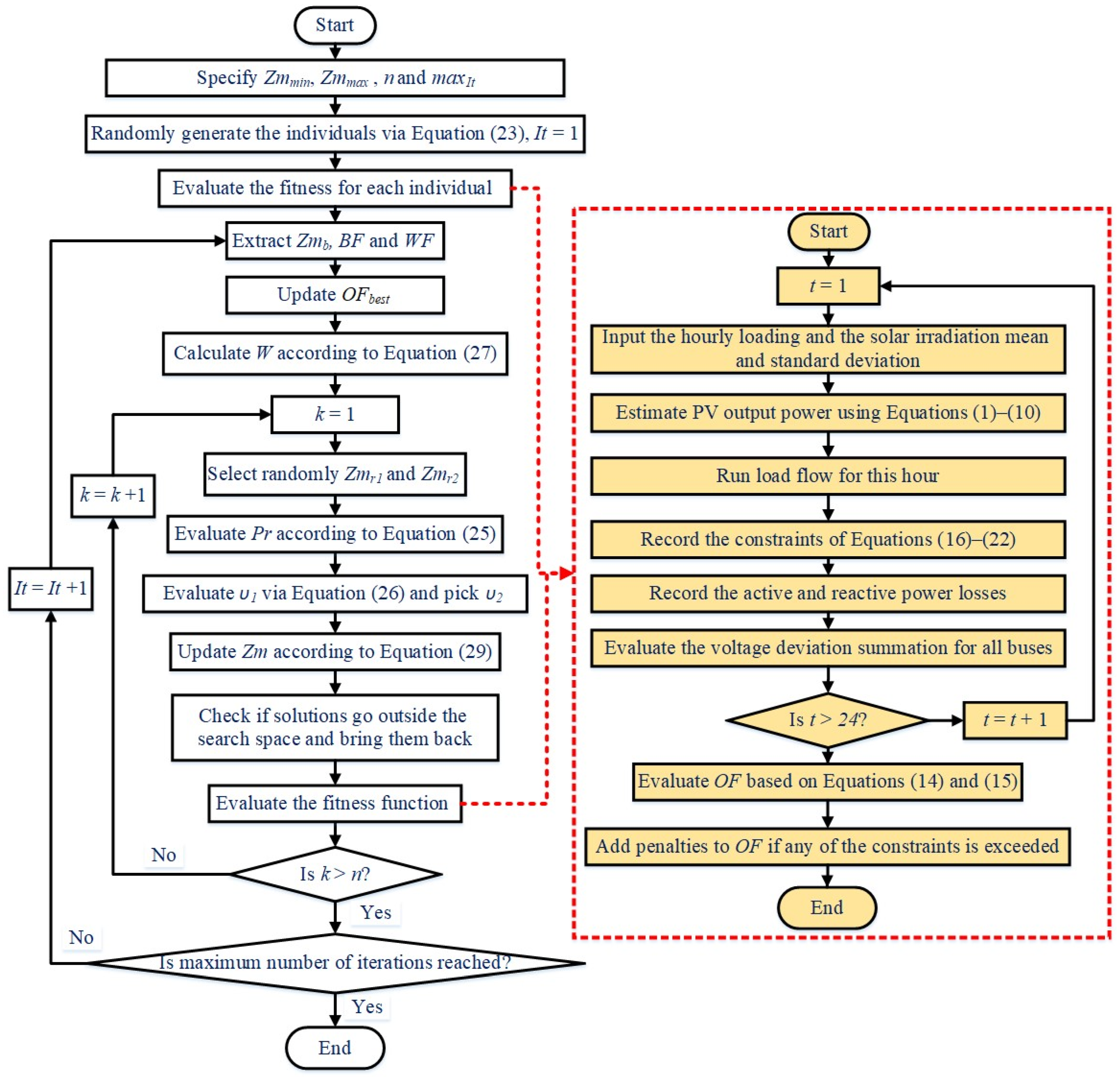
To handle the proposed formulation described in the previous section, Figure 1 displays the developed SMA for the allocation of PVDGs with Volt/Var control based on AVR in distribution networks.
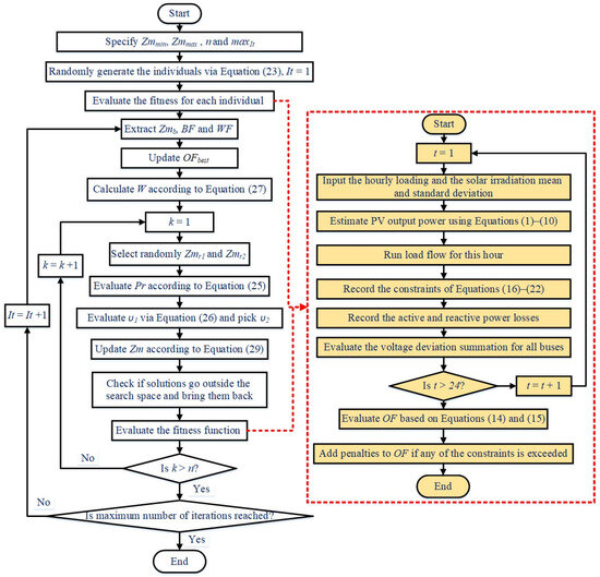
Figure 1.
Developed SMA for allocation of PVDGs with Volt/Var control based on AVR in distribution networks.
As shown, each solution vector (Zm) is represented by the candidate buses to install PVDGs, their sizes and the hourly tap settings as stated in Equation (13). The solution vectors are randomly initialized using Equation (23) to compose the population. Then, the fitness function of Equation (14) is evaluated where each hourly loading is simulated. For each hour, Input the hourly solar irradiation mean and the standard deviation is considered based on the historic data, and the PV output power is estimated considering the associated uncertainties. Therefore, the load flow algorithm [50] for each hour and the active and reactive power losses, and the system constraints of Equations (16)–(22) are recorded while the voltage deviation summation for all buses is evaluated. After finishing the simulation for all 24 h, the three indices of Equation (15) are estimated and therefore the objective function of Equation (14) is accomplished. Based on the recorded constraints, the violated constraints are penalized by adding penalty components to the objective function. Across all solutions, the minimum objective value will be extracted as the best one with (OFbest). After that, the SMA updating mechanism is working to generate the new updated solutions using Equation (29). The new solution vectors are maintained within their permissible ranges and the objective function will be evaluated as described before. Then, the best solution with the minimum objective value will be updated (OFbest). This process is repeated until the whole number of iterations is completed.
4. Simulation Results and Discussions
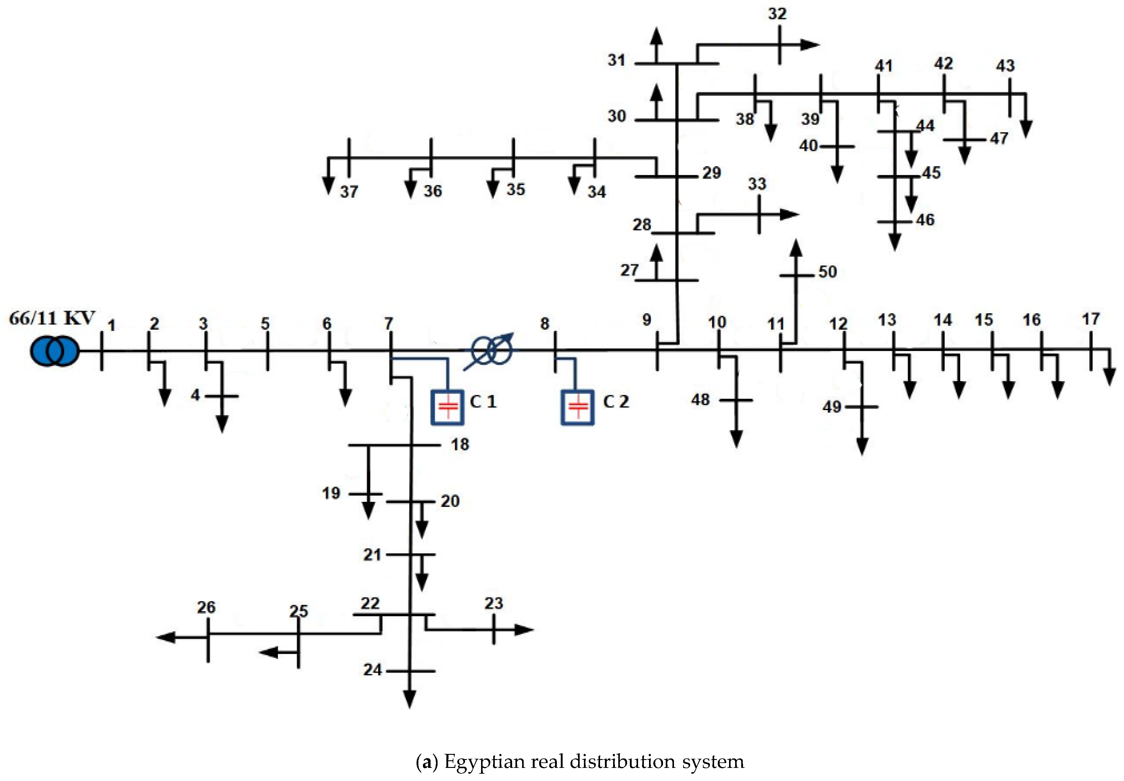
In this study, two practical distribution networks are selected. The first is the Kafr Rabea feeder in the Menoufia governorate which belongs to the South Delta Electricity Company. The first system is a real Egyptian distribution system which consists of 50 nodes with 49 lines and has 2.294 MW and 1.1 MVAr, and its rated voltage is 11 kV. The second system consists of 141 nodes with 140 lines and has 12.19 MW and 6.289 MVAr and its rated voltage is 12.47 kV. The line and load data of the first system are obtained from [50]. The second is related to the metropolitan area of Caracas. The single-line diagrams of both networks are shown in Figure 2. The proposed methodology is coded using MATLAB 2020a and the simulation results are acquired via a DELL laptop with Intel R Processor Core(TM) i7-10750H CPU @ 2.60 GHz with 16.0 GB of RAM.


Figure 2.
Single-line diagram of the two studied systems.
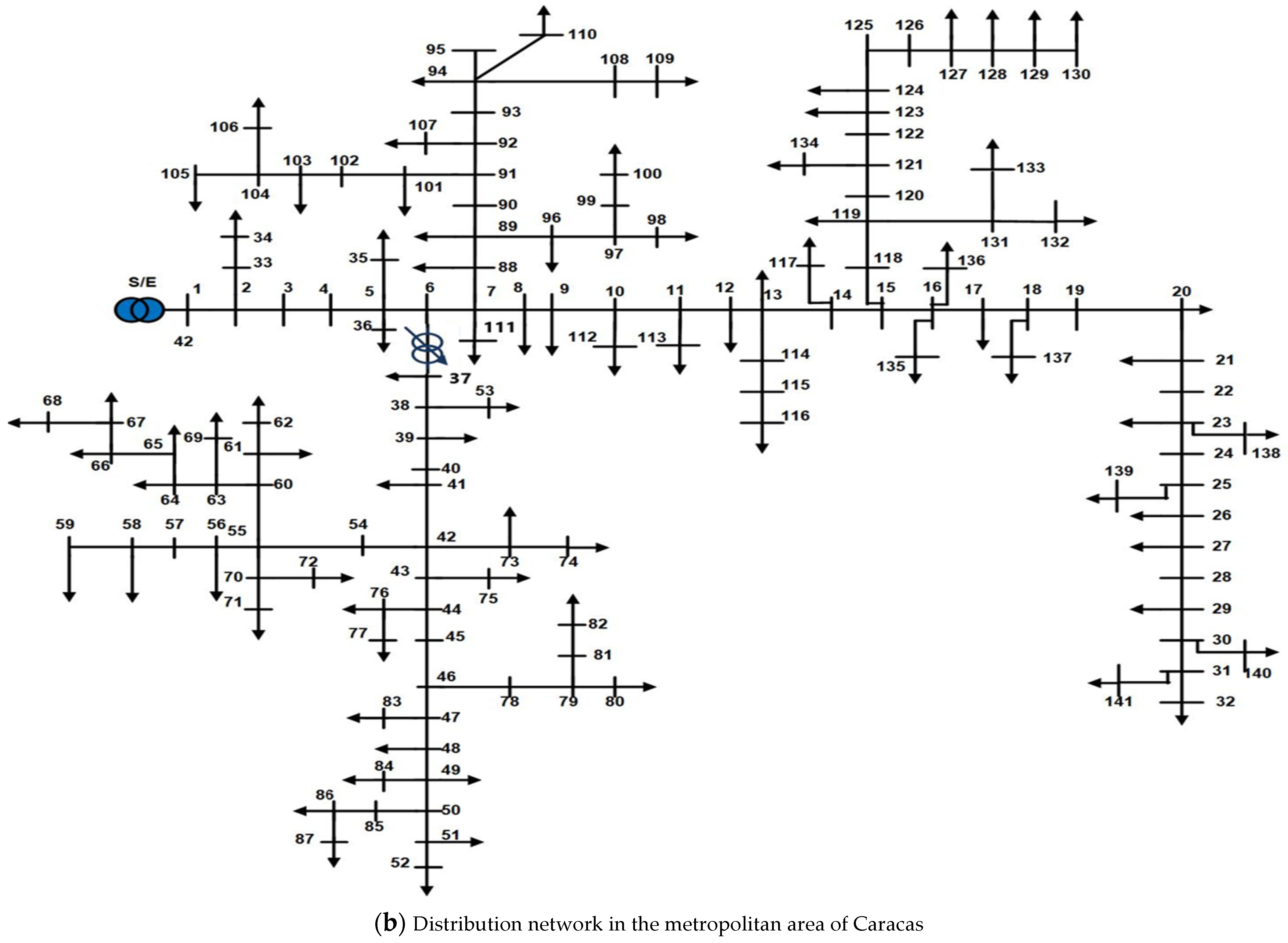
Taking solar radiation uncertainties into account, the PDF for 20 solar irradiance states with an interval of 0.05 kW/m2 for hours 6–19 is generated and the hourly expected output of the PVDGs is estimated as displayed in Figure 3. The solar irradiance varies with time and weather; hence, it is obvious that different periods have varied PDFs. Each hour’s area under the curve is one. The maximum expected output powers exist among hours 11–14. This is due to the dependence of the PV output on the ambient temperature, solar irradiance, and the PV module characteristics. The total expected output power per hour can be calculated as the sum of all the expected output powers at that hour.
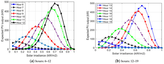
Figure 3.
Expected PVDG output for hours.
4.1. Simulation Results for the First Practical System
The performance of the distribution system in terms of the active and reactive power loss indices and system voltage deviation is assessed considering the uncertainties of PV output power. In addition, the load profile per day is considered where hourly load variations are addressed as [50]. For this system, an AVR having a 400 Ampere size linked between buses 7–8 and two capacitors at nodes 7 and 8 with nominal sizes of 300 kVAr each are taken into consideration. The minimum limit of the voltage value to be considered is 0.9 per unit (PU) [50]. Three case studies are considered to analyze the impacts of allocation of PVDGs with Volt/Var control based on AVR management for their tap positions as follows:
- Case 1: Allocation of PVDGs and AVR tap positions considering unity power factors operation for the PVDG.
- Case 2: Analyzing the impacts of the variation of lag power factors operation for the PVDG simultaneously with AVR control.
- Case 3: Investigating the impacts of optimal allocation of different numbers of PVDGs with two different power factors’ operation and AVR control.
4.1.1. Case 1
In the first case, the PVDG operation mode is running with unity power factors where they are capable of injecting active power only. The proposed SMA algorithm is applied for allocation of PVDGs and AVR tap positions while four PVDGs are to be installed. To evaluate the computing effectiveness of the applied SMA, different recent algorithms are used such as artificial rabbits optimization (ARO) (ARO) [37], grey wolf optimizer (GWO) [38], and particle swarm optimization (PSO) [39]. They are applied with the same circumstances: the population is 30; number of iterations is 80; and number of run times is 20. Through all separate runs, the best obtained allocation option of PVDGs for each algorithm is tabulated in Table 1 which records the sizes and nodes to install the PVDGs, the three system indices and the objective value. Simultaneously, Figure 4 shows the associated daily variation of AVR tap positions for each algorithm. From Table 1, the results of the optimization process demonstrate the superior ability of the SMA in comparison with ARO, GWO, and PSO to achieve the best objective function value of 13.648 PU. The SMA selects the nodes 30, 34, 15, and 32 to install 500, 10, 500, and 499 kW, respectively. Also, the AVR tap position is controlled in each hour as displayed in Figure 4a where the SMA raises the tap positions more than step 4 through the day. This figure indicates that the AVR tap position varies each hour due to daily load variation to improve system bus voltages. After that, PSO minimizes the considered objective to 13.8669 PU while ARO and GWO obtain objectives of 14.3085 and 14.633 PU, respectively. The SMA is the best performance. Considering the objective value, the SMA achieves improvement with 4.62, 6.73, and 1.58%, respectively, compared to ARO, GWO, and PSO. On the level of the active power loss index, the SMA achieves improvement with 1.5, 0.93, and 0.64%, respectively, compared to ARO, GWO and PSO. For the reactive power loss index, the SMA achieves improvement with 0.7, 0.82 and 1.02%, respectively, compared to ARO, GWO, and PSO. Considering the minimum objective value, the SMA achieves improvement with 20.05, 29.98, and 5.91%, respectively, compared to ARO, GWO, and PSO.

Table 1.
Best obtained results of each algorithm for the allocation of four PVDGs for the first system.
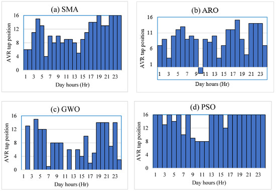
Figure 4.
Optimal AVR tap position considering the hourly load variations for each algorithm.
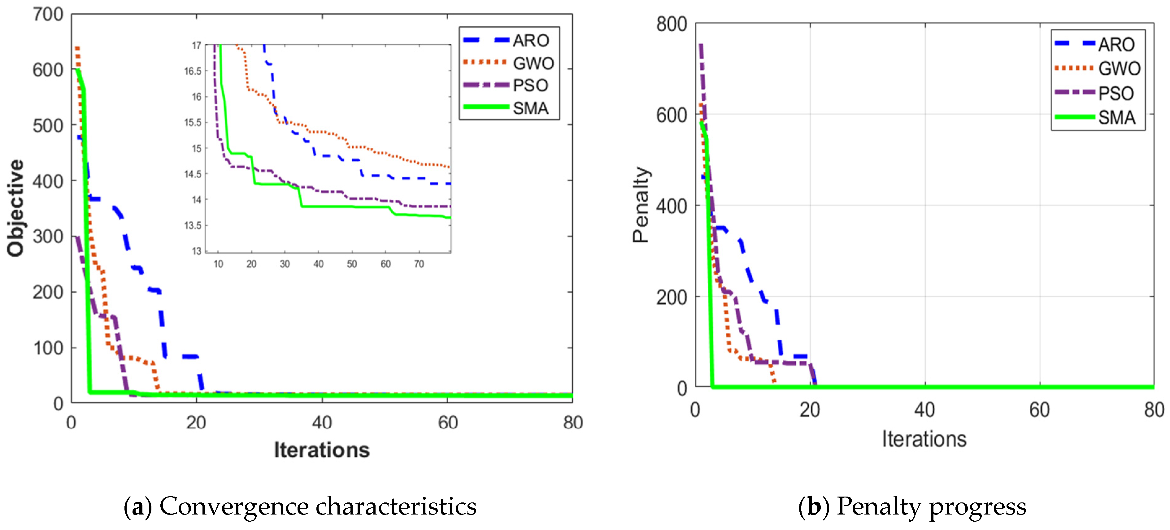
Figure 5 displays the convergence characteristics and penalty curves of the different applied algorithms in this case. As shown in Figure 5a, the SMA provides better evolution towards the minimum objective and faster convergence than the other algorithms. Added to that, from Figure 5b, the penalty values are decreasing and approaching zero for all the applied techniques which indicates that the constraints are completely maintained. Also, this figure proves the faster convergence of the SMA where the zero penalty is achieved at only five iterations whereas GWO, PSO, and ARO achieve the zero penalty at iterations 16, 21, and 22, respectively.
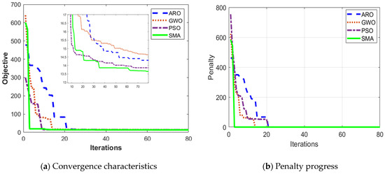
Figure 5.
Convergence characteristics and penalty curves of the compared algorithms for case 1.
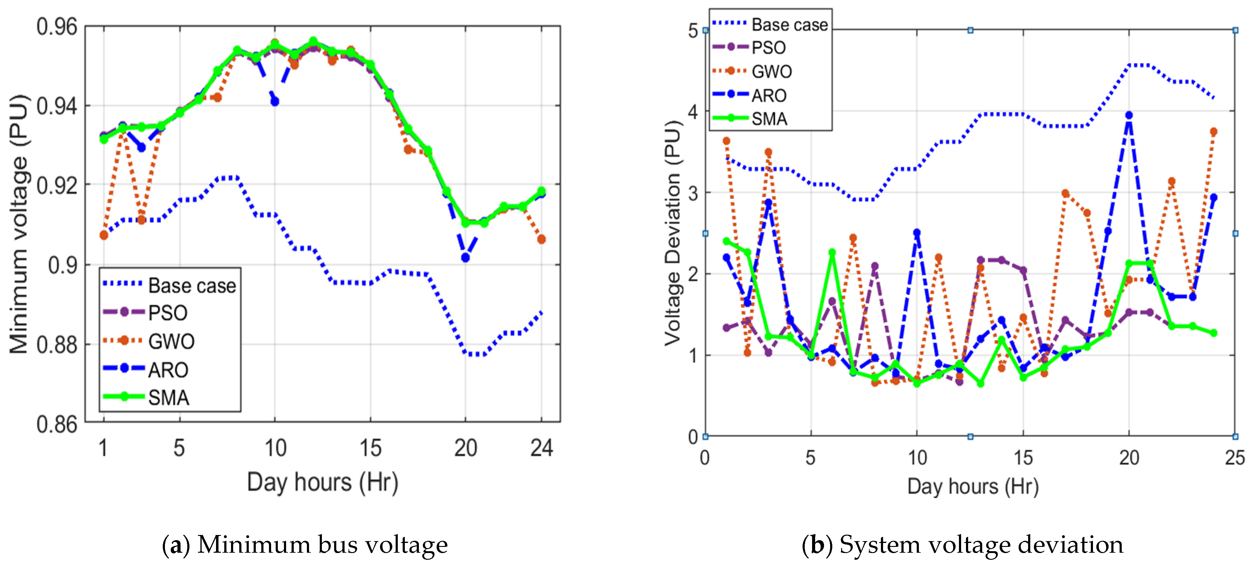
Moreover, Figure 6 illustrates the hourly variations of the minimum bus voltage and system voltage deviations. As shown, the minimum bus voltage is greatly improved during all day hours with optimal integration of PVDGs into the system with AVR control compared to the system base case. The proposed SMA algorithm is successfully improving the minimum bus voltage compared to the others since it approximately achieves higher voltage values throughout the day. Similarly, great reductions in the system voltage deviation during all day hours compared to the system base case. The highest reduction in the system voltage deviation is according to the proposed SMA algorithm compared to the other algorithms.
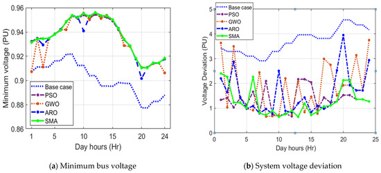
Figure 6.
Hourly variations of the minimum voltage and the whole voltage deviation.
4.1.2. Case 2
In the second case, the impacts of scheduled power factor variation of PVDGs on the optimal allocation of PVDGs and AVR control are investigated. Therefore, PVDGs are capable to inject active power and reactive power which is determined based on the scheduled power factor. The power factor varies from unity to 0.8 lagging by step 0.05. The proposed SMA algorithm is applied for allocation of PVDGs and AVR tap positions while four PVDGs are to be installed and Table 2 indicates the impacts on the system’s active and reactive power loss and voltage deviation indices. Also, the accompanied AVR tap position in each hour is displayed in Figure 7.
Table 2.
SMA application for allocation of four PVDGs with AVR control with different scheduled power factors.
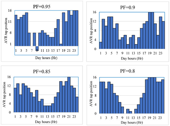
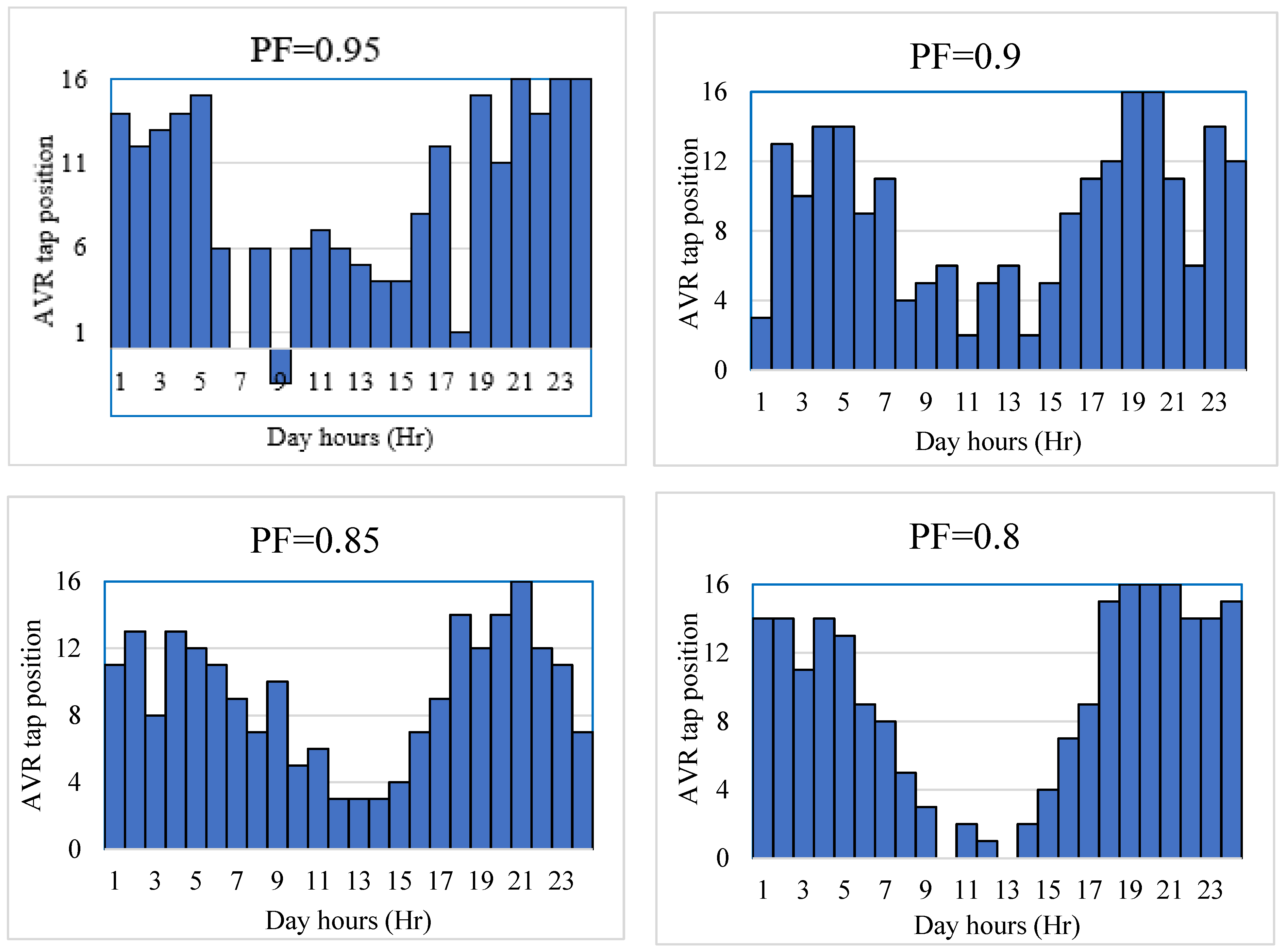
Figure 7.
Hourly variation of AVR tap position with scheduled PVDG power factor variation based on SMA.
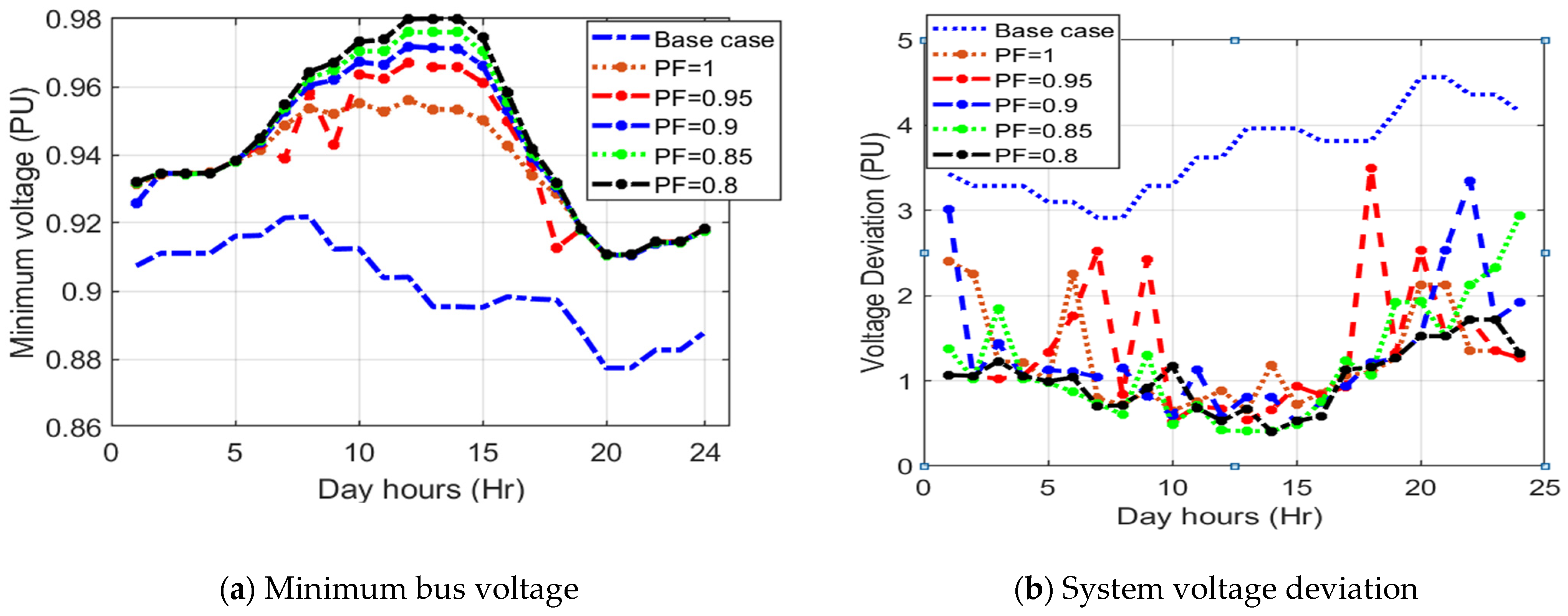
From Table 2 and Figure 7, as the scheduled power factor is decreased, the system performance indices are improved. Compared to the unity power factor operation mode, the reduction percentage in the optimization objective is 1.58%, 2.28%, 2.85%, and 3.99% according to 0.95, 0.9, 0.85, and 0.8 PVDGs power factors, respectively. In addition, Figure 7 shows the significant controllability of the AVR since its tap position drops when PVDG output is abundant during the hours of sunshine from 7 to 18 o’clock approximately. During these hours, there is a high increase in the produced reactive power from PVDGs, especially with lower scheduled power factors, and consequently, the AVR tap position decreases to improve the voltage profile in the whole system. This result is confirmed by Figure 8 which indicates the hourly variation of system bus voltage and voltage deviation with scheduled PVDG power factor variation based on SMA. From Figure 8, the minimum bus voltage and the system voltage deviation are greatly improved during all day hours under different scheduled power factors compared to the system base case.

Figure 8.
Hourly variations of the minimum voltage and the voltage deviation with different scheduled power factors.
4.1.3. Case 3
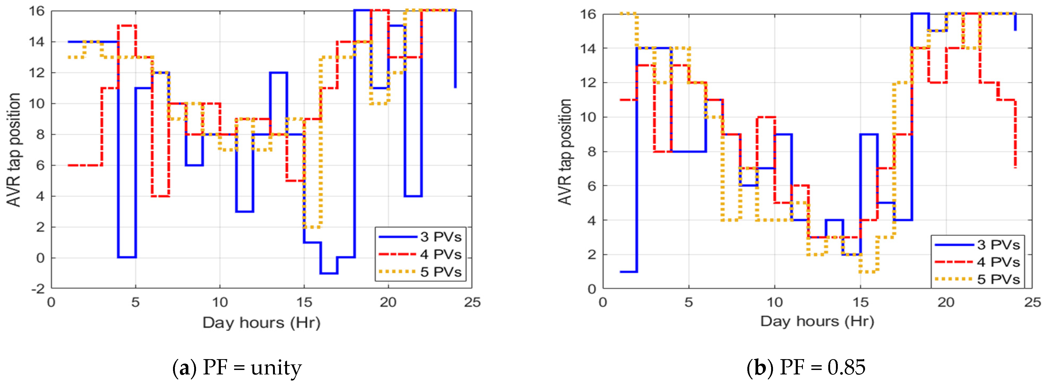
The impacts of optimal allocation of PVDGs and AVR tap positions under different numbers of PVDGs are investigated. For this purpose, three, four, and five PVDGs are considered at two different scheduled power factors of 1 and 0.85. The proposed SMA has been applied and the simulation results for the optimal location and size of PVDG are shown in Table 3 while Figure 9 displays the associated optimal hourly variations of AVR tap position with different numbers of PVDGs.
Table 3.
Results of SMA for optimal allocation of different numbers of PVDG units with different power factors.
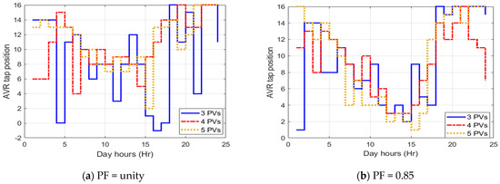
Figure 9.
Optimal hourly variation of AVR tap position with different numbers of PVDG units based on SMA.
The table results illustrate that:
- The active power loss index decreased by about 0.75% and 1.54% when using four and five units compared with the case of three units at unity PF, while that index reduction is 3.89% and 5.11% when using four and five units compared with the case of three units at 0.85 PF lagging.
- Similarly, the reactive power loss index decreased by about 0.65% and 1.29% with four and five units at unity PF, while that index reduction is 4% and 4.77% at 0.85 PF lagging.
- Also, the voltage deviation index decreased by about 20.94% and 28.94% when using four and five units at unity PF, while that index reduction is 11.01% and 19.44% when using four and five units at 0.85 PF lagging.
- The improvement in the whole objective function is about 4.4% and 6.47% with four and five installed PVDGs compared to three units at unity PF. The improvements are 5.01% and 7.19% at 0.85 PF lagging.
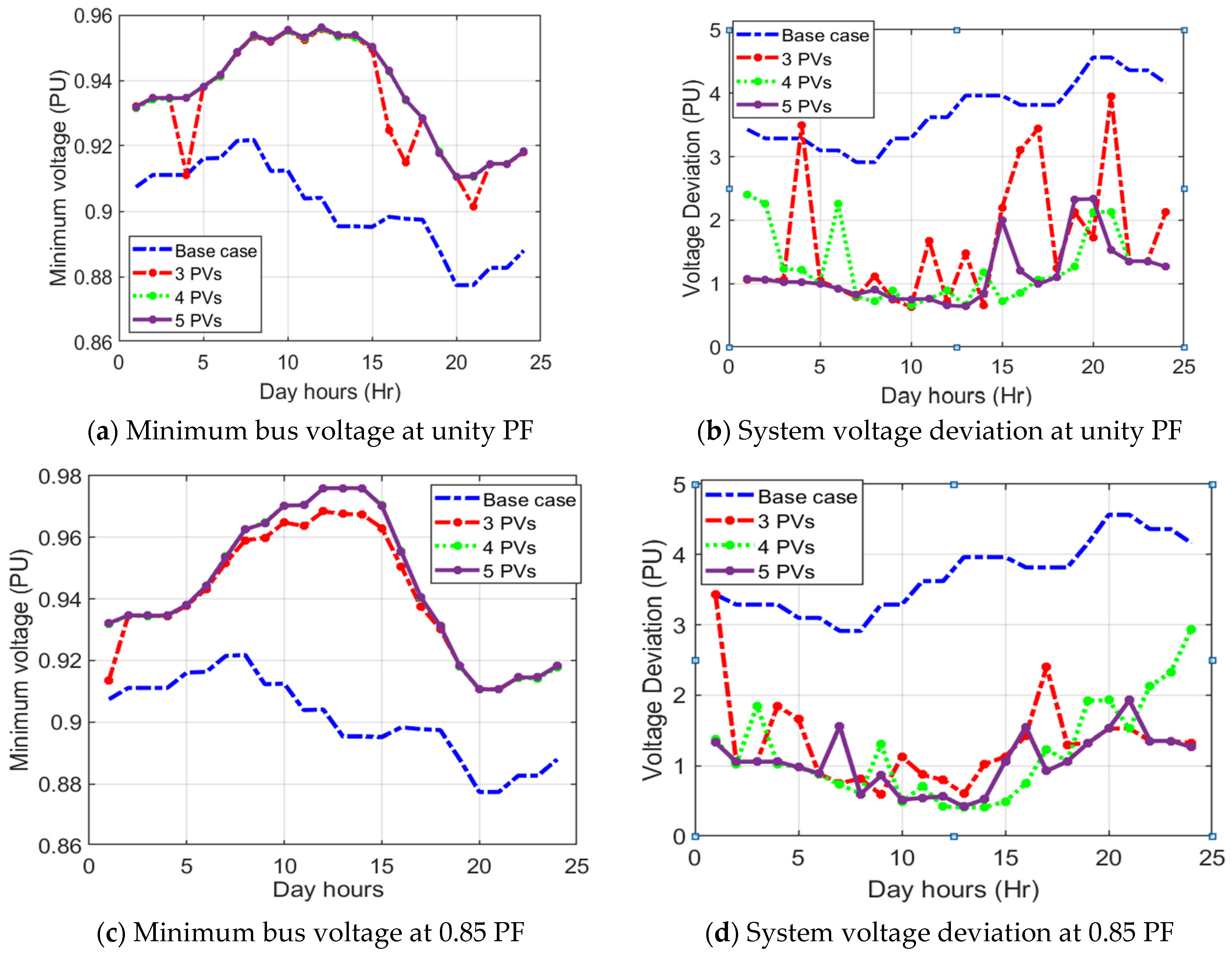
An additional capability of reactive power injection has a great impact on the losses and the voltage profile where the system performance indices are improved at 0.85 PF lagging than unity PF at the same integrating numbers of PVDGs into the studied system. From Figure 9, the optimal tap positions are decreased during the period of sunshine from 7 to 19 o’clock. By comparing the tap position in the two cases, namely unity PF and 0.85 PF in these hours, the specified steps of the tap positions in the case of 0.85 PF are much less than their counterparts in the case of unity PF. This decrease is due to the presence of an abundance of solar cell output power, especially reactive power. Additionally, Figure 10 indicates a significant reduction in the minimum bus voltage and the system voltage deviation at 0.85 PF lagging compared to the unity PF, respectively. Both scheduled power factors derive higher improvement compared to the base case.
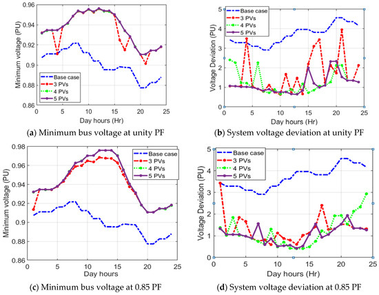
Figure 10.
Hourly variation of the minimum bus voltage and system voltage deviation under different numbers of PVDGs units at unity PF based on SMA.
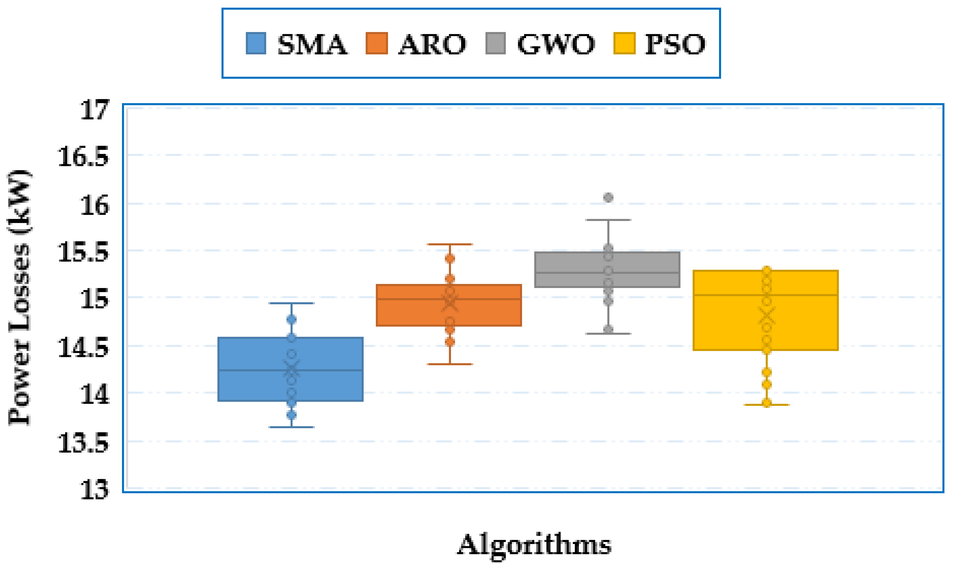
4.1.4. Statistical Analysis of the Compared Algorithms for This System
There is no guarantee for any optimization algorithm to obtain the global optimal solution but, these drawbacks can be addressed by implementing statistical results on each optimization technique. Each technique is executed for twenty different separate runs and the accuracy of each technique is carried out by obtaining minimum, maximum, mean value, and standard deviation. Figure 11 displays the box plot of the obtained power losses of the SMA, ARO, GWO, and PSO for the first system while their statistical comparisons are tabulated in Table 4. As shown, in comparison to all compared methods, the SMA demonstrates the lowest best, mean and worst of the obtained losses of 13.64801, 14.2631 and 14.93856 kW, respectively. Based on the SMA technique, the closer the mean value is to the best and worst, and the standard deviation is the minimum, the more evidence and indication of the strength of this method.
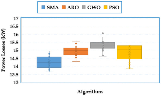
Figure 11.
Statistical comparisons of the outcomes of SMA, ARO, GWO, and PSO for the first system.
Table 4.
Statistical metrics of the compared algorithms for the first system.
4.2. Simulation Results for the Second Practical System
For the second practical system of the metropolitan area of Caracas, the proposed SMA is applied to find the optimal allocation of PVDGs and AVR tap positions. For hourly load variations, the optimal allocation of six PVDGs, as well as the optimal AVR tap positions were found considering the change in the scheduled power factor of the PVDGs as displayed in Table 5 and Figure 12. As shown, it is evident that the objective function decreases with the increase in PVDG’s power factor, due to the increase in the reactive power injections to the system. The reduction percentage in the objective function reaches 1.39%, 2.28%, 2.44%, and 2.58% for 0.95, 0.9, 0.85, and 0.8 PF lagging, respectively, compared with the case of unity PF. Also, the system variations in terms of the minimum bus voltage and voltage deviation have been observed as shown in Figure 13. As shown, significant improvement in the minimum bus voltage during all-day hours especially the peak loading hours using PVDG units with any power factor value and using the AVR control where its value is greater than 95% during all-day hours. Also, system voltage deviation is decreased by a large value compared to the base case. The best performance of the system is the state of 0.85 PF lagging in that it is the highest low voltage as well as the lowest voltage deviation throughout the hours of the day.
Table 5.
Results of SMA for optimal allocation of six PVDG units with a different power factor of PVDGs.
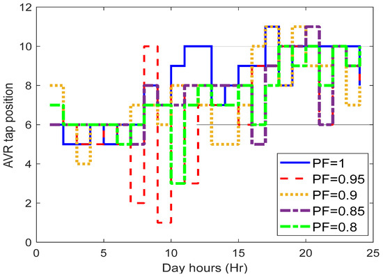
Figure 12.
Optimal daily variation of AVR tap position with scheduled PVDGs power factor variation based on SMA.
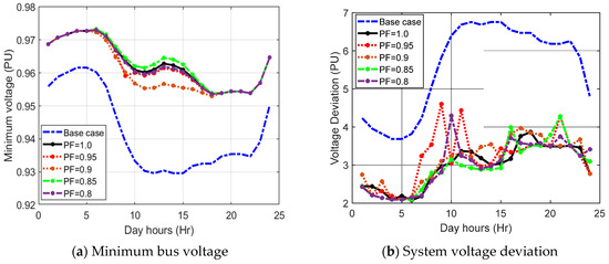
Figure 13.
Hourly variations of minimum voltage and voltage deviations with a different power factor of PVDGs.
Additionally, the impacts of optimal allocation of PVDG units with different power factors and optimal AVR tap positions are investigated on system active and reactive power losses as in Figure 14. The reductions in system active and reactive power losses are great compared with the base case, especially the loading peak hours. It also shows that PVDG units with a unity power factor represent the least improvement in the system’s performance.
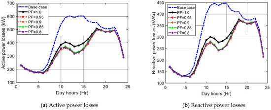
Figure 14.
Hourly variations of system losses with different power factor of PVDGs.
5. Conclusions
This study presents a developed methodology based on SMA for the optimal location and size of the PVDG energy resources with simultaneous Volt/Var control via optimal settings of the AVR tap positions. The study objectives are to minimize active and reactive power losses and enhance the voltage quality in the studied networks. The PVDG uncertainty and the hourly load variations have been taken into the optimization frame. The simulation implementations are executed on two practical distribution networks which are the Kafr Rabea area related to South Delta Electricity Company in Egypt and a large-scale distribution network from the metropolitan area of Caracas. For solving the proposed optimization framework, the developed SMA provides superior performance over ARO, GWO, and PSO in minimizing the active and reactive power losses and improving the voltage profile where it provides better evolution towards the minimum objective and faster convergence than the other algorithms. Also, the AVR tap position varies each hour due to the load variations to improve system bus voltages. The minimum bus voltage and the system voltage deviation are greatly improved during all day hours with optimal integration of PVDGs into the system with AVR control compared to the system base case for the two studied networks. As the scheduled power factor of the PVDGs is decreased, the system performance indices are improved. The significant controllability of the AVR since its tap position drops when PVDG output is abundant during the hours of sunshine from 7 to 18 o’clock approximately. More enhancement in the system performance indices has been achieved by increasing the number of PVDGs. There is some limitation to the proposed methodology in that the studied systems are balanced and do not take the unbalanced model so this is an extension to this work in the future.
Author Contributions
Conceptualization, A.M.S. and A.F.N.; Methodology, A.M.S.; Software, A.M.S. and A.F.N.; Validation, A.M.S.; Formal analysis, E.E.E. and N.A.N.; Investigation, E.E.E.; Data curation, A.F.N.; Writing—original draft, A.F.N.; Writing—review & editing, N.A.N.; Supervision, E.E.E. All authors have read and agreed to the published version of the manuscript.
Funding
This work is funded by the Deanship of Scientific Research, Taif University.
Institutional Review Board Statement
Not applicable.
Informed Consent Statement
Not applicable.
Data Availability Statement
The data presented in this study are available on request from the corresponding author.
Acknowledgments
The researchers would like to acknowledge the Deanship of Scientific Research, Taif University, for funding this work.
Conflicts of Interest
The authors declare no conflict of interest.
References
- IRENA. Future of Wind (Deployment, Investment, Technology, Grid Integration and Socio-Economic Aspects); IRENA: Masdar City, United Arab Emirates, 2019. [Google Scholar]
- Abbasi, F.; Hosseini, S.M. Optimal DG Allocation and Sizing in Presence of Storage Systems Considering Network Configuration Effects in Distribution Systems. IET Gener. Transm. Distrib. 2016, 10, 617–624. [Google Scholar] [CrossRef]
- Holjevac, N.; Baškarad, T.; Ðaković, J.; Krpan, M.; Zidar, M.; Kuzle, I. Challenges of High Renewable Energy Sources Integration in Power Systems—The Case of Croatia. Energies 2021, 14, 1047. [Google Scholar] [CrossRef]
- Huang, D.; Li, H.; Cai, G.; Huang, N.; Yu, N.; Huang, Z. An Efficient Probabilistic Approach Based on Area Grey Incidence Decision Making for Optimal Distributed Generation Planning. IEEE Access 2019, 7, 93175–93186. [Google Scholar] [CrossRef]
- Shafiul Alam, M.; Al-Ismail, F.S.; Salem, A.; Abido, M.A. High-Level Penetration of Renewable Energy Sources into Grid Utility: Challenges and Solutions. IEEE Access 2020, 8, 190277–190299. [Google Scholar] [CrossRef]
- Ahmadi, B.; Ceylan, O.; Ozdemir, A. Reinforcement of the Distribution Grids to Improve the Hosting Capacity of Distributed Generation: Multi-Objective Framework. Electr. Power Syst. Res. 2023, 217, 109120. [Google Scholar] [CrossRef]
- Borousan, F.; Hamidan, M.A. Distributed Power Generation Planning for Distribution Network Using Chimp Optimization Algorithm in Order to Reliability Improvement. Electr. Power Syst. Res. 2023, 217, 109109. [Google Scholar] [CrossRef]
- Moghaddam, M.J.H.; Kalam, A.; Shi, J.; Nowdeh, S.A.; Gandoman, F.H.; Ahmadi, A. A New Model for Reconfiguration and Distributed Generation Allocation in Distribution Network Considering Power Quality Indices and Network Losses. IEEE Syst. J. 2020, 14, 3530–3538. [Google Scholar] [CrossRef]
- Fan, V.H.; Dong, Z.; Meng, K. Integrated Distribution Expansion Planning Considering Stochastic Renewable Energy Resources and Electric Vehicles. Appl. Energy 2020, 278, 115720. [Google Scholar] [CrossRef]
- Hadidian-Moghaddam, M.J.; Arabi-Nowdeh, S.; Bigdeli, M.; Azizian, D. A Multi-Objective Optimal Sizing and Siting of Distributed Generation Using Ant Lion Optimization Technique. Ain Shams Eng. J. 2018, 9, 2101–2109. [Google Scholar] [CrossRef]
- Petinrin, J.O.; Shaabanb, M. Impact of Renewable Generation on Voltage Control in Distribution Systems. Renew. Sustain. Energy Rev. 2016, 65, 770–783. [Google Scholar] [CrossRef]
- Kashyap, M.; Kansal, S.; Verma, R. Sizing and Allocation of DGs in A Passive Distribution Network Under Various Loading Scenarios. Electr. Power Syst. Res. 2022, 209, 108046. [Google Scholar] [CrossRef]
- Zhang, D.; Li, J.; Hui, D. Coordinated Control for Voltage Regulation of Distribution Network Voltage Regulation by Distributed Energy Storage Systems. Prot. Control Mod. Power Syst. 2018, 3, 3. [Google Scholar] [CrossRef]
- Girisha, K.M.; Kumar, N. Optimal Allocation of Multiple Distributed Generators for Network Loss Reduction & Voltage Profile Improvement. Int. J. Emerg. Technol. Comput. Sci. Electron. 2016, 23, 2091668. [Google Scholar]
- Duong, M.; Pham, T.; Nguyen, T.; Doan, A.; Tran, H. Determination of Optimal Location and Sizing of Solar Photovoltaic Distribution Generation Units in Radial Distribution Systems. Energies 2019, 12, 174. [Google Scholar] [CrossRef]
- Moustafa, G.; Elshahed, M.; Ginidi, A.R.; Shaheen, A.M.; Mansour, H.S.E. A Gradient-Based Optimizer with a Crossover Operator for Distribution Static VAR Compensator (D-SVC) Sizing and Placement in Electrical Systems. Mathematics 2023, 11, 1077. [Google Scholar] [CrossRef]
- Zellagui, M.; Belbachir, N.; El-Sehiemy, R.A.; El-Bayeh, C.Z. Multi-Objective Optimal Allocation of Hybrid Photovoltaic Distributed Generators and Distribution Static Var Compensators in Radial Distribution Systems Using Various Optimization Algorithms. J. Electr. Syst. 2022, 18, 1–22. [Google Scholar]
- Wang, W.; Yu, N.; Shi, J.; Gao, Y. Volt-VAR Control in Power Distribution Systems with Deep Reinforcement Learning. In Proceedings of the 2019 IEEE International Conference on Communications, Control, and Computing Technologies for Smart Grids (SmartGridComm), Beijing, China, 21–23 October 2019. [Google Scholar]
- Malekpour, A.R.; Annaswamy, A.M.; Shah, J. Hierarchical Hybrid Architecture for Volt/Var Control of Power Distribution Grids. IEEE Trans. Power Syst. 2020, 35, 854–863. [Google Scholar] [CrossRef]
- Baran, M.; Wu, F.F. Optimal Sizing of Capacitors Placed on a Radial Distribution System. IEEE Trans. Power Deliv. 1989, 4, 735–743. [Google Scholar] [CrossRef]
- Devabalaji, K.R.; Ravi, K.; Kothari, D.P. Optimal Location and Sizing of Capacitor Placement in Radial Distribution System Using Bacterial Foraging Optimization Algorithm. Int. J. Electr. Power Energy Syst. 2015, 71, 383–390. [Google Scholar] [CrossRef]
- Injeti, S.K.; Thunuguntla, V.K.; Shareef, M. Optimal Allocation of Capacitor Banks in Radial Distribution Systems for Minimization of Real Power Loss and Maximization of Network Savings Using Bio-Inspired Optimization Algorithms. Int. J. Electr. Power Energy Syst. 2015, 69, 441–455. [Google Scholar] [CrossRef]
- Zeraati, M.; Golshan, M.E.H.; Guerrero, J.M. A Consensus-Based Cooperative Control of PEV Battery and PV Active Power Curtailment for Voltage Regulation in Distribution Networks. IEEE Trans. Smart Grid 2017, 10, 670–680. [Google Scholar] [CrossRef]
- Wang, Y.; Xu, Y.; Tang, Y.; Syed, M.H.; Guillo-Sansano, E.; Burt, G.M. Decentralised-Distributed Hybrid Voltage Regulation of Power Distribution Networks Based on Power Inverters. IET Gener. Transm. Distrib. 2019, 13, 444–451. [Google Scholar]
- Karmakar, N.; Bhattacharyya, B. Hybrid Intelligence Approach for Multi-Load Level Reactive Power Planning Using VAR Compensator in Power Transmission Network. Prot. Control Mod. Power Syst. 2021, 6, 26. [Google Scholar] [CrossRef]
- Pereira, L.D.L.; Yahyaoui, I.; Fiorotti, R.; de Menezes, L.S.; Fardin, J.F.; Rocha, H.R.O.; Tadeo, F. Optimal Allocation of Distributed Generation and Capacitor Banks Using Probabilistic Generation Models with Correlations. Appl. Energy 2022, 307, 118097. [Google Scholar] [CrossRef]
- Shaheen, A.; El-Seheimy, R.; Kamel, S.; Selim, A. Reliability Enhancement and Power Loss Reduction in Medium Voltage Distribution Feeders Using Modified Jellyfish Optimization. Alex. Eng. J. 2023, 75, 363–381. [Google Scholar] [CrossRef]
- Shiratsuchi, N.; Hirano, M. Techniques for Each Problem of the Voltage Regulator for Distribution Line, and Their Advantages and Disadvantages Evaluation. IEEJ Trans. Power Energy 2020, 140, 465–473. [Google Scholar] [CrossRef]
- dos Santos Pereira, G.M.; Fernandes, T.S.P.; Aoki, A.R. Allocation of Capacitors and Voltage Regulators in Three-Phase Distribution Networks. J. Control Autom. Electr. Syst. 2018, 29, 238–249. [Google Scholar] [CrossRef]
- Chamana, M.; Chowdhury, B.H. Optimal Voltage Regulation of Distribution Networks With Cascaded Voltage Regulators in the Presence of High PV Penetration. IEEE Trans. Sustain. Energy 2018, 9, 1427–1436. [Google Scholar] [CrossRef]
- Liu, Y.; Li, J.; Wu, L. Coordinated Optimal Network Reconfiguration and Voltage Regulator/DER Control for Unbalanced Distribution Systems. IEEE Trans. Smart Grid 2019, 10, 2912–2922. [Google Scholar] [CrossRef]
- Khunkitti, S.; Siritaratiwat, A.; Premrudeepreechacharn, S. Multi-Objective Optimal Power Flow Problems Based on Slime Mould Algorithm. Sustainability 2021, 13, 7448. [Google Scholar] [CrossRef]
- Hassan, M.H.; Kamel, S.; Abualigah, L.; Eid, A. Development and Application of Slime Mould Algorithm for Optimal Economic Emission Dispatch. Expert Syst. Appl. 2021, 182, 115205. [Google Scholar] [CrossRef]
- Yu, K.; Liu, L.; Chen, Z. An Improved Slime Mould Algorithm for Demand Estimation of Urban Water Resources. Mathematics 2021, 9, 1316. [Google Scholar] [CrossRef]
- Nguyen, T.T.; Wang, H.J.; Dao, T.K.; Pan, J.S.; Liu, J.H.; Weng, S. An Improved Slime Mold Algorithm and Its Application for Optimal Operation of Cascade Hydropower Stations. IEEE Access 2020, 8, 226754–226772. [Google Scholar] [CrossRef]
- Dhawale, D.; Kamboj, V.K.; Anand, P. An Effective Solution to Numerical and Multi-Disciplinary Design Optimization Problems Using Chaotic Slime Mold Algorithm. Eng. Comput. 2021, 38, 2739–2777. [Google Scholar] [CrossRef]
- Wang, L.; Cao, Q.; Zhang, Z.; Mirjalili, S.; Zhao, W. Artificial Rabbits Optimization: A New Bio-Inspired Meta-Heuristic Algorithm for Solving Engineering Optimization Problems. Eng. Appl. Artif. Intell. 2022, 114, 105082. [Google Scholar] [CrossRef]
- Faris, H.; Aljarah, I.; Al-Betar, M.A.; Mirjalili, S. Grey Wolf Optimizer: A Review of Recent Variants and Applications. Neural Comput. Appl. 2018, 30, 413–435. [Google Scholar]
- Kennedy, J.; Eberhart, R. Particle Swarm Optimization. In Proceedings of the ICNN’95—International Conference on Neural Networks, Perth, WA, Australia, 27 November–1 December 1995. [Google Scholar]
- Salameh, Z.M.; Borowy, B.S.; Amin, A.R.A. Photovoltaic Module-Site Matching Based on the Capacity Factors. IEEE Trans. Energy Convers. 1995, 10, 326–332. [Google Scholar] [CrossRef]
- Khatod, D.K.; Pant, V.; Sharma, J. Evolutionary Programming Based Optimal Placement of Renewable Distributed Generators. IEEE Trans. Power Syst. 2013, 28, 683–695. [Google Scholar] [CrossRef]
- Atwa, Y.M.; El-Saadany, E.F.; Salama, M.M.A.; Seethapathy, R. Optimal Renewable Resources Mix for Distribution System Energy Loss Minimization. IEEE Trans. Power Syst. 2010, 25, 360–370. [Google Scholar] [CrossRef]
- Teng, J.H.; Luan, S.W.; Lee, D.J.; Huang, Y.Q. Optimal Charging/Discharging Scheduling of Battery Storage Systems for Distribution Systems Interconnected with Sizeable PV Generation Systems. IEEE Trans. Power Syst. 2013, 28, 1425–1433. [Google Scholar] [CrossRef]
- Soroudi, A.; Aien, M.; Ehsan, M. A Probabilistic Modeling of Photo Voltaic Modules and Wind Power Generation Impact on Distribution Networks. IEEE Syst. J. 2012, 6, 254–259. [Google Scholar] [CrossRef]
- Mithulananthan, N.; Hung, D.Q.; Lee, K.Y. Intelligent Network Integration of Distributed Renewable Generation; Springer: Cham, Switzerland, 2017. [Google Scholar] [CrossRef]
- Yan, R.; Li, Y.; Saha, T.K.; Wang, L.; Hossain, M.I. Modeling and Analysis of Open-Delta Step Voltage Regulators for Unbalanced Distribution Network with Photovoltaic Power Generation. IEEE Trans. Smart Grid 2016, 9, 2224–2234. [Google Scholar] [CrossRef]
- Kersting, W.H. The Modeling and Application of Step Voltage Regulators. In Proceedings of the 2009 IEEE/PES Power Systems Conference and Exposition, Seattle, WA, USA, 15–18 March 2009; pp. 1–8. [Google Scholar]
- Elsayed, A.M.; Mishref, M.M.; Farrag, S.M. Distribution System Performance Enhancement (Egyptian Distribution System Real Case Study). Int. Trans. Electr. Energy Syst. 2018, 28, e2545. [Google Scholar] [CrossRef]
- Hasan, E.O.; Hatata, A.Y.; Badran, E.A.; Yossef, F.M.H. A New Strategy Based on ANN for Controlling the Electronic On-Load Tap Changer. Int. Trans. Electr. Energy Syst. 2019, 29, e12069. [Google Scholar] [CrossRef]
- Nasef, A.; Shaheen, A.; Khattab, H. Local and Remote Control of Automatic Voltage Regulators in Distribution Networks with Different Variations and Uncertainties: Practical Cases Study. Electr. Power Syst. Res. 2022, 205, 107773. [Google Scholar] [CrossRef]
- Radwan, A.A.; Zaki Diab, A.A.; Elsayed, A.H.M.; Alhelou, H.H.; Siano, P. Active Distribution Network Modeling for Enhancing Sustainable Power System Performance; a Case Study in Egypt. Sustainability 2020, 12, 8991. [Google Scholar] [CrossRef]
- Li, S.; Chen, H.; Wang, M.; Heidari, A.A.; Mirjalili, S. Slime Mould Algorithm: A New Method for Stochastic Optimization. Futur. Gener. Comput. Syst. 2020, 111, 300–323. [Google Scholar] [CrossRef]
- Moustafa, G.; Ginidi, A.R.; Elshahed, M.; Shaheen, A.M. Economic Environmental Operation in Bulk AC/DC Hybrid Interconnected Systems via Enhanced Artificial Hummingbird Optimizer. Electr. Power Syst. Res. 2023, 222, 109503. [Google Scholar] [CrossRef]
- Abid, S.; El-Rifaie, A.M.; Elshahed, M.; Ginidi, A.R.; Shaheen, A.M.; Moustafa, G.; Tolba, M.A. Development of Slime Mold Optimizer with Application for Tuning Cascaded PD-PI Controller to Enhance Frequency Stability in Power Systems. Mathematics 2023, 11, 1796. [Google Scholar] [CrossRef]


Disclaimer/Publisher’s Note: The statements, opinions and data contained in all publications are solely those of the individual author(s) and contributor(s) and not of MDPI and/or the editor(s). MDPI and/or the editor(s) disclaim responsibility for any injury to people or property resulting from any ideas, methods, instructions or products referred to in the content. |
© 2023 by the authors. Licensee MDPI, Basel, Switzerland. This article is an open access article distributed under the terms and conditions of the Creative Commons Attribution (CC BY) license (https://creativecommons.org/licenses/by/4.0/).