Abstract
Photovoltaic (PV) power generation has brought about enormous economic and environmental benefits, promoting sustainable development. However, due to the intermittency and volatility of PV power, the high penetration rate of PV power generation may pose challenges to the planning and operation of power systems. Accurate PV power forecasting is crucial for the safe and stable operation of the power grid. This paper proposes a short-term PV power forecasting method using K-means clustering, ensemble learning (EL), a feature rise-dimensional (FRD) approach, and quantile regression (QR) to improve the accuracy of deterministic and probabilistic forecasting of PV power. The K-means clustering algorithm was used to construct weather categories. The EL method was used to construct a two-layer ensemble learning (TLEL) model based on the eXtreme gradient boosting (XGBoost), random forest (RF), CatBoost, and long short-term memory (LSTM) models. The FRD approach was used to optimize the TLEL model, construct the FRD-XGBoost-LSTM (R-XGBL), FRD-RF-LSTM (R-RFL), and FRD-CatBoost-LSTM (R-CatBL) models, and combine them with the results of the TLEL model using the reciprocal error method, in order to obtain the deterministic forecasting results of the FRD-TLEL model. The QR was used to obtain probability forecasting results with different confidence intervals. The experiments were conducted with data at a time level of 15 min from the Desert Knowledge Australia Solar Center (DKASC) to forecast the PV power of a certain day. Compared to other models, the proposed FRD-TLEL model has the lowest root mean square error (RMSE) and mean absolute percentage error (MAPE) in different seasons and weather types. In probability interval forecasting, the 95%, 75%, and 50% confidence intervals all have good forecasting intervals. The results indicate that the proposed PV power forecasting method exhibits a superior performance in forecasting accuracy compared to other methods.
1. Introduction
In recent years, under the influence of multiple factors such as climate change, energy security, economic development, and technological progress, countries around the world have increased their exploration and development of renewable energy, and the energy structure has gradually transitioned towards being “clean” and “low-carbon”. As a renewable energy source, solar energy has been widely and intensively applied due to its strong renewable ability, environmentally protective effect, abundant resources, and convenient development and utilization [1,2,3]. The proportion of photovoltaic (PV) power generation in the power system is increasing year by year. According to the data from the International Energy Agency, by 2027, the installed PV power capacity will surpass that of coal and PV power will become the world’s largest source of energy. However, due to the significant impact of meteorological and other factors on PV power output, which has strong intermittency and volatility, high-proportion grid-connected PV power systems can represent a huge impact and challenge to the power systems in question [4,5]. If PV power output could be accurately forecasted, it could not only improve the utilization rate of renewable energy, promoting sustainable development, but also help scheduling departments adjust their scheduling plans to ensure the safe and stable operation of power systems after a high proportion of PV connections [6].
PV power forecasting methods can be classified into medium- and long-term power forecasting, short-term power forecasting, and ultra-short-term power forecasting based on different forecasting time scales [7]. The time scale of medium- and long-term power forecasting is usually a month or year. The required accuracy is not high, and it is mainly used for services such as site selection, design, and consulting of PV power plants [8]. Short-term PV power forecasting can predict the PV power within a 72 h time scale, and the results are mainly utilized by dispatch departments to formulate a daily power generation plan [9]. Ultra-short-term PV power forecasting mainly predicts the PV power output in the next 0–4 h, and the results are mainly used as a reference for real-time scheduling of power grids [10]. From the perspective of different modeling methods, PV power forecasting can be classified into physical methods, time series statistical methods, and artificial intelligence (AI) algorithms [11,12]. The physical methods are based on the use of precise instruments to measure meteorological factors such as solar irradiance and temperature, and various intelligent algorithms or complex formulas are utilized to derive calculations for the forecasting, which are rarely used in practical production [13]. The time series statistical methods apply statistical principles to capture the correlation and change patterns of PV power curves from historical data using time series prediction techniques, including exponential smoothing, the autoregressive moving average, and the autoregressive comprehensive moving average. The statistical models do not require the internal state information of the system to model, but they assume a linear relationship between PV power and input features. However, in practical situations, the performance of solar systems is influenced by multiple complex factors, which are usually nonlinear. Therefore, the PV forecasting accuracy of these methods is not satisfactory on cloudy or rainy days [14]. The AI algorithms include the back propagation (BP) neural network, support vector machine (SVM), artificial neural networks (ANNs), extreme learning machine (ELM), random forest (RF), CatBoost, eXtreme Gradient Boosting (XGBoost), and deep learning (DL) algorithms, etc. [15]. The BP neural network is a traditional neural network model that belongs to machine learning algorithms and can perform nonlinear modeling, but requires a large amount of data and computational resources [16]. The SVM is a powerful machine learning algorithm, but it may face challenges in large-scale datasets and parameter tuning [17]. The ANNs have adaptability, fault tolerance, and a strong reasoning ability. Similar to the ANNs, the ELM exhibits faster learning speed by using the least squares method instead of backpropagation. However, they both have difficulties in handling gradient vanishing and explosions. In contrast, the DL model has stronger nonlinear mapping capabilities, such as long short-term memory (LSTM), convolutional neural networks (CNNs), etc. [8]. Although the DL models can quickly learn and predict better results, their structure is often complex and computationally time-consuming, resulting in a low efficiency. The RF algorithm is a popular decision tree algorithm that constructs multiple decision trees from input datasets. By using the RF algorithm, many complex problems in the feature space can be divided into simpler and easier-to-explain parts [18]. CatBoost and XGBoost are both excellent algorithms in the field of gradient lifting trees, with a high performance, automatic feature processing, robustness, and other characteristics [19]. However, using the above-mentioned forecasting techniques as a single forecasting model often has the following limitations and cannot achieve satisfactory forecasting results: the strong randomness of PV power limits the effectiveness of a single model, and a single model experiences over-learning and falls into the local optimal solution.
Considering the limitations of a single model, many scholars proposed combining different algorithms to construct a hybrid model. At present, research on hybrid models can mainly be categorized into three categories. The first type involves using a certain decomposition algorithm for data decomposition. In [20], based on the combination mode-decomposition of three mode-decomposition methods, the PV power was decomposed into a new feature matrix, and a nonlinear autoregressive neural network (NARX) with external inputs was constructed. The LSTM and light gradient booster prediction model (NARX-LSTM-LightGBM) was used to improve the accuracy of short-term PV power prediction. Although data decomposition can improve the quality of the input, the independent modeling of each subcomponent will increase the complexity and time consumption of the forecasting framework. In addition, data decomposition largely relies on signal processing knowledge to set reasonable parameters. The second type involves using an optimization algorithm to determine the hyperparameters of the model. The authors in [21] proposed a new ultra-short-term PV power prediction model based on the improved genetic algorithm bidirectional LSTM model and compared its performance with other models in different time ranges to verify that the model performs best in ultra-short-term prediction. Although effective meta heuristic algorithms can be used to further improve forecasting models [22], adopting optimization algorithms can significantly increase computational costs. The third type involves forecasting using the ensemble algorithm. Banik and Biswas [23] designed a solar irradiance and PV power output model using a combination of the RF and CatBoost algorithms and then conducted long-term monthly prediction using 10 years of solar data and other relevant meteorological parameters with a sampling interval of 1 h to verify the feasibility and applicability of the proposed model. In [24], a day-ahead PV power forecasting model that fused DL modeling and time correlation principles was proposed. Firstly, an independent day-ahead PV power forecasting model based on LSTM and a recurrent neural network (RNN) was established, and then the model was modified based on the principle of time correlation. Guo et al. [25] employed a PV power forecasting model based on stacking ensemble learning (EL) algorithms. The operational state parameters and meteorological parameters of PV panels were utilized to iteratively train the single model and the stacking model. The XGBoost algorithm was selected to be compared with the stacking algorithm to verify the superiority of the proposed model. References [23,24] both used the EL algorithms to combine multiple basic models equally, usually in a single-layer structure. Reference [25] used a stacking algorithm to achieve different types of model combinations, typically with a multi-layer structure. The ensemble algorithm utilizes the advantages of multiple models, enhances their generalization ability, and makes the algorithm highly stable and accurate. However, the ensemble algorithm typically requires large amounts of data to train multiple basic models, and training models from scratch is also a time-consuming task. On the other hand, the above studies also did not cluster data to construct forecasting models suitable for different weather types. Establishing how to achieve the complementary advantages of different algorithms and reduce the workload of training raw data to improve forecasting accuracy and efficiency is our research’s direction.
The studies mentioned above belong to deterministic forecasting, and their forecasting results are the PV power generation results at certain time points [26,27,28]. However, this forecasting method cannot better evaluate the uncertainty of PV power. According to the different forms of forecasting results, another form of PV power forecasting is probability forecasting. Probability forecasting can be divided into the probability interval forecasting [29,30] and probability density forecasting methods [30]. Probability density forecasting can determine the possible values and probabilities of PV power output based on the cumulative probability distribution function or probability density function, including parametric methods [31] and non-parametric methods [32]. Probability interval forecasting can obtain the forecasting fluctuation range of PV power output, thereby providing an accurate PV power variation range for scheduling plans to assist in scheduling decisions [32]. In the literature [33], the natural gradient boosting algorithm was selected to generate PV power probability forecasting results with different confidence intervals. In [34], firstly, the fuzzy c-means clustering algorithm was used to cluster the numerical weather forecast and historical data of PV power plants. The white optimization algorithm (WOA) was employed for optimizing the penalty factor and kernel width of the least squares support vector machine (LSSVM) model. Then, the clustering numerical weather forecast and historical data of PV power plants were utilized to train the WOA-LSSVM forecasting model to predict the following day’s PV power output. The density distribution of the forecasting error was obtained to generate different confidence intervals. Long et al. [35] proposed a combined interval forecasting model based on upper- and lower-bound estimation to quantify the uncertainty of solar energy prediction. In their proposed model, the boundary was predicted separately using two forecasting engines. ELM was used as the basic forecasting engine and automatic encoder technology was used to initialize the input weight matrix for effective feature learning. A novel biased convex cost function was developed for ELM to predict the interval boundary. The convex optimization technique was used to process the output weight matrix of ELM. Pan et al. [36] proposed a range forecasting method for solar power generation based on a gated recursive unit (GRU) neural network and kernel density estimation (KDE). The deterministic forecasting results of solar power generation were acquired using GRU with an attention mechanism. The error of the deterministic forecasting results was fitted using the KDE method, and the probability density function and the cumulative distribution function of the solar power error at different time periods were obtained. Furthermore, a confidence interval of 90% for solar power output forecasting was obtained. However, these methods often require tedious posterior processing. Quantile regression (QR) is a popular method for generating probability distributions for AI methods. It can convert the forecasting of probability distribution into the forecasting of multiple quantiles, and its training does not require data of probability distribution. The authors in [37] proposed a day-ahead probabilistic PV power forecasting approach with a quantile CNN, in which the CNNs were trained using a deterministic forecasting approach, while the QR model was trained using a linear-programming approach. Therefore, exploring a high-precision but simple model structure suitable for both deterministic and probabilistic forecasting is worth further research.
In response to the above questions, the objective of this paper is to propose a short-term PV power forecasting method using K-means clustering, EL, a feature rise-dimensional (FRD) approach, and QR to improve the accuracy of deterministic and probabilistic forecasting of PV power. Firstly, K-means clustering is used to construct weather categories for meteorological data lacking meteorological category classification, in order to cluster meteorological data and PV power data that have completed data cleaning and correlation analysis. Secondly, the EL method is used to construct a two-layer ensemble learning (TLEL) model based on the XGBoost, RF, CatBoost, and LSTM models to avoid the limitations of a single model. Subsequently, the FRD approach is used to optimize the TLEL model, construct the FRD-XGBoost-LSTM (R-XGBL), FRD-RF-LSTM (R-RFL), and FRD-CatBoost-LSTM (R-CatBL) models, and combine them with the results of the TLEL model using the reciprocal error method to obtain the deterministic forecasting results of the FRD-TLEL model, improving forecasting accuracy and efficiency. Finally, QR is used to construct probability interval forecasting models based on deterministic forecasting results, obtaining probability forecasting results with different confidence intervals.
The main contributions of this research are as follows:
- A short-term PV power forecasting method using K-means clustering, EL, the FRD approach, and QR is proposed. This method can improve the deterministic forecasting accuracy of PV power and is suitable for uncertainty analysis.
- An FRD-TLEL model is proposed. Firstly, based on the XGBoost, RF, CatBoost, and LSTM model, combined with the EL framework pattern, a short-term PV power deterministic prediction model based on TLEL is constructed, avoiding the limitations of a single prediction model. Then, the training results of the XGBoost, RF, and CatBoost models are directly used as FRD data to optimize the forecasting dataset, enabling the model to carry more original data features while implementing EL. At the same time, the workload of training the original data is reduced, and the accuracy and efficiency of forecasting are improved. Finally, in the proposed FRD-TLEL model, the forecasting results of the TLEL model and the FRD models are weighted and combined using the reciprocal error method to obtain the final forecasting result, effectively improving prediction accuracy.
- The forecasting performance of the proposed FRD-TLEL model is compared with the BP, XGBoost, RF, CatBoost, LSTM, R-XGBL, R-RFL, R-CatBL, and TLEL models in different seasons and weather types, proving that the proposed FRD-TLEL model has a good improvement in deterministic forecasting accuracy. The good forecasting performance of the probability interval forecasting model based on QR considering the deterministic forecasting results is verified through forecasting results at different confidence levels.
2. Methodology
2.1. Framework for Proposed Methods
The overall framework of the PV power forecasting in this paper is shown in Figure 1 and mainly consists of the following three modules:
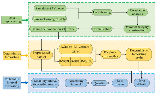
Figure 1.
The flowchart of the PV power forecasting.
- Data preprocessing. First, the raw PV power output data and meteorological data are cleaned. Next, the meteorological features are selected by calculating the Spearman correlation coefficient of the data. Then, the K-means clustering algorithm is employed to construct weather categories. After that, the data are normalized. Finally, the data are divided into training, validation, and test sets. Subsequently, the preprocessed dataset used for forecasting is obtained.
- Deterministic forecasting. Based on the XGBoost, RF, CatBoost, and LSTM models, the TLEL model is constructed. At the same time, the FRD approach is introduced to construct the R-XGBL, R-RFL, and R-CatBL models. The above models are combined using the reciprocal error method to construct the FRD-TLEL model, and then deterministic forecasting results are obtained.
- Probability interval forecasting. Based on the deterministic forecasting error dataset and preprocessed dataset, after selecting the loss function and quantile, the quantile forecasting results are obtained, and the forecasting interval is constructed to acquire the PV power interval forecasting results based on QR.
2.2. Data Description
The data used in this study were obtained from the Desert Knowledge Australia Solar Center (DKASC) in Alice Springs, Australia [38] (https://dkasolarcentre.com.au/source/alice-springs/yulara-total-of-all-yulara-sites-1, accessed on 19 September 2023). The PV array rated power is 263.0 kWp. The downloaded data included PV power output (kW), solar irradiance (W/m2), ambient temperature (°C), relative humidity (%rh), wind speed (m/s), wind direction (°), daily average precipitation (mm), etc. We selected the PV power output, solar irradiance, ambient temperature, relative humidity, and wind speed data with a time step of 5 min from 0:00 to 11:55 every day, from the 1 April 2016 to the 31 March 2018, from the downloaded data as the raw data for this study. The three criterion was utilized to detect outliers in the data; for large amounts of missing data within the forecasting period, all the data within that date were deleted, and, for cases of scattered missing data, the pre- and post-data filling interpolation method was used for processing [39]. In order to improve the forecasting accuracy and adapt to the forecasting model, by analyzing the non-zero range of daily effective PV power in different seasons, the daily forecasting time period from 7:00 to 18:00 was finally selected, and the time step of the data was adjusted from 5 min to 15 min. Thus, 31,725 sets of valid data containing 45 sample points per day were constructed for the correlation analysis and weather category construction.
2.3. Correlation Analysis of Multiple Features
Five sets of characteristic variables from the historical data, including PV power output, solar irradiance, ambient temperature, relative humidity, and wind speed, were extracted. Through observation, it can be seen that these five sets of data are all continuous variables. Then, scatter plots were used to sequentially determine whether the PV power output and the other four sets of variables displayed a linear correlation, as shown in Figure 2.
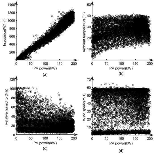
Figure 2.
Scatter plots of the PV power with solar irradiance, ambient temperature, relative humidity, and wind speed. (a) Solar irradiance; (b) ambient temperature; (c) relative humidity; and (d) wind speed.
From Figure 2, it can be seen that the correlation between the PV power and solar irradiance is linear, but the PV power is not linearly correlated with the ambient temperature, relative humidity, and wind speed. Therefore, the Spearman correlation coefficient method was selected to calculate the correlation [39]. The formula used is as follows:
where is the Spearman correlation coefficient; n is the number of samples; and are the positional value of certain meteorological factor and the PV power, respectively, and and are the average positional value of certain meteorological factor and the PV power. The thermal diagram of the Spearman correlation coefficient between the PV power and various meteorological features is shown in Figure 3.
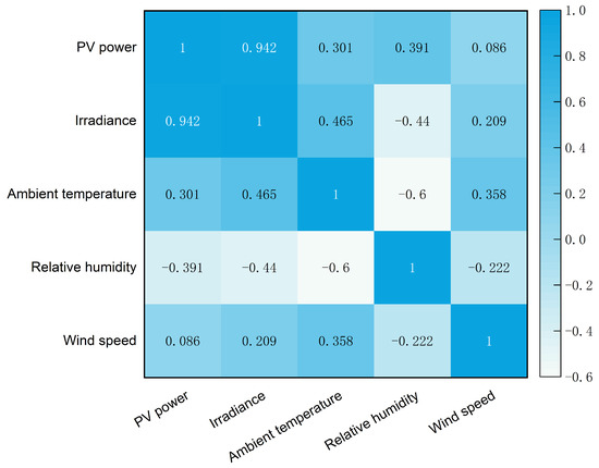
Figure 3.
Thermal diagram of the Spearman correlation coefficient between the PV power and various meteorological factors.
As shown in Figure 3, the PV power is highly positively correlated with the solar irradiance, positively correlated with the environmental temperature, negatively correlated with the relative humidity, and almost unrelated to the wind speed. Therefore, solar irradiance, environmental temperature, and relative humidity were selected as the initial input features of the model in this paper.
2.4. Weather Category Construction
Due to the lack of direct indication of weather types in the historical data, the K-means algorithm was used to classify weather types. The K-means algorithm is an iterative clustering analysis algorithm whose main function is to automatically classify similar samples into corresponding categories. Compared to other classification algorithms, the K-means clustering algorithm is simpler and very effective. It can cluster sample data without prior knowledge of any sample conditions, and the reasonable determination of the k values and initial cluster center points has a significant impact on the clustering effect [40,41].
Assuming that the given dataset A contains n objects, i.e., , where each object has features of m dimensions, we firstly initialized the k cluster centers and then calculated the Euclidean distance between each object and each cluster center. The calculation formula is as follows:
where represents the i-th object; represents the j-th cluster center; represents the t-th feature of the i-th object, and represents the t-th feature of the j-th clustering center.
The distance from each object to each cluster center was compared in sequence, and the object to the nearest cluster center was assigned; then, the k clusters were obtained. The center of the cluster was the mean of all the objects within the cluster in each feature, as shown in Equation (3), as follows:
where represents the j-th cluster, and represents the number of objects in the j-th cluster.
Based on the data of ambient temperature, relative humidity, and solar irradiance, the maximum, minimum, and average values of the above parameters on a single day were calculated as the input parameters for K-means clustering. The initial value of k was set to three. The clustering results of different seasons were obtained. The clustering centers in spring are shown in Table 1.

Table 1.
Clustering centers in spring.
As shown in Table 1, for the clustering center of cluster 3, both the average ambient temperature and the average solar irradiance are the maximum, while the average relative humidity is the minimum; for the clustering center of cluster 2, both the average ambient temperature and the solar irradiance are the minimum, while the average relative humidity is the maximum; and, for the clustering center of cluster 1, the average values of each feature are in the middle. Therefore, cluster 1 belongs to the category of cloudy days; cluster 2 belongs to the category of rainy days, and cluster 3 belongs to the category of sunny days. Similarly, we clustered the meteorological data for each season separately to obtain the number of different weather types for each season, as shown in Table 2.
Table 2.
Number of different weather types in each season.
As seen in Table 2, the number of rainy days is relatively small. To simplify the forecasting and improve the accuracy of the model forecasting, the two weather types of cloudy and rainy days were merged as cloudy or rainy days.
2.5. Construction of the TLEL Model
2.5.1. Ensemble Learning
EL is a method of constructing and combining multiple single learners to complete learning tasks. Firstly, multiple single weak learners were trained based on boosting or bagging learning methods, and then learning strategies such as averaging and voting were used to combine single weak learners to form a strong learner. The strong learners formed through EL had more significant generalization performance than the single learners [23,42].
The single learner algorithms used in this paper included the XGBoost algorithm, the RF algorithm, and the CatBoost algorithm.
2.5.2. XGBoost Algorithm
The XGBoost algorithm is an efficient gradient boosting decision tree (GBDT) algorithm, which is improved from the GBDT. As a forward addition model, it is one of the typical models of boosting methods. This algorithm iteratively generates a new tree by fitting residuals, forming a classifier with a higher accuracy and a stronger generalization ability. The basic regression tree model used in the XGBoost model is represented as follows [43]:
where K is the number of the trees; fk is a function in the function space R; is the forecasting value of the regression tree; xi is the i-th data input, and R is the set of all possible regression tree models.
The objective function of the XGBoost model is shown in Equation (5) as follows:
where is the difference between the forecasting value of the model and the actual value, and is the regular term of the scalar function.
The regularization penalty function was used to prevent overfitting of the model, as shown in Equation (6) [11], as follows:
where T is the number of leaf nodes; is the penalty function coefficient; is the score of the leaf node, and is the regularization penalty coefficient.
2.5.3. RF Algorithm
The RF algorithm is an algorithm that integrates multiple trees through EL. Its basic unit is the decision tree, which is one of the typical models of bagging methods. It can run effectively on large datasets and achieve good results for default value problems [11].
When constructing a decision tree, the RF algorithm uses the method of randomly selecting a split attribute set. Assuming the number of sample attributes is M, the specific process of the RF algorithm is as follows [44]:
- 1.
- Use the bootstrap method to repeatedly sample and randomly generate T training sets .
- 2.
- Use each training set to generate a corresponding decision tree. Before selecting attributes on each non-leaf node, randomly select m attributes from the M attributes as the splitting attribute set for the current node, and split the node in the best splitting method among these m attributes.
- 3.
- Each tree grows well, so there is no need for pruning.
- 4.
- For the test set sample B, use each decision tree to test it and obtain the corresponding category .
- 5.
- Using the voting method, select the category with the highest output from T decision trees as the category to which sample B belongs.
2.5.4. CatBoost Algorithm
The CatBoost algorithm is a gradient-lifting algorithm based on a decision tree improvement. Unlike traditional neural networks, it does not require a large number of samples as a training set and can perform high-accuracy forecasting based on small-scale samples. The CatBoost algorithm is one of the typical models of boosting class methods. The CatBoost algorithm can solve the problem of overfitting in traditional GBDT algorithms. It reduces the impact of gradient estimation bias through unbiased gradient estimation, thereby improving the model’s generalization ability [45].
In the traditional GBDT algorithm, the node splitting criterion is the label average value, while the CatBoost algorithm incorporates prior terms and weight coefficients to reduce the impact of noise and low-frequency category data on data distribution, as presented in Equation (7), as follows:
where is the feature of the i-th category of the k-th training sample; is the average value of all ; is the label of the j-th sample; I is the indicator function; p is the added prior term, and is the weight coefficient.
2.5.5. LSTM Algorithm
The LSTM neural network is a temporal RNN that can solve the long-term dependency problem that exists in general RNNs. The LSTM neural network is composed of three parts: an input gate, an output gate, and a forget gate. The structural diagram is shown in Figure 4 [20,46].
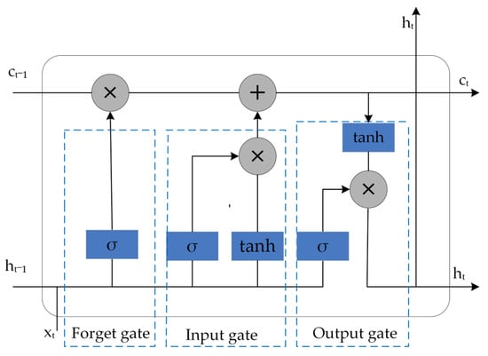
Figure 4.
The structure of the LSTM neural network.
The calculation formula for the information inside the LSTM cell is as follows [47]:
where xt is the input information at time t; and are the output information at time t and t − 1, respectively; and represent the cell states at time t and t − 1; and are the weight coefficients and deviations for each gate, respectively; and represent the activation function and hyperbolic tangent activation function, respectively, and ft, it, and ot are the state operation results of the forget gate, input gate, and output gate, respectively.
The input gate was used to control how much new information was added to the cell state at each time t; that is, xt and were processed using the and functions, respectively, to jointly determine what information was stored in the memory cell state. The forget gate determined the proportion of cell state information that needed to be retained in the current cell state at time t − 1. Moreover, the forget gate read the information of ht−1 and xt, and, if ft was zero, all the information of ct−1 was discarded, and, if ft was one, all the information of ct−1 was retained. The output gate determined the degree to which the ct was saved to the cell output at time t.
2.5.6. TLEL Model
Considering the limitations of a single learner, this paper constructed the TLEL model based on EL using single learners’ XGBoost, RF, CatBoost, and LSTM models.
In the first layer of the TLEL model, the dataset including the solar irradiance, environmental temperature, and relative humidity that had been classified by weather categories and normalized was used as the input to perform hyperparameter optimization on the single learners’ XGBoost, RF, and CatBoost models. Then, the forecasting results of each model were combined as a subsequent forecasting dataset.
In the second layer of the TLEL model, the subsequent forecasting dataset obtained through the first layer was utilized as the input to perform hyperparameter optimization on the meta-learner LSTM model, and the forecasting results of the TLEL model were obtained. The forecasting result set is denoted as and the error dataset is denoted as .
2.6. Construction of the Proposed FRD-TLEL Model
2.6.1. Feature Engineering
Feature engineering is the process of transforming raw data into features that better express the essence of a problem—that is, discovering features that have a significant impact on the dependent variable to improve model performance [48,49]. The implementation methods include feature dimensionality reduction and the FRD approaches.
In this paper, in addition to using the Spearman correlation coefficient to calculate the correlation for feature dimensionality reduction, the use of the FRD approach for machine learning is proposed, which trains the machine learning model by inputting a small number of influence features to obtain training results containing the model’s features as new gain features for further training of the model. This method can not only preserve the value of the original features in the dataset but also achieve a deep fusion between various models to improve model performance. This method can obtain data features through single-layer machine learning, with a high efficiency in feature acquisition and full-carrying information.
2.6.2. FRD-TLEL Model
The FRD-TLEL model was proposed in this paper, the framework of which is shown in Figure 5. Firstly, the XGBoost, RF, and CatBoost models were trained separately using the preprocessed meteorological feature dataset under the corresponding weather category as the input. Subsequently, the forecasting results of the three single models in the subsequent forecasting dataset were regarded as new gain features with corresponding model features, including the FRD data based on the XGBoost, RF, and CatBoost models, respectively. Secondly, the hyperparameters were optimized for the corresponding LSTM model based on the new gain features and preprocessed meteorological feature dataset, under corresponding weather categories. Then, the R-XGBL model, R-RFL model, and R-CatBL model were constructed. By constructing the R-XGBL model, the forecasting result set and error set were obtained. By constructing the R-RFL model, the forecasting result set and error set were obtained. By constructing the R-CatBL model, the forecasting result set and error set were obtained. Finally, the forecasting results of the TLEL, R-XGBL, R-RFL, and R-CatBL models were weighted and combined using the reciprocal error method to obtain the total forecasting results and errors .
where is the weight coefficient of the model; , , , and are the corresponding error values of , , , and sorted from small to large, respectively; is the forecasting result set corresponding to ; is the forecasting result set corresponding to ; is the forecasting result set corresponding to ; is the forecasting result set corresponding to , and is the actual PV power. From Equations (13)–(18), it can be seen that the reciprocal error method can amplify the advantages of small error models and reduce the disadvantages of large error models, thereby reducing the overall error of the combined model and achieving the goal of improving forecasting accuracy.
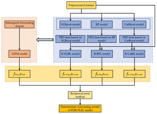
Figure 5.
Framework of the FRD-TLEL model.
2.7. Probability Interval Forecasting Model Based on QR
The QR model can make up for the shortcomings of ordinary linear regression models. Compared to traditional least squares regression models, QR can better solve the problem of dispersed or asymmetric distribution of explanatory variables when the shape of the conditional distribution is unknown. It can meet the requirements of exploring the global distribution of response variables while studying the expected mean of response variables, and it can comprehensively describe the possible range of dependent variables.
QR estimation is performed using the weighted minimum absolute deviation sum method, which can ignore the influence of outliers. Its results are more stable, which can be used to describe the global features of response variables and, thus, mine richer information. The specific representation of the QR model is as follows [37,50]:
where X is a vector of P-dimensional covariates; Y is a real value response variable; is an unknown univariate connection function; is a known function; is the given quantile, in the range of 0–1; is an index coefficient, and is a transposition of .
For the recognizability of the model, we assume that satisfies and that the first component is positive. The expression for is as follows:
The loss function is shown in Equation (21) as follows:
Assuming that is an independent and identically distributed sample from Equation (19), an estimate of can be obtained using the local linear method, represented as follows:
where , is a kernel function, and h is the bandwidth.
In this study, the steps for probability interval forecasting based on QR were as follows:
(1) Construction of interval forecasting models. Using the preprocessed dataset and the FRD-TLEL model-based short-term PV power deterministic forecasting error as the inputs, a loss function was set, and a QR interval forecasting model considering deterministic forecasting error was constructed.
(2) Forecasting of quantiles. In this step, we constructed a quantile forecasting matrix, selected quantiles, and performed quantile forecasting on PV power data based on the interval forecasting model established in step (1) to obtain forecasting results at different quantiles.
(3) The construction of forecasting intervals. The quantiles were selected to construct the upper and lower bounds of the PV power forecasting interval, and, thereby, the forecasting intervals were generated at different confidence levels.
2.8. Performance Metrics
In this paper, for deterministic forecasting, two performance evaluation metrics, including the mean absolute percentage error (MAPE) and the root mean square error (RMSE) [21,51], were employed to evaluate the forecasting results. The MAPE is a measure of relative error that uses absolute values to avoid the cancellation of positive and negative errors. A smaller MAPE value indicates better model quality and more accurate forecasting. The RMSE is the arithmetic square root of the mean square error, reflecting the degree of deviation between the true value and the forecasting value. The smaller the RMSE value, the better the quality of the model and the more accurate the forecasting. These two performance metrics used for deterministic forecasting models can be expressed by Equations (23) and (24) as follows:
where is the forecasting value of the model, and is the actual value of PV power.
In this paper, for probabilistic interval forecasting, the performance metrics consisted of the prediction interval coverage percentage (PICP) and of the prediction interval normalized average width (PINAW) [52,53], which are indicated as follows:
where is a Boolean value. If the actual power value is within the range, the value of is one, otherwise it is zero. is the bandwidth of the i-th interval.
The PICP is used to evaluate the accuracy of the forecasting interval. The larger the PICP value, the higher the accuracy of the model’s forecasting. The PINAW is employed to evaluate the width of the interval. The smaller the PINAW value, the narrower the upper and lower boundary range of the model’s forecasting.
3. Forecasting Results and Discussion
In this section, the preprocessed dataset that underwent data cleaning, correlation analysis, weather category construction, normalization, and classification of training, validation, and test sets is used by the proposed FRD-TLEL model for deterministic forecasting. The forecasting results of the proposed model under different seasons and weather types are compared with those of other models. Then, we perform probability interval forecasting and compare the interval forecasting results under different confidence levels, seasons, and weather types. The detailed findings and discussions are provided below.
3.1. Analysis of Deterministic Forecasting Results
The data used for training, validation, and testing the model covers the period from the 1 April 2016 to the 31 March 2018. This dataset includes the meteorological data (solar irradiance, ambient temperature, and relative humidity) and the PV power data collected every day from 7:00 to 18:00, with a time step of 15 min. Among these data, eight specific days were chosen as the forecasted days: the 18 November 2017 (the sunny day in spring), the 22 October 2017 (the cloudy or rainy in spring), the 26 February 2017 (the sunny day in summer), the 21 December 2017 (the cloudy or rainy in summer), the 30 March 2017 (the sunny day in autumn), the 5 May 2017 (the cloudy or rainy in autumn), the 30 August 2017 (the sunny day in winter), and the 25 July 2017 (the cloudy or rainy in winter). The data of these eight days were used as the test dataset. The remaining data were divided into training and validation sets for the training models and the K-fold cross-validation. To verify the performance of the FRD-TLEL model proposed in this paper, the forecasting results of this model are compared with the BP, XGBoost, RF, CatBoost, LSTM, R-XGBL, R-RFL, R-CatBL, and TLEL models.
Figure 6 shows the comparison between the deterministic forecasting results of the BP, XGBoost, RF, CatBoost, LSTM, R-XGBL, R-RFL, R-CatBL, TLEL and FRD-TLEL models and the actual PV power under sunny weather in each season.
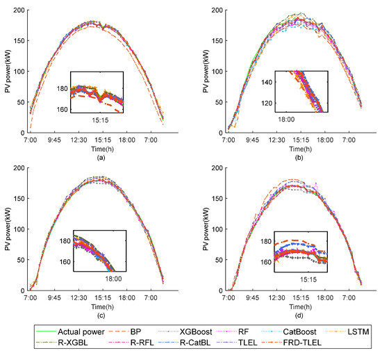
Figure 6.
Comparison of forecasting results of various models on sunny days in different seasons. (a) Spring; (b) summer; (c) autumn; and (d) winter.
From Figure 6 and Figure 7, it can be seen that the shapes of the PV power curves on sunny days in each season all rise at first and then fall, and the overall distribution is smooth, with occasional slight fluctuations. The forecasting curves of the FRD-TLEL model are closer to the actual values compared to other models. On cloudy or rainy days in each season, the PV power curves are distributed in a large fluctuation curve. The forecasting curves of different weather types in different seasons reflect the fact that the deterministic forecasting results of the FRD-TLEL model are closer to the actual value than those of other models. Furthermore, the forecasting curves of the TLEL model are closer to the actual values than each one of the single models in different seasons and in different weather types. These two figures indicate that the proposed model is more effective in forecasting PV power and reducing forecasting errors.
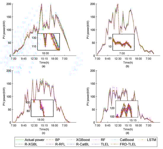
Figure 7.
Comparison of forecasting results of various models on cloudy or rainy days in different seasons. (a) Spring; (b) summer; (c) autumn; and (d) winter.
The error comparison of different forecasting methods on the sunny days in different seasons is shown in Table 3, and the error comparison of different forecasting methods on the cloudy or rainy days in different seasons is presented in Table 4. The error comparison of different forecasting methods on all the forecasted days is listed in Table 5. The decrease in the performance metrics of the FRD-TLEL model compared to the other nine models on sunny days under different seasons is shown in Figure 8. The decrease in the performance metrics of the FRD-TLEL model compared to the other nine models on cloudy or rainy days in different seasons is shown in Figure 9.
Table 3.
The error comparison of different forecasting methods on sunny days in different seasons.
Table 4.
The error comparison of different forecasting methods on cloudy or rainy days in different seasons.
Table 5.
The error comparison of different forecasting methods on all forecasted days.
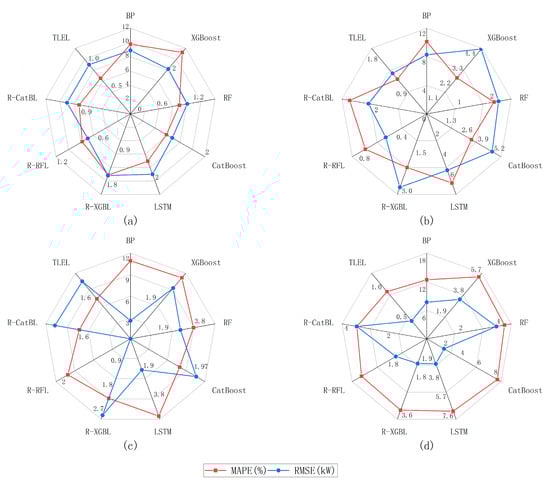
Figure 8.
The decrease in the performance metrics of the FRD-TLEL model compared to other models on sunny days in different seasons and with different weather types. (a) Spring; (b) summer; (c) autumn; and (d) winter.
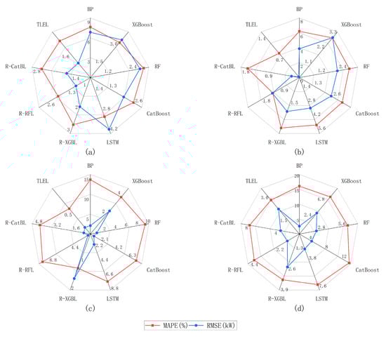
Figure 9.
The decrease in the performance metrics of the FRD-TLEL model compared to other models on cloudy or rainy days in different seasons and with different weather types. (a) Spring; (b) summer; (c) autumn; and (d) winter.
Taking the sunny day in spring in Table 3 and Figure 8 as an example, it can be seen that, in a comparison with the BP, XGBoost, RF, CatBoost, LSTM, R-XGBL, R-RFL, R-CatBL, and TLEL models, the MAPE of the FRD-TLEL model decreased by 9.76%, 3%, 0.91%, 1.07%, 1.51%, 1.6%, 0.82%, 0.85%, and 0.75%, respectively; the RMSE decreased by 8.9 kW, 2.19 kW, 1.04 kW, 1.21 kW, 1.9 kW, 1.61 kW, 0.74 kW, 1.05 kW, and 1 kW, respectively. Furthermore, compared to the single models BP, XGBoost, RF, CatBoost, and LSTM, the MAPE of the TLEL model is reduced by 9.01%, 2.25%, 0.16%, 0.32%, and 0.76%, respectively, and the RMSE is reduced by 7.9 kW, 1.19 kW, 0.04 kW, 0.21 kW, and 0.9 kW, respectively. The forecasting results demonstrate that the FRD-TLEL model has the lowest forecasting error and that the TLEL has a lower forecasting error than the single models on the sunny day in spring.
On the rainy day in spring, in comparison with the BP, XGBoost, RF, CatBoost, LSTM, R-XGBL, R-RFL, R-CatBL, and TLEL models, the MAPE of the FRD-TLEL model decreased by 7.64%, 3.09%, 2.75%, 2.48%, 3.12%, 2.6%, 2.61%, 2.45%, and 2.41%, respectively, while the RMSE decreased by 6.85 kW, 3.32 kW, 2.58 kW, 1.99 kW, 4 kW, 1.81 kW, 1.5 kW, 1.55 kW, and 0.96 kW, respectively. Furthermore, compared to the BP, XGBoost, RF, CatBoost, and LSTM models, the MAPE of the TLEL model is reduced by 5.23%, 0.68%, 0.34%, 0.07%, and 0.71%, respectively, and the RMSE is reduced by 5.89 kW, 2.36 kW, 1.62 kW, 1.03 kW, and 3.04 kW, respectively. The forecasting results demonstrate that the FRD-TLEL model has the lowest forecasting error and that the TLEL model has a lower forecasting error than the single models on the cloudy or rainy day in spring. It is worth mentioning that, compared to sunny weather, the proposed model has a greater reduction in forecasting error compared to other models, indicating that the proposed forecasting method not only has a high forecasting accuracy but is also stable.
As shown in Table 3, Table 4 and Table 5 and Figure 8 and Figure 9, compared to the BP, XGBoost, RF, CatBoost, LSTM, R-XGBL, R-RFL, R-CatBL, and TLEL models, no matter the season or weather type, the FRD-TLEL model has the lowest MAPE and RMSE and has the best forecasting performance. It has a significant advantage in sunny weather. In cloudy or rainy weather, due to the significant fluctuations of the meteorological factors, the stability of PV power is reduced, and its forecasting accuracy is slightly lower than that of sunny weather, but the error reduction in the FRD-TLEL model is more significant compared to sunny weather. Compared to the single models, the TLEL model also has a similar rule. This indicates that the proposed forecasting method can effectively improve forecasting accuracy under different weather types.
To further demonstrate the superiority of the proposed forecasting method, the forecasting results of the FRD-TLEL model are compared with other studies. Firstly, they are compared in terms of their forecasting accuracy. In the forecasting results of winter data in [20], the MAPE values for two sunny days are 2.5% and 1.5%, respectively, and the MAPE values for two cloudy days are 15.3% and 10.1%, respectively; the MAPE values for two rainy days are 13.3% and 22.1%, respectively. However, in the forecasting results of the FRD-TLEL model in this paper, the MAPE for sunny weather is 1.03%, while the MAPE for cloudy or rainy days is 3.26%, with lower errors than the CD-NARX-LSTM LightGBM model in [20]. For [31], in the annual forecast results, the MAPE values for sunny, cloudy, and rainy days are 6.52%, 6.69%, and 7.07%, respectively. However, in this paper, regardless of the weather type in spring, summer, autumn, and winter, the MAPE value is lower than the WVCFM model in [31]. Through comparison, it is proven that the model proposed in this paper has a higher forecasting accuracy. Secondly, the forecasting time is compared. In [20], the average run time of the NARX-LSTM-LightGBM model is 45.23 min, and the average run time of the CD-NARX-LSTM-LightGBM model is 67.59 min. Meanwhile, in this paper, through multiple experiments, the average running time of different types of forecasting models is shown in Table 6, proving that the proposed forecasting method has a higher forecasting efficiency.
Table 6.
The average running time of different types of forecasting models (formatted in minutes.seconds.milliseconds).
In summary, the short-term PV power deterministic forecasting method proposed in this paper greatly improves forecasting accuracy and efficiency.
3.2. Analysis of Probability Interval Forecasting Results
By combining the deterministic forecasting results of the FRD-TLEL model with the QR estimation, interval forecasting of PV power is performed for different seasons and weather types. The interval forecasting curves of PV power under 95%, 75%, and 50% confidence levels are obtained for sunny weather and cloudy or rainy weather in each season, as shown in Figure 10, Figure 11 and Figure 12. The interval forecasting performance metrics for different seasons and weather types at different confidence levels are shown in Table 7.
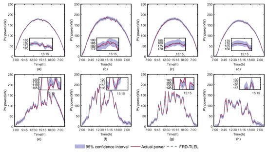
Figure 10.
Forecasting intervals for different seasons and weather types at a 95% confidence level. (a) Sunny day in spring; (b) sunny day in summer; (c) sunny day in autumn; (d) sunny day in winter; (e) cloudy or rainy day in spring; (f) cloudy or rainy day in summer; (g) cloudy or rainy day in autumn; and (h) cloudy or rainy day in winter.
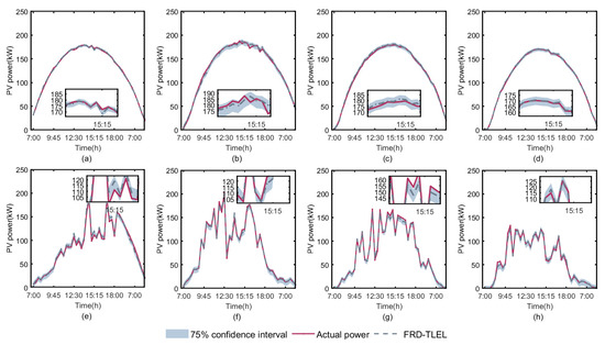
Figure 11.
Forecasting intervals for different seasons and weather types at a 75% confidence level. (a) Sunny day in spring; (b) sunny day in summer; (c) sunny day in autumn; (d) sunny day in winter; (e) cloudy or rainy day in spring; (f) cloudy or rainy day in summer; (g) cloudy or rainy day in autumn; and (h) cloudy or rainy day in winter.
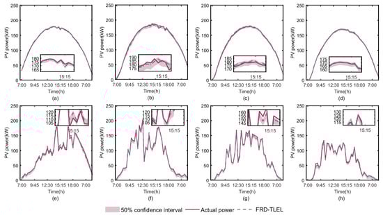
Figure 12.
Forecasting intervals for different seasons and weather types at a 50% confidence level. (a) Sunny day in spring; (b) sunny day in summer; (c) sunny day in autumn; (d) sunny day in winter; (e) cloudy or rainy day in spring; (f) cloudy or rainy day in summer; (g) cloudy or rainy day in autumn; and (h) cloudy or rainy day in winter.
Table 7.
Interval forecasting performance metrics for different seasons and weather types at different confidence levels.
According to Figure 10, Figure 11 and Figure 12 and Table 7, it is clear that the PICP levels for each season and weather type at 95%, 75%, and 50% confidence levels are higher than their basic confidence level, meeting the confidence conditions for interval forecasting. The PICP and PINAW of interval forecasting results for each season and weather type decrease with the decrease in confidence level. At a 95% confidence level, the interval PINAW is the largest and PICP is the highest, while, at a 50% confidence level, the interval PINAW is the narrowest and PICP is the lowest. It can be seen that the probability forecasting model based on QR proposed in this paper can achieve satisfactory forecasting in different seasons, weather types, and confidence levels.
In summary, in order to verify the superiority of the proposed forecasting method, different models were constructed based on data clustering, and deterministic and probability forecasting were performed separately. The deterministic forecasting results indicate that the FRD-TLEL model has a higher forecasting accuracy than the other models in different seasons and weather types. The probability forecasting results indicate that the proposed model has a good forecasting interval and reduces the uncertainty of PV power generation. The forecasting method proposed in this paper can effectively improve the accuracy of short-term PV power forecasting. When applied in practice, it can improve the utilization rate of renewable energy, promote sustainable development, and help dispatch departments to better plan and optimize the real-time operation of the power system, ensuring the safe and stable operation of the power system after a high proportion of grid-connected PV power generation is achieved.
4. Conclusions
The goal of this study is to propose a short-term PV power forecasting method using K-means clustering, EL, the FRD approach, and QR to improve the accuracy of deterministic and probabilistic forecasting of PV power, thereby promoting the safe and stable operation of the power grid and enhancing the sustainable utilization of renewable energy. The main conclusions are as follows:
- The proposed FRD-TLEL model was effective in increasing the accuracy of forecasting as compared to the single models, providing three apparent advantages. Firstly, constructing the TLEL model through EL avoids the limitations of a single forecasting model. Secondly, by inputting a small number of influential features to train each single model, the training results containing the model features are obtained, thus forming new gain features for the further training of the models. This FRD approach can preserve the value of the original features in the dataset and achieve a deep fusion between various models to improve model forecasting accuracy. Furthermore, when large errors occur in individual models, the combination of forecasting models with the reciprocal error method can largely reduce the impact of said errors on the accuracy of the forecasting models.
- The results of the deterministic forecasting experiments indicate that the proposed FRD-TLEL model has the highest forecasting accuracy compared to the other models. Compared to the BP, XGBoost, RF, CatBoost, LSTM, R-XGBL, R-RFL, R-CatBL, and TLEL models, the FRD-TLEL model has the lowest MAPE and RMSE on sunny and cloudy or rainy days in spring, summer, autumn, and winter. On the sunny day in winter, the MAPE values of other models are 13.46%, 6.69%, 5.17%, 9.49%, 8.23%, 4.5%, 4.01%, 4.33%, and 2.02%, respectively, while the lowest MAPE of the FRD-TLEL model is 1.03%; the RMSE values of the other models are 8.78 kW, 4.64 kW, 4.75 kW, 3.12 kW, 3.53 kW, 2.31 kW, 2.46 kW, 4.34 kW, 1.54 kW, and 1.04 kW, respectively, while the RMSE of the FRD-TLEL model is lowest at 1.04 kW. Compared to models in some other studies, the FRD-TLEL model also has a higher forecasting accuracy.
- The experimental results of probability forecasting show that the FRD-TLEL model based on QR has a good forecasting performance for different seasons and weather conditions at the 95%, 75%, and 50% confidence levels.
The high forecasting accuracy of the model proposed in this paper has only been validated in the deterministic and probabilistic forecasting of short-term PV power. Exploring models with high forecasting accuracy and efficiency at different time scales is one of future research directions.
Author Contributions
Conceptualization, H.W. and J.W.; methodology, H.W. and S.Y.; software, H.W. and S.Y.; validation, S.Y. and D.J.; formal analysis, S.Y. and N.M.; investigation, J.F.; resources, S.W.; data curation, H.L.; writing—original draft preparation, H.W. and S.Y.; writing—review and editing, H.W. and J.W.; visualization, T.Z.; supervision, Y.X.; project administration, D.J.; funding acquisition, J.W. and H.W. All authors have read and agreed to the published version of the manuscript.
Funding
This research was supported by the Liaoning Province Scientific Research Funding Program, grant number LJKZ0681, and by the Science and Technology Project in Electric Power Research Institute of State Grid Liaoning Electric Power Supply Co., Ltd., grant number 2022YF-83.
Institutional Review Board Statement
Not applicable.
Informed Consent Statement
Not applicable.
Data Availability Statement
Not applicable.
Acknowledgments
We thank the editors and reviewers for their helpful suggestions.
Conflicts of Interest
The authors declare no conflict of interest.
Nomenclature
| PV | Photovoltaic | XGBoost | eXtreme Gradient Boosting algorithm |
| AI | Artificial intelligence | R-XGBL | FRD-XGBoost-LSTM |
| BP | Back propagation | R-RFL | FRD-RF-LSTM |
| SVM | Support vector machine | R-CatBL | FRD-CatBoost-LSTM |
| ANN | Artificial neural network | QR | Quantile regression |
| RF | Random forest | WOA | White optimization algorithm |
| DL | Deep learning | LSSVM | Least squares support vector machine model |
| CNN | Convolutional neural network | ELM | Extreme learning machine |
| RNN | Recurrent neural network | GRU | Gated recursive unit |
| LSTM | Long short-term memory | KDE | Kernel density estimation |
| EL | Ensemble learning | MAPE | Mean absolute percentage error |
| FRD | Feature rise-dimensional | RMSE | Root mean square error |
| TLEL | Two-layer ensemble learning | PICP | Prediction interval coverage percentage |
| FRD-TLEL | Feature rise-dimensional two-layer ensemble learning | PINAW | Prediction interval normalized average width |
| Spearman correlation coefficient | Deviations for each gate | ||
| n | Number of samples | Activation function | |
| Positional value of certain meteorological factor | Hyperbolic tangent activation function | ||
| Positional value of PV power | ft | State operation results of the forget gate | |
| Average positional value of certain meteorological factor | it | State operation results of the input gate | |
| Average positional value of PV power | ot | State operation results of the output gate | |
| A | Given dataset | Weight coefficient of the model | |
| The i-th object | Error value of TLEL model | ||
| The t-th feature of the i-th object | Error value of R-XGBL model | ||
| the j-th cluster center | Error value of R-RFL model | ||
| The t-th feature of the j-th clustering center | Error value of R-CatBL model | ||
| The j-th cluster | The maximum value of , , , and | ||
| Number of objects in the j-th cluster | The second maximum of , , , and | ||
| K | Number of the trees | The third maximum of , , , and | |
| fk | A function in the function space R | The minimum value of , , , and | |
| Forecasting value of the regression tree | Forecasting result set corresponding to | ||
| xi | The i-th data input | Forecasting result set corresponding to | |
| R | Set of all possible regression tree models | Forecasting result set corresponding to | |
| Difference between the forecasting value of the model and the actual value | Forecasting result set corresponding to | ||
| Regular term of the scalar function | Actual PV power | ||
| T | Number of leaf nodes | Forecasting result | |
| Penalty function coefficient | X | A vector of P-dimensional covariates | |
| Score of the leaf node | Y | Real value response variable | |
| Regularization penalty coefficient | An unknown univariate connection function | ||
| Feature of the i-th category of the k-th training sample | Known function | ||
| The average value of all | Given quantile | ||
| Label of the j-th sample | Index coefficient | ||
| I | Indicator function | Transposition of | |
| p | Added prior term | Kernel function | |
| Weight coefficient | h | Bandwidth | |
| xt | Input information at time t | Forecasting value | |
| Output information at time t | Actual value of PV power | ||
| Cell states at time t | Boolean value | ||
| Weight coefficients for each gate | Bandwidth of the i-th interval |
References
- Liu, Z.-F.; Li, L.-L.; Liu, Y.-W.; Liu, J.-Q.; Li, H.-Y.; Shen, Q. Dynamic Economic Emission Dispatch Considering Renewable Energy Generation: A Novel Multi-Objective Optimization Approach. Energy 2021, 235, 121407. [Google Scholar] [CrossRef]
- Soni, J.; Bhattacharjee, K. Multi-Objective Dynamic Economic Emission Dispatch Integration with Renewable Energy Sources and Plug-in Electrical Vehicle Using Equilibrium Optimizer. Environ. Dev. Sustain. 2023. [Google Scholar] [CrossRef]
- Acharya, S.; Ganesan, S.; Kumar, D.V.; Subramanian, S. Optimization of Cost and Emission for Dynamic Load Dispatch Problem with Hybrid Renewable Energy Sources. Soft Comput. 2023, 27, 14969–15001. [Google Scholar] [CrossRef]
- Zhang, J.; Liu, Z.; Chen, T. Interval Prediction of Ultra-Short-Term Photovoltaic Power Based on a Hybrid Model. Electr. Power Syst. Res. 2023, 216, 109035. [Google Scholar] [CrossRef]
- Zhou, W.; Jiang, H.; Chang, J. Forecasting Renewable Energy Generation Based on a Novel Dynamic Accumulation Grey Seasonal Model. Sustainability 2023, 15, 12188. [Google Scholar] [CrossRef]
- Das, U.K.; Tey, K.S.; Seyedmahmoudian, M.; Mekhilef, S.; Idris, M.Y.I.; Van Deventer, W.; Horan, B.; Stojcevski, A. Forecasting of Photovoltaic Power Generation and Model Optimization: A Review. Renew. Sustain. Energy Rev. 2018, 81, 912–928. [Google Scholar] [CrossRef]
- Han, S.; Qiao, Y.; Yan, J.; Liu, Y.; Li, L.; Wang, Z. Mid-to-Long Term Wind and Photovoltaic Power Generation Prediction Based on Copula Function and Long Short Term Memory Network. Appl. Energy 2019, 239, 181–191. [Google Scholar] [CrossRef]
- Tang, Y.; Yang, K.; Zhang, S.; Zhang, Z. Photovoltaic Power Forecasting: A Hybrid Deep Learning Model Incorporating Transfer Learning Strategy. Renew. Sustain. Energy Rev. 2022, 162, 112473. [Google Scholar] [CrossRef]
- Niu, D.; Wang, K.; Sun, L.; Wu, J.; Xu, X. Short-Term Photovoltaic Power Generation Forecasting Based on Random Forest Feature Selection and CEEMD: A Case Study. Appl. Soft Comput. 2020, 93, 106389. [Google Scholar] [CrossRef]
- Zhang, L.; He, Y.; Wu, H.; Yang, X.; Ding, M. Ultra-Short-Term Multi-Step Probability Interval Prediction of Photovoltaic Power: A Framework with Time-Series-Segment Feature Analysis. Sol. Energy 2023, 260, 71–82. [Google Scholar] [CrossRef]
- Dai, Y.; Wang, Y.; Leng, M.; Yang, X.; Zhou, Q. LOWESS Smoothing and Random Forest Based GRU Model: A Short-Term Photovoltaic Power Generation Forecasting Method. Energy 2022, 256, 124661. [Google Scholar] [CrossRef]
- Sobri, S.; Koohi-Kamali, S.; Rahim, N.A. Solar Photovoltaic Generation Forecasting Methods: A Review. Energy Convers. Manag. 2018, 156, 459–497. [Google Scholar] [CrossRef]
- Mayer, M.J.; Gróf, G. Extensive Comparison of Physical Models for Photovoltaic Power Forecasting. Appl. Energy 2021, 283, 116239. [Google Scholar] [CrossRef]
- Ahmed, R.; Sreeram, V.; Mishra, Y.; Arif, M.D. A Review and Evaluation of the State-of-the-Art in PV Solar Power Forecasting: Techniques and Optimization. Renew. Sustain. Energy Rev. 2020, 124, 109792. [Google Scholar] [CrossRef]
- Wang, Z.; Wang, Y.; Cao, S.; Fan, S.; Zhang, Y.; Liu, Y. A Robust Spatial-Temporal Prediction Model for Photovoltaic Power Generation Based on Deep Learning. Comput. Electr. Eng. 2023, 110, 108784. [Google Scholar] [CrossRef]
- Wang, H.; Wang, J.; Piao, Z. Photovoltaic Power Forecasting Based on Similar Time Considering Influence Factor of Bad Air Quality. Appl. Soft Comput. 2021, 102, 106957. [Google Scholar]
- Pan, M.; Li, C.; Gao, R.; Huang, Y.; You, H.; Gu, T.; Qin, F. Photovoltaic Power Forecasting Based on a Support Vector Machine with Improved Ant Colony Optimization. J. Clean. Prod. 2020, 277, 123948. [Google Scholar] [CrossRef]
- Scott, C.; Ahsan, M.; Albarbar, A. Machine Learning for Forecasting a Photovoltaic (PV) Generation System. Energy 2023, 278, 127807. [Google Scholar] [CrossRef]
- Abdellatif, A.; Mubarak, H.; Ahmad, S.; Ahmed, T.; Shafiullah, G.M.; Hammoudeh, A.; Abdellatef, H.; Rahman, M.M.; Gheni, H.M. Forecasting Photovoltaic Power Generation with a Stacking Ensemble Model. Sustainability 2022, 14, 11083. [Google Scholar] [CrossRef]
- Gao, H.; Qiu, S.; Fang, J.; Ma, N.; Wang, J.; Cheng, K.; Wang, H.; Zhu, Y.; Hu, D.; Liu, H.; et al. Short-Term Prediction of PV Power Based on Combined Modal Decomposition and NARX-LSTM-LightGBM. Sustainability 2023, 15, 8266. [Google Scholar] [CrossRef]
- Zhen, H.; Niu, D.; Wang, K.; Shi, Y.; Ji, Z.; Xu, X. Photovoltaic Power Forecasting Based on GA Improved Bi-LSTM in Microgrid without Meteorological Information. Energy 2021, 231, 120908. [Google Scholar] [CrossRef]
- Peng, T.; Fu, Y.; Wang, Y.; Xiong, J.; Suo, L.; Nazir, M.S.; Zhang, C. An Intelligent Hybrid Approach for Photovoltaic Power Forecasting Using Enhanced Chaos Game Optimization Algorithm and Locality Sensitive Hashing Based Informer Model. J. Build. Eng. 2023, 78, 107635. [Google Scholar] [CrossRef]
- Banik, R.; Biswas, A. Improving Solar PV Prediction Performance with RF-CatBoost Ensemble: A Robust and Complementary Approach. Renew. Energy Focus 2023, 46, 207–221. [Google Scholar] [CrossRef]
- Wang, F.; Xuan, Z.; Zhen, Z.; Li, K.; Wang, T.; Shi, M. A Day-Ahead PV Power Forecasting Method Based on LSTM-RNN Model and Time Correlation Modification under Partial Daily Pattern Prediction Framework. Energy Convers. Manag. 2020, 212, 112766. [Google Scholar] [CrossRef]
- Guo, X.; Gao, Y.; Zheng, D.; Ning, Y.; Zhao, Q. Study on Short-Term Photovoltaic Power Prediction Model Based on the Stacking Ensemble Learning. Energy Rep. 2020, 6, 1424–1431. [Google Scholar] [CrossRef]
- Wu, Y.-K.; Huang, C.-L.; Phan, Q.-T.; Li, Y.-Y. Completed Review of Various Solar Power Forecasting Techniques Considering Different Viewpoints. Energies 2022, 15, 3320. [Google Scholar] [CrossRef]
- Talaat, M.; Said, T.; Essa, M.A.; Hatata, A.Y. Integrated MFFNN-MVO Approach for PV Solar Power Forecasting Considering Thermal Effects and Environmental Conditions. Int. J. Electr. Power Energy Syst. 2022, 135, 107570. [Google Scholar] [CrossRef]
- Li, P.; Zhou, K.; Lu, X.; Yang, S. A Hybrid Deep Learning Model for Short-Term PV Power Forecasting. Appl. Energy 2020, 259, 114216. [Google Scholar] [CrossRef]
- Liu, Y.; Liu, Y.; Cai, H.; Zhang, J. An Innovative Short-Term Multihorizon Photovoltaic Power Output Forecasting Method Based on Variational Mode Decomposition and a Capsule Convolutional Neural Network. Appl. Energy 2023, 343, 121139. [Google Scholar] [CrossRef]
- Van Der Meer, D.W.; Widén, J.; Munkhammar, J. Review on Probabilistic Forecasting of Photovoltaic Power Production and Electricity Consumption. Renew. Sustain. Energy Rev. 2018, 81, 1484–1512. [Google Scholar] [CrossRef]
- Liu, L.; Zhao, Y.; Chang, D.; Xie, J.; Ma, Z.; Sun, Q.; Yin, H.; Wennersten, R. Prediction of Short-Term PV Power Output and Uncertainty Analysis. Appl. Energy 2018, 228, 700–711. [Google Scholar] [CrossRef]
- Li, K.; Wang, R.; Lei, H.; Zhang, T.; Liu, Y.; Zheng, X. Interval Prediction of Solar Power Using an Improved Bootstrap Method. Sol. Energy 2018, 159, 97–112. [Google Scholar] [CrossRef]
- Mitrentsis, G.; Lens, H. An Interpretable Probabilistic Model for Short-Term Solar Power Forecasting Using Natural Gradient Boosting. Appl. Energy 2022, 309, 118473. [Google Scholar] [CrossRef]
- Gu, B.; Shen, H.; Lei, X.; Hu, H.; Liu, X. Forecasting and Uncertainty Analysis of Day-Ahead Photovoltaic Power Using a Novel Forecasting Method. Appl. Energy 2021, 299, 117291. [Google Scholar] [CrossRef]
- Long, H.; Zhang, C.; Geng, R.; Wu, Z.; Gu, W. A Combination Interval Prediction Model Based on Biased Convex Cost Function and Auto-Encoder in Solar Power Prediction. IEEE Trans. Sustain. Energy 2021, 12, 1561–1570. [Google Scholar] [CrossRef]
- Pan, C.; Tan, J.; Feng, D. Prediction Intervals Estimation of Solar Generation Based on Gated Recurrent Unit and Kernel Density Estimation. Neurocomputing 2021, 453, 552–562. [Google Scholar] [CrossRef]
- Huang, Q.; Wei, S. Improved Quantile Convolutional Neural Network with Two-Stage Training for Daily-Ahead Probabilistic Forecasting of Photovoltaic Power. Energy Convers. Manag. 2020, 220, 113085. [Google Scholar] [CrossRef]
- dka Solar Center. 263.0kW, Total of All Sites. Available online: https://dkasolarcentre.com.au/source/alice-springs/yulara-total-of-all-yulara-sites-1 (accessed on 19 September 2023).
- Huang, C.; Yang, M. Memory Long and Short Term Time Series Network for Ultra-Short-Term Photovoltaic Power Forecasting. Energy 2023, 279, 127961. [Google Scholar] [CrossRef]
- Liu, D.; Sun, K. Random Forest Solar Power Forecast Based on Classification Optimization. Energy 2019, 187, 115940. [Google Scholar] [CrossRef]
- Zhen, Z.; Liu, J.; Zhang, Z.; Wang, F.; Chai, H.; Yu, Y.; Lu, X.; Wang, T.; Lin, Y. Deep Learning Based Surface Irradiance Mapping Model for Solar PV Power Forecasting Using Sky Image. IEEE Trans. Ind. Appl. 2020, 56, 3385–3396. [Google Scholar] [CrossRef]
- Khan, W.; Walker, S.; Zeiler, W. Improved Solar Photovoltaic Energy Generation Forecast Using Deep Learning-Based Ensemble Stacking Approach. Energy 2022, 240, 122812. [Google Scholar] [CrossRef]
- Zhou, B.; Chen, X.; Li, G.; Gu, P.; Huang, J.; Yang, B. XGBoost–SFS and Double Nested Stacking Ensemble Model for Photovoltaic Power Forecasting under Variable Weather Conditions. Sustainability 2023, 15, 13146. [Google Scholar] [CrossRef]
- Prasad, R.; Ali, M.; Kwan, P.; Khan, H. Designing a Multi-Stage Multivariate Empirical Mode Decomposition Coupled with Ant Colony Optimization and Random Forest Model to Forecast Monthly Solar Radiation. Appl. Energy 2019, 236, 778–792. [Google Scholar] [CrossRef]
- Prokhorenkova, L.; Gusev, G.; Vorobev, A.; Dorogush, A.V.; Gulin, A. CatBoost: Unbiased Boosting with Categorical Features. arXiv 2019, arXiv:1706.09516. [Google Scholar]
- Zhou, H.; Zhang, Y.; Yang, L.; Liu, Q.; Yan, K.; Du, Y. Short-Term Photovoltaic Power Forecasting Based on Long Short Term Memory Neural Network and Attention Mechanism. IEEE Access 2019, 7, 78063–78074. [Google Scholar] [CrossRef]
- Ospina, J.; Newaz, A.; Faruque, M.O. Forecasting of PV Plant Output Using Hybrid Wavelet-based LSTM-DNN Structure Model. IET Renew. Power Gener. 2019, 13, 1087–1095. [Google Scholar] [CrossRef]
- Pirhooshyaran, M.; Scheinberg, K.; Snyder, L.V. Feature Engineering and Forecasting via Derivative-Free Optimization and Ensemble of Sequence-to-Sequence Networks with Applications in Renewable Energy. Energy 2020, 196, 117136. [Google Scholar] [CrossRef]
- Salcedo-Sanz, S.; Cornejo-Bueno, L.; Prieto, L.; Paredes, D.; García-Herrera, R. Feature Selection in Machine Learning Prediction Systems for Renewable Energy Applications. Renew. Sustain. Energy Rev. 2018, 90, 728–741. [Google Scholar] [CrossRef]
- Hu, J.; Tang, J.; Lin, Y. A Novel Wind Power Probabilistic Forecasting Approach Based on Joint Quantile Regression and Multi-Objective Optimization. Renew. Energy 2020, 149, 141–164. [Google Scholar] [CrossRef]
- Ray, B.; Shah, R.; Islam, M.R.; Islam, S. A New Data Driven Long-Term Solar Yield Analysis Model of Photovoltaic Power Plants. IEEE Access 2020, 8, 136223–136233. [Google Scholar] [CrossRef]
- Yildiz, C.; Acikgoz, H.; Korkmaz, D.; Budak, U. An improved residual-based convolutional neural network for very short-term wind power forecasting. Energy Convers. Manag. 2021, 228, 113731. [Google Scholar] [CrossRef]
- An, Y.; Dang, K.; Shi, X.; Jia, R.; Zhang, K.; Huang, Q. A Probabilistic Ensemble Prediction Method for PV Power in the Nonstationary Period. Energies 2021, 14, 859. [Google Scholar] [CrossRef]
Disclaimer/Publisher’s Note: The statements, opinions and data contained in all publications are solely those of the individual author(s) and contributor(s) and not of MDPI and/or the editor(s). MDPI and/or the editor(s) disclaim responsibility for any injury to people or property resulting from any ideas, methods, instructions or products referred to in the content. |
© 2023 by the authors. Licensee MDPI, Basel, Switzerland. This article is an open access article distributed under the terms and conditions of the Creative Commons Attribution (CC BY) license (https://creativecommons.org/licenses/by/4.0/).