Abstract
Unobserved heterogeneity is a major challenge in estimating reliable road safety models. The random parameters approach has been proven to be an effective way to account for unobserved heterogeneity but has rarely been used for crash frequency by severity level. In this paper, a fixed parameters model, a basic random parameters model, and an improved random parameters model, allowing for heterogeneity in the means and correlation of random parameters, are estimated and comparatively evaluated. To quantitatively analyze the impact of explanatory variables on the crash frequency of various severity levels, the calculating method of marginal effects for estimated models is proposed. The results indicate that (1) the basic random parameters model statistically outperforms the fixed parameters model, and the statistical fit can be further improved by introducing heterogeneous means and correlation of random parameters; (2) for the predictive performance, the basic random parameters model is more accurate than the fixed parameters model, and the improved random parameters model can further reduce the mean error, mean absolute error, and root mean square error by 40–100%, 3.7–8.3%, and 7.6–8.9%, respectively; (3) ignoring the unobserved heterogeneity or neglecting the heterogeneity in the means and correlation of random parameters may result in biased safety inferences, and the maximum bias of marginal effects can easily exceed 100 percent; and (4) the safety effects of explanatory variables are thoroughly discussed and the potential safety countermeasures are provided. The random parameters approach and the method for calculating marginal effects proposed in this study are expected to provide a new methodological alternative for the joint analysis of crash frequency by severity and should be helpful in uncovering the mechanism of crash occurrence and the resulting injury severity accurately.
1. Introduction
According to the global road safety report [1], traffic crashes result in 1.2 million fatalities and over 50 million injuries annually. Traffic safety has become a significant global issue. For the traffic safety level of China, the efficiency of transportation operations has increased dramatically over the past few decades, bringing convenience but also leading to problems such as the excessive frequency and severity of crashes. According to the Chinese Bureau of Statistics [2], hundreds of thousands of traffic crashes occur nationwide each year, including 273,098 traffic crashes in China in 2021, resulting in 281,447 injuries, 62,218 deaths, and CNY 1,450,358,000 worth of property damage, which had a huge impact on social security. This indicates a crucial need for additional efforts to reduce both the frequency and severity of road traffic crashes.
From the perspective of road-safety improvement, a straightforward way is to gain a better understanding of the factors contributing to crashes and, then, provide safety countermeasures to decrease the likelihood of a crash occurrence or the injury severity after a crash has occurred. In the past, the crash frequency (the total number of crashes in most cases) and the injury severity of a crash were typically analyzed separately [3,4]. For example, the crash frequency is often investigated by using count data models (e.g., Poisson and negative binomial models) based on data collected from the road management department [5,6,7], while the injury severity of a crash is often analyzed by estimating discrete outcome models (e.g., binary logit/probit and multinomial logit models) based on police-reported crash data [8,9]. Although the safety effects of various factors on crash frequency and injury severity can be obtained using the abovementioned analytic framework, it is almost impossible to propose the safety countermeasures that can decrease the crash frequency of all severity types, because the data organization and modeling principle for crash frequency and injury severity are completely different when they are analyzed separately [3]. Thus, the joint analysis of crash frequency by injury severity is crucially important to simultaneously reduce the frequency and severity of crashes.
An effective method for joint modeling of crash frequency by severity is the multivariate count models which treat the frequency of crashes with different severity types as the dependent variable [3]. However, the multivariate model requires the same set of covariates for all response categories (the different severity types), which is apparently unreasonable because a specific explanatory variable affecting a certain severity level does not necessarily affect the other ones. In addition, the multivariate model is often computationally cumbersome, as the parameter estimation process is not straightforward. Apart from the multivariate model, a simple method is to develop separate count models for each crash severity level [10]. However, such a method also comes with significant disadvantages. The primary flaw is that different injury levels could have similar distributions, which would result in a correlation between the crash severity levels. The separate modeling approach cannot reflect such correlation and, then, result in biased parameter estimation and reduced accuracy.
An emerging approach is to jointly model the crash frequency by severity by incorporating the severity of a crash into the crash-count analysis [11,12]. That is, the joint model has two components. The first component represents the total crash frequency of all severity levels by using a count model (negative binomial model in most cases), and the second component estimates the proportion of crashes within various severity levels by using a multinomial logit fractional model. Note that the crash frequency and the fractional models are estimated simultaneously to account for the correlation between different severity levels [13]. Previous studies have proven that the joint modeling approach is significantly superior to the multivariate method in computational efficiency, as the assumption of multivariate distribution is not involved in the practicability; the explanatory variables may vary across different severity levels [11,12,13]. In addition, the joint model outperforms the separate modeling approach because the former can account for the correlation between severity levels and does not require developing numerous separate models [10]. Recently, the joint modeling approach has been increasingly used for the joint analysis of crash frequency by severity levels. However, there are still at least two critical issues that must be urgently addressed when applying the joint modeling approach, as discussed below.
The first issue is about the unobserved heterogeneity [14,15]. It is well-known that crashes are very complex events that involve a variety of factors, including human, vehicle, traffic, and environmental, and their underlying complex interactions. In practice, some of the many factors affecting the likelihood of a crash and the resulting injury severity are unavailable or unobservable to the analysts. These factors can introduce variation in the effect of observed factors (e.g., explanatory variables included in the model) on crash likelihood or injury severity. The abovementioned variation is referred to as unobserved heterogeneity [4,14]. For example, consider the effect of a binary gender indicator variable (one for female and zero for male) on injury severity. It is obvious that there are significant physiological differences between men and women; there is also great variation across people of the same gender, including differences in height, weight, bone density, and other factors that are generally unavailable to analysts. For more examples of unobserved heterogeneity, please refer to Mannering et al. (2016) [14]. If unobserved heterogeneity is overlooked, and the effects of explanatory variables are restricted to be the same across all observations, the model will be mis-specified and the estimated parameters are likely to be biased and inefficient, which could, in turn, lead to erroneous inferences [15,16,17,18]. Of the various techniques to account for unobserved heterogeneity, the so-called random parameters approach has been widely used [19,20,21]. The idea behind such an approach is that the heterogeneity from one observation to the next is addressed by allowing potentially each estimated parameter in the model to vary across observations according to an analyst-specified continuous distribution. For the distributional form of unknown parameters, the normal distribution has been proven to be superior to other distributions [19,22,23]. The random parameters approach has been widely used separately for crash-frequency or injury-severity analysis, and the results indicate that this approach outperforms the traditional fixed parameters model in statistical fit, predictive performance, and explanatory power [19,20,21,22,24]. The aforementioned random parameters approach (the basic random parameters model) assumes that the distributional mean for the normal distribution of a random parameter is the same across observations and that all of the random parameters are independent, which is not true in many cases due to the complex interactions of both observed and unobserved variables. A more flexible way to improve the basic random parameters model is by allowing the mean to vary across observations (i.e., assuming heterogeneous means of random parameters) [25,26,27,28] and the correlation of random parameters (i.e., introducing covariance of random parameters) [29,30,31]. Recent studies have proven that the goodness-of-fit, prediction accuracy, and explanatory analysis can be significantly enhanced by using the improved random parameters approach [25,26,27,28,29,30,31]. Although the abovementioned random parameters approach has been increasingly adopted for either crash-frequency or injury-severity analysis to account for unobserved heterogamy, it has rarely been used for the joint analysis of crash frequency and injury severity (i.e., jointly modeling for crash frequency by severity level). The existing joint approach, as discussed previously, generally assumes fixed parameters, which fails to account for unobserved heterogeneity and may produce biased parameter estimates. Because the modeling principle and structure of the joint model are totally different from that for either a crash-frequency or injury-severity analysis, introducing the random parameters approach for the joint analysis of crash frequency by severity is urgently needed to thoroughly account for unobserved heterogeneity.
The second issue is about the calculation of marginal effects. The marginal effects (MEs), which refer to the change in the value of the dependent variable caused by every one-unit increase in an independent variable, are generally used to quantitatively analyze the impact of each factor on crash frequency or injury severity [32,33]. The correctness of marginal effects calculation is the basis of helping guide specific safety countermeasures. It is important to note that neither the sign (positive or negative) nor the magnitude of the marginal effects is related to the estimated parameters for the joint model [3,9,32,33], because the model includes both a negative binomial and a multinomial logit distribution. However, past studies usually directly present the outcomes of marginal effects for explanatory variables without clearly mentioning the calculating process [10,11,12]. Because the calculation of marginal effects for the joint modeling approach is relatively complex, it is extremely difficult for practitioners to conduct an accurate safety analysis and make effective safety policies without a clear computing method for marginal effects. Regarding the random parameters approach discussed in this study, the calculation of marginal effects becomes more complex because the simulation method is needed to account for random parameter distributions unlike the simple fixed parameters model [9,34,35]. In summary, although the marginal effects have been widely used, the computing method for marginal effects for the joint model is not clear, particularly when random parameters are incorporated into the model.
To address the above issues in the joint analysis of cash frequency by severity, a fixed parameters model, a basic random parameters model (without consideration of heterogeneity in means and correlation of random parameters), and an improved random parameters model are estimated and comparatively evaluated. Additionally, the calculating methods of marginal effects for these models are also clarified in this study. Accordingly, the corresponding contributions are as follows. (1) The random parameters approach is introduced to thoroughly account for unobserved heterogeneity, which is expected to provide a new methodological alternative to the joint analysis of crash frequency by severity; (2) the innovative method for calculating marginal effects proposed by this study is believed to be vitally important and is the foundation for uncovering the mechanism of crash occurrence and the resulting injury severity accurately and making effective safety policies.
To that end, the remainder of this paper is organized as follows. First, the data collection and preparation are presented. Then, the random parameters approach for jointly modeling crash frequency by severity is introduced and the calculating method for marginal effects is explored, which are the emphases of this study. Next, the estimated models are comprehensively evaluated from both statistical and predictive perspectives. After that, safety factors affecting the crash frequency of various severity levels are discussed based on their marginal effects. Finally, the findings from this study are briefly summarized.
2. Data Description
The data were obtained from five freeways within Heilongjiang and Liaoning provinces with a total length of 1085 km. Crash data from a total of 12,097 crashes from January 2015 to December 2019 were collected from corresponding highway authorities. Of these, 9859 were minor crashes, 1815 were general crashes, and 423 were serious crashes. “Minor crashes” are crashes that result in only property damage or minor injuries (not requiring medical attention), “general crashes” are crashes that result in visible injuries but no fatalities, and “serious crashes” are crashes that result in fatalities. At the request of the relevant authorities, for data protection, the specific crash information for each freeway will not be described in detail.
Design information for each freeway was obtained from the freeway construction department, including roadway horizontal and alignment, cross-section information, and information on facilities along the route (tunnels, interchanges, service areas, etc.). In addition, pavement-condition data were collected from the Freeway Maintenance and Management Center (HMMC) for the past years, including pavement distress ratio (representing the degree of pavement damage), rutting depth, international roughness index (representing the levelness of the pavement), and side friction coefficient (representing the skid resistance of the roadway).
Finally, the day-by-day traffic volume and traffic composition data of each segment in the past years were obtained from the traffic-volume observation station, and the five-year traffic-volume information can be obtained after data integration.
Based on the above data, the freeway is divided into a series of homogeneous segments according to homogeneity in the freeway (mainly based on the longitudinal and horizontal geometric features). In order to avoid the low exposure problem caused by short segments, the minimum length of a segment was defined as 160 m [19]. After the above process, a total of 3974 homogeneous segments (i.e., modeling samples in this paper) are obtained, after which traffic crashes of various severities (i.e., minor crashes, general crashes, and severe crashes), traffic volumes, and pavement-condition data can be assigned to the corresponding segments.
The resulting variables and their statistical descriptions are shown in Table 1.

Table 1.
Summary statistics for variables.
3. Methodology
3.1. Model Structure
The fixed parameters model (combination of negative binomial and multinomial logit distribution) joint for crash frequency and severity can be expressed as:
where represents the frequency of crashes with severity i on segment n; represents the total frequency of crashes on segment n; represents the proportion of crashes with severity i on segment n; represents the vector of factors influencing the total frequency of crashes; represents the vector of factors influencing the proportion of crashes with severity i; and and are the parameter vectors of relevant factors.
The corresponding parameter vectors are all fixed values, and, to account for unobserved heterogeneity, the parameters in the model are assumed to be random and follow normal distribution. At this point, the parameters in Equation (1) are rewritten as:
where represents the parameter vector in the model of the total frequency of crashes on segment n, where the specific parameters follow a normal distribution with mean and standard deviation ; represents the parameter vector in the model of the proportion of crashes on segment n (the utility function of the ith severity level, where i = 2 and 3 represent the general crashes and serious crashes, respectively), which follows the normal distribution with mean and standard deviation ; and represents the vector of random terms following a standard normal distribution.
After the above improvement, the parameters in the model are changed from the original fixed values and to the random parameters and that follow the normal distribution, and this paper refers to the above model as the “basic random parameters model”. However, the model still has the following potential problems. (i) For any random parameters or in the model, the mean value of its distribution is the same across all segments ( or ). But, after a large number of experiments in this study, the mean value of the random parameter is found to be not constant, which is correlated with other explanatory variables. (ii) Each random parameter is independent of the other, but there may be a correlation between random parameters due to the potential interaction of safety factors.
To solve the above problem (i), the mean values of random parameters in the model are expressed as linear functions of other factors (or independent variables); to solve the above problem (ii), the covariance between the distributions of random parameters is incorporated to reflect their correlation. Based on this, Equation (2) can be further rewritten as:
where, and are vectors consisting of factors (some of the independent variables in the model) affecting the mean values of random parameters in the model of the total frequency of crashes and the proportion of crashes with severity level i, respectively; , represent the vectors of the parameters of and ; and and represent matrices indicating the correlation between random parameters.
The mean values of the random parameters are changed from the original and (which are fixed on each segment n) to and (which change with the change of the values of and on each segment n), and, thus, the characteristic of random change of the mean values of the random parameters on each segment can be solved. To solve the problem of correlation between random parameters, and should be structured in a form that adequately reflects the correlation and makes the parameter estimates as convenient as possible to reduce the amount of computation and improve the practicality. To this end, both and are set in the form of a lower triangular matrix (Cholesky matrix), specifically:
where represents the number of random parameters in the total frequency of crashes model; and represent the number of random parameters in the utility function for “general” and “serious” crashes in the severity model.
It should be pointed out that, (i) in the above formula , the first digit of the subscript “2” and “3”, as well as 2 and 3 in the and , represent general crashes and serious crashes, respectively, due to minor crashes (labeled as “1”) as a reference group; so, there is no . (ii) When the off-diagonal elements in and are all 0, the correlation between the random parameters do not exist. Based on this, if the value of and in the Formula (3) is 0, the mean value of the random parameters are not affected by other factors. Then, the model is reduced to a basic random parameters model.
In addition, this study only considers the correlation of each random parameter within and (characterized by and in the above equation), but not the correlation between each parameter in and (i.e., and are independent in the above equation). Because, (i) from the theoretical modeling point of view, if we consider the correlation between and , the above equation will become a triangular matrix of (R + R2 + R3) × (R + R2 + R3), and the model will be extremely complex and difficult to converge. (ii) From the practical point of view, the correlation of random parameters within represents the interactive effect of unobserved factors on the total frequency of crashes, the correlation of random parameters within represents the interactive effect of the unobserved factors on the proportion of crashes of different severities, and the correlation between and does not make practical sense.
Equations (3) and (4) are the form of the improved random parameters in this study, and, for any segment n, the parameters in the model can be specifically represented as:
In the formula, represents the variable corresponding to the rth random parameters on segment n in the total frequency of crashes model, which follows the standard normal distribution, ; represents the fixed term in the rth random parameters on segment n in the total frequency of crashes model, ; represents the set of influencing factors (vectors) affecting the mean value of the rth random parameter on segment n in the total frequency of crashes model, and is its parameter vector, ; represents the variable corresponding to the rth random parameters in the utility function of “general crashes” in the crash proportional model, which follows the standard normal distribution, ; represents the fixed term in the rth random parameters in the utility function of “general crashes” in the crash proportional model, ; represents the set (vector) of factors influencing the mean value of the rth random parameters in the “general accident” utility function in the crash proportional model, and is its parameter vector, ; represents the variable corresponding to the rth random parameters in the “general accident” utility function in the crash proportional model and is subject to standard normal distribution, ; represents the fixed term in the rth random parameters of the utility function for “severe crashes” in the crash proportional model, ; and represents the set (vector) of factors influencing the mean value of the rth random parameters of the utility function for “general crashes” in the crash proportional model, and is the vector of its parameters, .
The covariance matrix between the relevant parameters is:
The matrix of correlation coefficients of the internal random parameters and can be obtained from the above covariance matrix.
Under the above random parameters structure, the improved random parameters model can be expressed as:
where denotes the expected total frequency of crashes on segment n conditioned on ; denotes the proportion of crashes, with severity i on segment n conditioned on ; and , denotes the random parameters in the total frequency model and the proportional model.
3.2. Parameter Estimation
The unknown parameters in the random parameters model can be expressed as:
where and refer to all elements in Equation (4). To accurately estimate the value of each element , according to the principle of maximum likelihood estimation, the likelihood function for segment n can be expressed as:
where denotes the observed total frequency of crashes on segment n; denotes the conditional probability that the total number of crashes on segment n that can be calculated by Equations (10) and (11); denotes the theoretical conditional probability of a crash of severity i on roadway segment n, calculated by the third line of Equation (7); denotes the observed proportion of crashes of severity i on segment n, with ; denotes the 0/1 indicator variable on segment n, which is taken as 0 when no accident is observed and 1 otherwise; denotes the 1 × R vector in the total frequency model, i.e., , where each element follows a standard normal distribution; and denotes the 1 × (R2 + R3) vector in the utility function, i.e., , where each element follows a standard normal distribution.
where,
Since Equation (9) are conditional probabilities containing multiple variables following a standard normal distribution, their unconditional probabilities (i.e., the actual likelihood values for segment n) can be expressed as follows:
However, the above equation is a (R + R2 + R3) dimensional integral, which is practically difficult to solve. Therefore, the Monte Carlo simulation is needed for approximation, which is approximated as:
where, and denote the dth draw from the standard normal distribution for and :
At this point, the likelihood function is:
Then, according to the principle of maximum likelihood estimation, all the unknown parameters can be found.
3.3. Marginal Effects
3.3.1. Marginal Effects of the Fixed Parameters Model
For the fixed parameters model, the frequency of crashes by severity i on road segment n is given by Equation (16):
For any variable x, it may appear in both Xn and Xin (e.g., the variable “curvature” in this paper). Therefore, to improve the generalizability of the calculation method of marginal effects in this study, the following discussion is based on the most general case, that is, it is assumed that x occurs in Xn and Xin at the same time (if x does not appear in Xn or Xin, its parameter is treated as “zero”).
If x is a 0/1 variable, it follows the definition of marginal effect:
where, is the marginal effect of the independent variable x on severity i for segment n. is the crash frequency of severity i calculated for segment n when the independent variable x takes the value of 1, according to Equation (16). and are the frequency of crashes of severity i calculated for segment n when the independent variable x takes the value 0, according to Equation (16).
If x is a continuous variable, its marginal effect is calculated as:
where is the coefficient corresponding to the variables x in the coefficient vector . is the coefficient corresponding to the variables x in the coefficient vector .
Both and in Equation (18) are calculated according to Equation (1).
3.3.2. Marginal Effects for the Random Parameters Model
For the random parameters model, the frequency of crashes of severity i on segment n is given by:
If the parameters , , , , , and , and the values , , , and of each variable on the segment n are known, the specific frequency of crashes on segment n with severity i can be obtained according to the following Monte Carlo method:
where and are specified in the form of Equation (14).
If x is a 0/1 variable, the marginal effect is the difference between the frequency of crashes when the variable is taken to be 1 and 0, respectively, i.e.,
where is calculated by Equations (19) and (20).
If x is a continuous variable, it is necessary to discuss here in two cases. (1) The parameter of this variable is a random parameter (assuming that x does not appear in Mn or Min, otherwise it is difficult for the model to converge); (2) the parameter is a fixed parameter (x can appear in Mn or Min).
Case (1): The parameter of x is random.
Assuming that this parameter is the r1, r2, and r3 of , , and ( and ), respectively, from Equation (5) we can get:
The marginal effect of this variable for the “general accident” (I = 2) is then:
Similarly, the marginal effect of this variable on “serious crashes” (i = 3):
In Equations (23) and (24), βrn, βr2,n, and βr3,n are shown in Equation (22). The frequency of general crashes and serious crashes are and , which need to be calculated based on the Monte Carlo method following Equation (19) (i.e., letting i = 2 or 3), and Pn(2) and Pn(3) are the proportions of general crashes and serious crashes on segment n, which are calculated as follows:
where is the vector of factors affecting the proportion of general crashes. is the vector of factors affecting the proportion of serious crashes. and are corresponding parameter vectors.
Case (2): The parameters of x are fixed.
In this case, x can appear in or , and the marginal effect of this variable on the general accident (i = 2) is:
where,
Similarly, the marginal effect of this variable on serious crashes (i = 3) is obtained by:
where is the r1 variable with random parameters in (the vector of influencing factors in the total number of crashes model). is the parameter corresponding to x in (vector of factors affecting the mean of the r1 random parameter. is the r2 variable in (the vector of influencing factors in the “general crash” utility function) with a random parameter. is the r3 variable in (the vector of influencing factors in the “ serious crash” utility function) with a random parameter. and are the corresponding parameters. is the parameter corresponding to x in the “general accident” utility function. is the parameter corresponding to x in the “serious crash” utility function.
4. Overview of Model Estimates
4.1. Parameter Estimation Results
Based on the above random parameters modeling method, the total frequency of crashes, the proportion of minor crashes, the proportion of general crashes, and the proportion of serious crashes on each segment are taken as the dependent variables, and other variables in Table 1 are taken as independent variables, respectively, to develop the fixed parameters model, the basic random parameters model, and the improved random parameters model (further incorporating random parameters mean heterogeneity and correlation). Note that (1) to improve the computational efficiency, the Halton sequence is used for the Monte Carlo simulation [34,35], and the number of draws for each segment is taken as 500; (2) the backward stepwise regression method is adopted for selecting significant variables, and the 95% confidence level is used; (3) if the standard deviation of one of the parameters or in Equation (2) is not significant, then the parameter is set as a fixed parameter; (4) if the values of some elements in equation (4) are not significant, it will be set to “zero”; (5) If there is no significant difference between the utility functions of the same independent variable (based on the t-test, taking the 95% confidence level), the corresponding parameters will be set to the same value (regarded as one parameter) to reduce the number of parameters and the complexity of the model.
The parameters estimation of the basic random parameters model and the improved random parameters model are shown in Table 2. Note that the parameter estimation results for the fixed parameters model are not shown here to save space. In addition, the estimated values of Cholesky matrices (for the random parameters in the total crash frequency model) and (for the random parameters in the severity proportional model) in the improved random parameters model are shown in Table 3, and the covariance matrices ( and ) and the correlation coefficients (the standard deviation of each parameter is the root mean square of the diagonal element in the covariance matrix) calculated by using Equation (6) are shown in Table 4.
Table 2.
Model-estimation results.
Table 3.
The Cholesky matrix of the improved random parameters model.
Table 4.
The covariance and correlation matrix for random parameters.
From the basic random parameters model in Table 2, it can be seen that there are six random parameters in the model; i.e., there is significant heterogeneity in the modeling process, which also confirms the reasonableness of adopting the random parameters modeling approach. There are four random parameters in the model for the total frequency of crashes (R = 4), which are the proportion of large trucks, the interchange segment, the curvature, and the average rutting depth. In the model for the proportion of crashes by severity, there are zero random parameters in the utility function of the “general crashes” (R2 = 0), and there are two random parameters in the utility function of the “serious crashes” (R3 = 2), which are the downhill steep grade and the average distress ratio, respectively.
From the improved random parameters model in Table 2, Table 3 and Table 4, it can be seen that the mean values of the random parameters in the model are affected by other factors, and there is an obvious correlation between random parameters, which once again confirms the reasonableness of the improvement of the basic random parameters model. For segment n, the mean value of the random parameter of the proportion of large trucks is linearly correlated to the dual speed limits (DSL), and the one-way four-lane segments (NL_4), the steep ascending grade (SAG), and the mean value of the random parameter of curvature are negatively correlated with the steep ascending grade (SAG). In addition, the mean value of the random parameters of average distress ratio is positively correlated with the steep ascending grade (SAG).
In summary, the six random parameters in the basic random parameters model are expressed in Equations (30)–(35), and the six random parameters in the improved random parameters model can be written as Equations (36)–(41).
In the above equations, , , , , , and are mutually independent random terms following standard normal distribution.
4.2. Difference in Random Parameter Distribution between Estimated Models
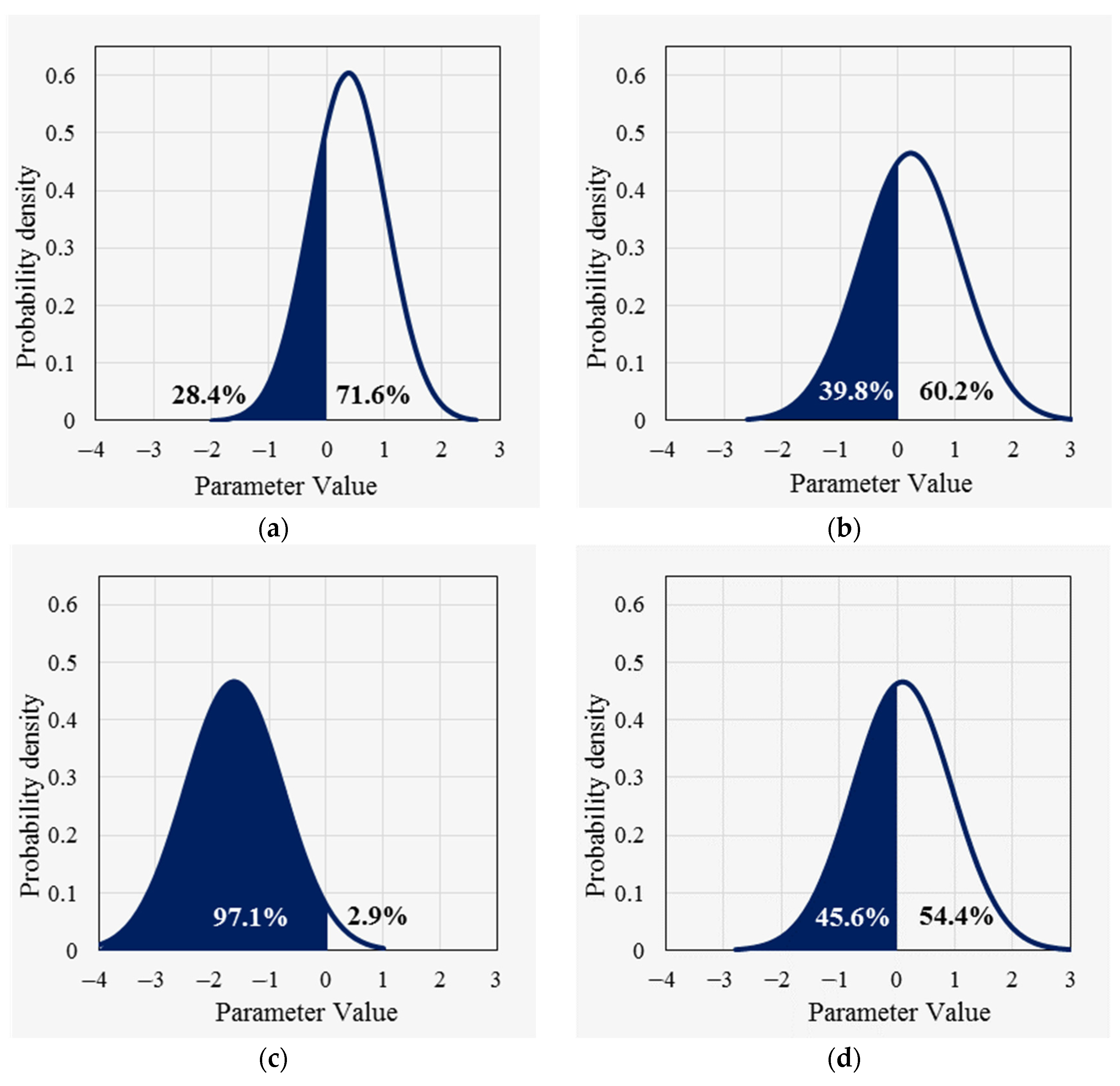
To further compare the differences between the two models, the parameter of the proportion of large trucks (PTV) is first used as an example to illustrate the effect of each factor on the mean value of the random parameters. In the basic random parameters model, this parameter follows a normal distribution with a mean of 0.376 and a standard deviation of 0.659 on all road segments, i.e., there is a 28.4% probability that the parameter will take a positive value and a 71.6% probability that the parameter will take a negative value on all road segments, as shown in Figure 1a. In the improved random parameters model, from Equation (36), the parameter follows a normal distribution with the mean () (i.e., the mean of the distribution of the parameter on each segment is not the same, depending on the values of the three variables of DSL, NL_4, and SAG) and the standard deviation of 0.857. For example, (1) for a steep uphill segment with four lanes and dual speed limits (NL_4 = 1, SAG = 1, DSL = 1), the parameter follows a normal distribution with a mean of 0.222 and a standard deviation of 0.857, as shown in Figure 1b; (2) for a steep uphill segment with four lanes and a single speed limit (NL_4 = 1, SAG = 1, DSL = 0), the parameter follows a normal distribution with a mean of −1.622 and a standard deviation of 0.857, as shown in Figure 1c; (3) for a nonsteep uphill segment with four lanes with various speed limits (NL_4 = 1, SAG = 0, DSL = 1), this parameter follows a normal distribution with a mean of 0.094 and a standard deviation of 0.857, as shown in Figure 1d.

Figure 1.
Distribution for the random parameter ; (a) Basic random parameters (RPs) model; (b) Case (1) for improved RPs model; (c) Case (2) for improved RPs model; (d) Case (3) for improved RPs model.
Further, the relationship between parameters and corresponding to the steep descending grade and the average distress ratio is analyzed. In the basic random parameters model, these two parameters follow normal distributions with mean values of 0.656 and −0.275 and standard deviations of 0.624 and 0.358, respectively, and the two distributions are completely independent of each other, as shown in Figure 2a,b. Whereas the results of the improved random parameters model show that the mean values of the two-parameters distributions are 0.684 and (−0.278 + 1.448 × DSL) and standard deviations of 0.614 and 0.402 (arithmetic square root of the diagonal elements in Table 3b), there is a significant correlation between the two distributions, with a covariance of 0.089 and a correlation coefficient of 0.361. The form of their joint distributions is shown in Figure 2c (the figure shows the roadway section where the DSL is = 0, i.e., a single speed limit).
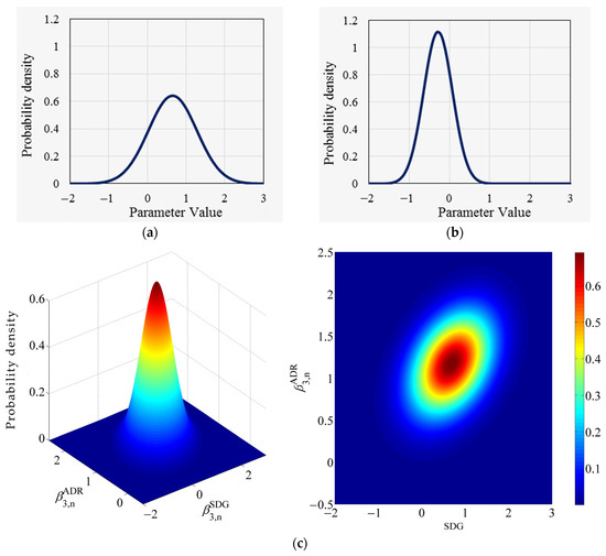
Figure 2.
Distribution for the random parameters and ; (a) Distribution of in basic RPs model; (b) Distribution of in basic RPs model; (c) Joint distribution of and in improved RPs model.
5. Evaluation of Statistical and Predictive Performance
5.1. Statistical Performance
The fixed parameters model, the basic random parameters model, and the improved random parameters model have the same modeling principle (in the form of the product of the total frequency of crashes and the proportion of crashes by severity) and model structure (based on negative binomial and multinomial logit models). Therefore, the statistical fit of these models can be compared by using the AIC, BIC, MacFadden ρ2 coefficient, and the Chi-square statistic χ2 [5,32].
The AIC, BIC, ρ2 coefficient, and other indicators of the above three models are summarized in Table 5, which show that (1) the statistical fit of the basic random parameters model is significantly better than that of the fixed parameter model (with lower values of LL(β), AIC, and BIC), which suggests that applying the random parameters can depict unobserved heterogeneity, and thus improve the model fit; and (2) on the basis of the basic random parameters model, further consideration of the variation in the means of random parameters, and at the same time, incorporation of correlations between random parameters, so as to account for unobserved heterogeneity, can further enhance the statistical performance of the model.
Table 5.
Statistical evaluation of the estimated models.
To further compare the goodness of fit of each model from a statistical point of view, the χ2 statistic between any two models was calculated, which is shown in Table 6. The results show that the basic random parameters model is significantly better than the fixed parameters model, and the improved random parameters model is significantly better than the basic random parameters model at a confidence level of 95%, which further verifies the reasonableness of the improved random parameters model estimated by this research.
Table 6.
The Chi-square statistics χ2 between estimated models.
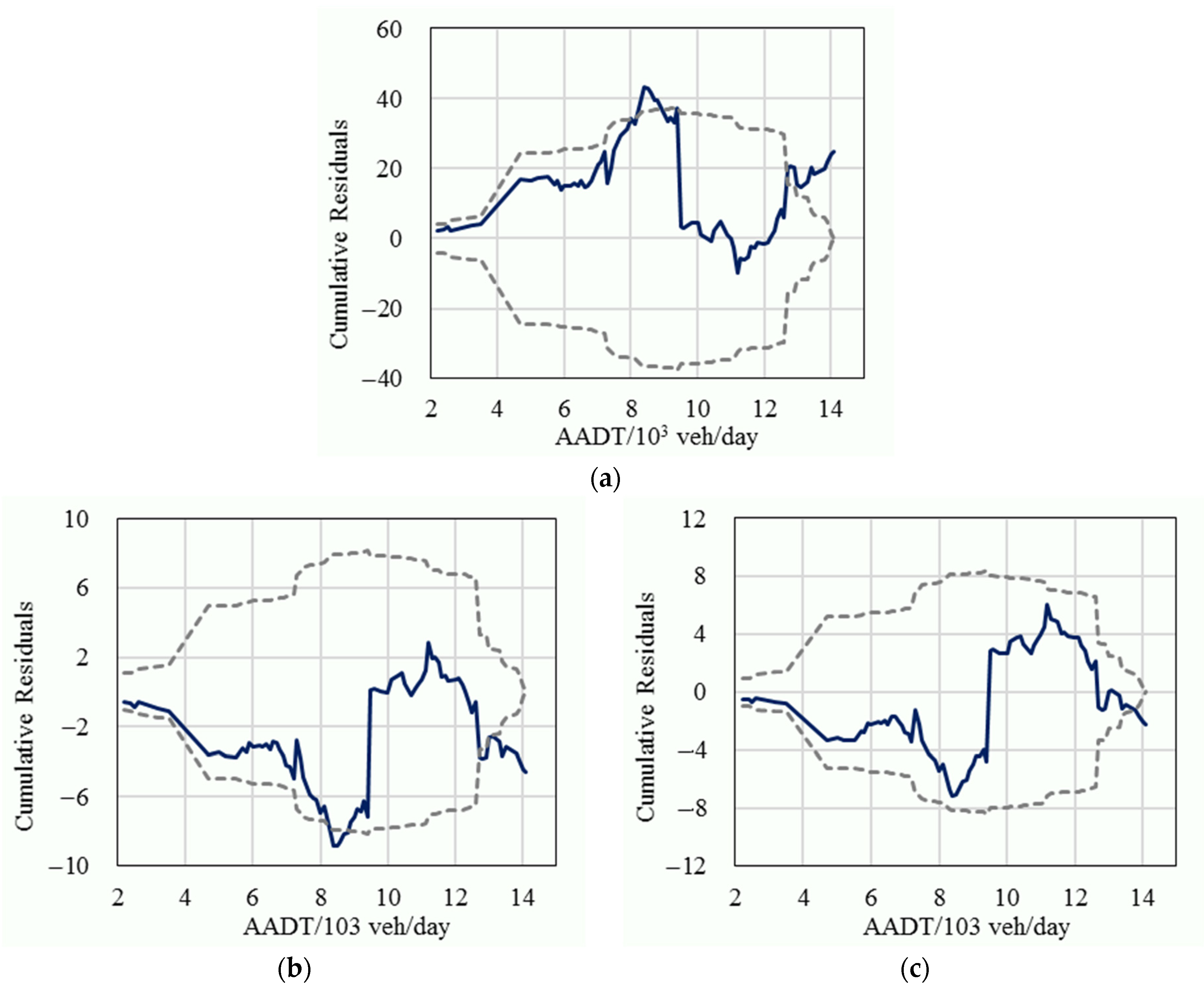
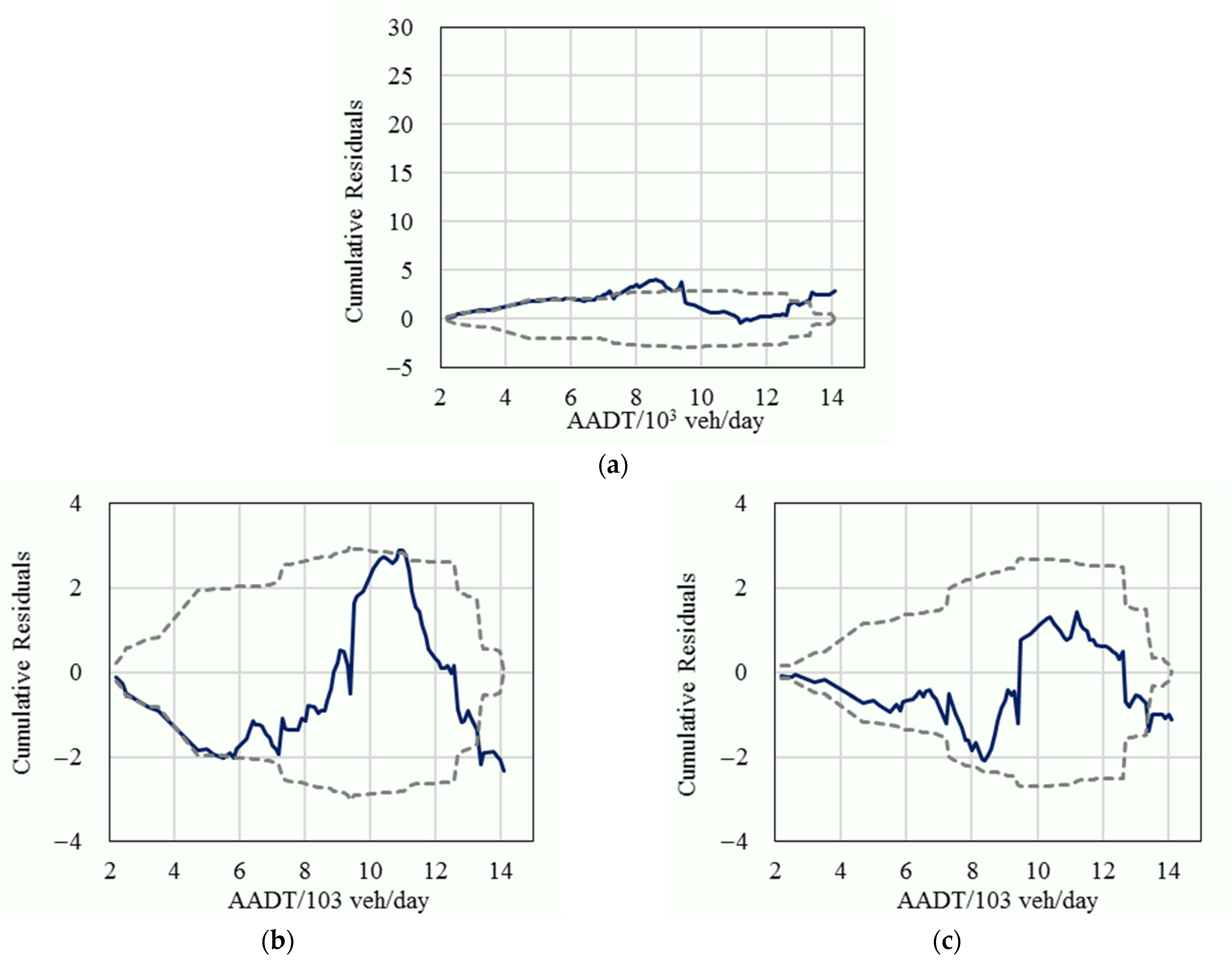
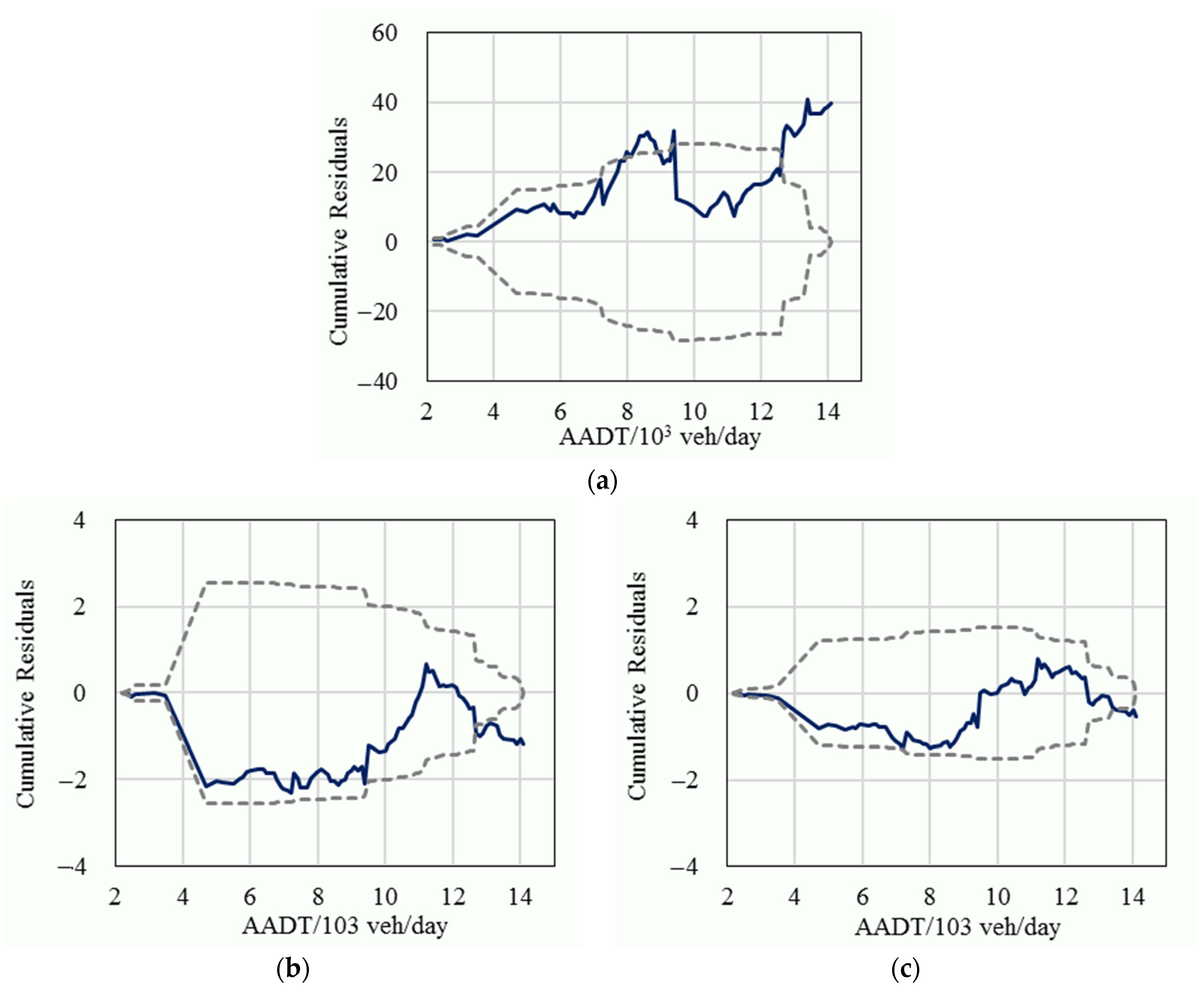
In order to further compare the statistical performance, the cumulative residuals of the fixed parameters model, the basic random parameters model, and the improved random parameters model for the variable of traffic volume were also calculated, as shown in Figure 3, Figure 4 and Figure 5. The results show that most of the cumulative residuals in the basic random parameters model did not exceed their 95% confidence intervals and were significantly better than the fixed parameters model. Compared with the basic random parameters model, all of the cumulative residuals of the improved random parameters model fell in their 95% confidence intervals (except for the tails), and their 95% intervals had a narrower range (which represents a more reliable result), which suggests that the improved random parameters model is superior to the conventional fixed parameters model and the basic random parameters model.
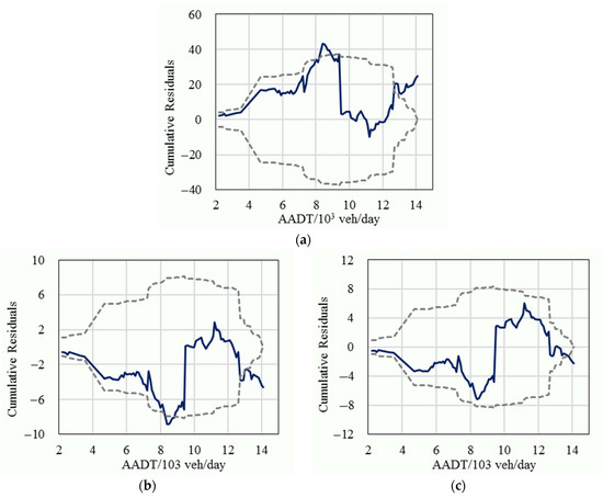
Figure 3.
The cumulative residuals (solid line) and their 95% confidence intervals (dashed line) for minor crashes; (a) The fixed parameters model; (b) The basic random parameters model; (c) The improved random parameters model.
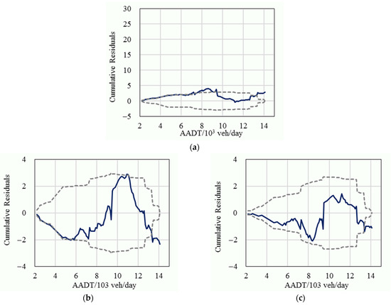
Figure 4.
The cumulative residuals (solid line) and their 95% confidence intervals (dashed line) for general crashes; (a) The fixed parameters model; (b) The basic random parameters model; (c) The improved random parameters model.

Figure 5.
The cumulative residuals (solid line) and their 95% confidence intervals (dashed line) for severe crashes; (a) The fixed parameters model; (b) The basic RPs model; (c) The improved RPs model.
5.2. Predictive Performance
In order to compare the estimated models from the perspective of prediction accuracy, the mean prediction error (MPE), mean absolute error (MAE), and root mean square error (RMSE) were calculated [32,33], as shown in Table 7. The results show that the MPE, MAE, and RMSE of the basic random parameters model are lower than the fixed parameters model for minor crashes, general crashes, or serious crashes. Compared with the basic random parameters model, the improved random parameters model can further improve the prediction accuracy significantly. For example, for minor, general, and serious crashes, the MPE can be reduced by 40–100%, the MAE can be reduced by 3.7–8.3%, and the RMSE can be reduced by 7.6–8.9%.
Table 7.
Predictive performance of various models.
6. Analysis of Safety Factors Based on Marginal Effects
6.1. Calculation Results of Marginal Effects
The marginal effects of the significant variables on the frequency of crashes by severity for the improved random parameters model were calculated, as shown in Table 8. In addition, to comparatively analyze the bias of the fixed parameters model and the basic random parameters model in terms of marginal effects, the results of these two models are presented together in Table 8. The results show that the marginal effects of the three kinds of crashes in the fixed parameters model have different degrees of bias, and the bias may exceed 100% for many factors (e.g., the proportion of large trucks, dual speed limits, and the steep ascending grade for general crashes, as well as the majority of variables for serious crashes), and the maximum bias can be up to −409% (the steep ascending grade for serious crashes). This shows that ignoring the unobserved heterogeneity may lead to serious bias. Compared with the fixed parameters model, adopting the random parameters approach to account for unobserved heterogeneity can largely reduce the bias, and the bias for the vast majority of factors is less than 100% (only the marginal effects of dual speed limits and steep ascending grade on general crashes and serious crashes have a bias of more than 100%), but the failure to incorporate the mean heterogeneity and correlation of random parameters caused by the interaction of safety factors results in the method still having a large bias (the bias of many factors exceeds 50%).
Table 8.
Marginal effects of significant variables on crash frequency by severity.
6.2. Analysis of Safety Factors Based on Marginal Effects
6.2.1. Factors with Fixed Parameters
The impact of various factors on crashes, traffic volume, and segment length, which are the exposure variables in the model for the total frequency of crashes, is positively associated with the frequency of crashes, which is in line with the basic principle of crash occurrence mechanism [19,22].
The tunnel segments are not as good as the basic road segments due to the lateral space and traveling environment [6,23], resulting in an average of 0.527, 0.444, and 0.069 more minor, general, and serious crashes on these road segments. As a result, reducing the speed limit, increasing the number of warning signs, and enhancing the lighting conditions for tunnels may be considered to improve traffic safety.
Regarding the type of speed limit, when dual speed limits are adopted on freeway segments (i.e., different speed limit values for large vehicles and passenger cars) these speed limits can reduce the average frequency of general crashes and serious crashes by −0.465 and −0.039, which can be attributed to the fact that the relatively lower speeds of large vehicles reduce the frequency of vicious crashes [16,22]. However, the lower speed of large vehicles often leads to an increase in the speed difference between different vehicle types, which, in turn, induces more overtaking and lane-changing behaviors, and, to a certain extent, also increases the frequency of minor crashes. Table 8 shows that the use of dual speed limits increases the average frequency of minor crashes by 0.145. However, overall, the adoption of dual speed limits is conducive to improving traffic safety and transportation sustainability, and the total frequency of crashes can be reduced by 0.359 (0.145–0.465–0.039), while the frequency of general and serious crashes can be significantly reduced. That is, adopting different speed limits for large trucks and passenger cars is recommended by this study, particularly when the volume of large trucks is high.
Regarding the number of lanes, as the number of lanes increases (provided that the traffic volume and other factors are certain), the number of crashes, on the contrary, tends to increase, potentially since the higher the number of lanes (from two to four), the higher the number of lane-changing and overtaking behaviors. This, in turn, increases the probability of crashes to a certain extent [19]. In practice, careful safety evaluation should be conducted to decide if widening a current freeway is more beneficial than constructing a new one. For existing freeways with multiple lanes in each direction, no passing regulation for risk segments may be considered.
In addition, for the variable of grade direction, the frequency of crashes on downhill segments is higher than that on uphill segments, especially on downhill segments where vehicles tend to engage in behaviors such as speeding. The results show that, on average, there are 1.264, 0.834, and 0.189 more minor, general, and serious crashes on downhill segments than on other segments. Hence, safety countermeasures should be considered to reduce vehicle operating speeds by adding speed limits or slow-down markings.
In addition, the rougher the road surface (the larger the international roughness index), the less favorable it is for safety (see the corresponding marginal effects in Table 8), while the larger the side friction coefficient, the greater the friction and lateral support that can be provided to the vehicle, and the more favorable it is for safety (reducing the probability of side-slipping and run-out-of-road crashes). In conclusion, the level of pavement maintenance not only affects the comfort of vehicle traveling but also greatly affects the level of traffic safety and transportation sustainability.
6.2.2. Factors with Random Parameters
For the proportion of large trucks, in general, the higher the proportion of large trucks, the higher the frequency of minor, general, and serious crashes. When the proportion of large vehicles increases from zero to one, the three types of crashes mentioned above will increase by an average of 0.691, 0.248, and 0.152 crashes, respectively, on each segment (average length of 0.554 km) over five years (the meaning of marginal effects of the other factors is also the same and will not be repeated). As a result, particular attention should be paid to freeways with a high volume of large trucks. For example, additional traffic warning signs or speed restrictions may be considered for these freeway segments. However, the parameters are random, indicating that the proportion of large trucks on each road segment exhibits random variation characteristics on the impact of crashes, and the mean value of the distribution of this parameter is correlated with the dual speed limits, steep ascending grade, and one-way four-lane segments. These factors have interactive effects on the frequency of crashes [30]. For example, as shown in Table 1 and Equation (36), the one-way four-lane (NL_4 = 1) road segments can effectively reduce the influence of the proportion of large vehicles on the frequency of crashes (the mean value of the random parameter is negatively correlated with the one-way four lanes). This is potentially because, when the number of lanes is large (more than four in one direction), large vehicles tend to be confined to travel in the outer slow lanes, which reduces the interference with small vehicles and reduces the vehicle overtaking behaviors, thus improving safety. Therefore, for freeways with four or more lanes in one direction, restricting the large trucks to the outside one or two lanes is likely to be an effective way to reduce crash risk and severity.
Compared with basic road segments, the frequency of crashes for the interchange/service-area segment is higher due to the existence of increasing behaviors of vehicle acceleration/deceleration and merging [19], which leads to a higher frequency of crashes. Table 8 shows that the frequency of minor, general, and serious crashes on the interchange/service-area segment is on average 0.215, 0.267, and 0.071 more than that on the basic segment. Therefore, the positions of warning signs for interchanges and service areas should be properly determined so that drivers can have sufficient time to avoid any potential crash risk. In addition, the parameter for this variable is random, indicating that there are unobserved factors related to the interchange/service area during the modeling process (e.g., ramp alignment, speed limit, and configuration of the interchange/service area, etc.), which result in differences in the frequency of crashes on different interchange/service-area segments.
The frequency of crashes increases with the increase of curvature, which indicates that sharp curves are better avoided when designing new freeways. For every one-unit increase in the curvature, the frequency of minor, general, and serious crashes increase by 0.230, 0.293, and 0.116, respectively, and the mean value of this parameter is negatively correlated with the steep ascending grade. The presence of a steep ascending grade (the marginal effect of the factor is negative in all cases) reduces the adverse effect of curvature on safety, potentially because of the complex road segments in combination with a steep ascending grade and sharp curves, where vehicle maneuvering is more difficult and sight distance conditions tend to be poorer, are somewhat conducive to traffic safety as drivers are more alert on such segments.
In terms of road pavement condition, the results show that a certain degree of distress (the maximum distress ration in this study is 4.25 percent) reduces the frequency of crashes of all types, potentially because drivers are more alert when traveling on these segments, thus reducing the probability of crashes. In addition, the crash risk increases with the increase in rutting depth, because deep rutting makes handling vehicles more difficult, particularly when changing lanes. These results emphasize the importance of road maintenance activities in order to improve both traveling comfort and traffic safety.
7. Conclusions
Traffic crashes are highly complex and influenced by a wide range of factors that interact with each other in an intricate manner. It is unlikely to cover all of the factors that affect the likelihood and severity of a crash for analysts, which inevitably brings unobserved heterogeneity. Ignoring unobserved heterogeneity can result in biased and inefficient safety inferences. To thoroughly account for unobserved heterogeneity when jointly modeling crash frequency by severity, the random parameters approach is introduced, and a basic random parameters model and an improved random parameters model are estimated along with a traditional fixed parameters model. The estimated models are comprehensively assessed from the statistical and predictive perspectives. In addition, to quantitatively analyze the impact of explanatory variables on the crash frequency of various severity levels, the calculating method of marginal effects for estimated models is proposed. The results show that the basic random parameters model statistically outperforms the fixed parameters model, and the statistical fit can be further improved by introducing heterogeneous means and correlation of random parameters, which indicates that accounting for unobserved heterogeneity can significantly improve the goodness of fit. For the predictive performance, the basic random parameters model is more accurate than the fixed parameters model, and the improved random parameters model can further reduce the mean error, mean absolute error, and root mean square error by 40–100%, 3.7–8.3%, and 7.6–8.9%, respectively. Regarding the safety analysis of factors, the results show that ignoring unobserved heterogeneity or neglecting the heterogeneity in means and correlation of random parameters may result in biased safety inferences, and the maximum bias of marginal effects can easily exceed 100 percent. In addition, the safety effects of explanatory variables are thoroughly discussed, and the potential safety countermeasures are provided. The random parameters approach used in this study is expected to provide a new methodological alternative to the joint analysis of crash frequency by severity. Furthermore, the innovative method for calculating marginal effects proposed by this study is believed to be vitally important, which is the foundation for uncovering the mechanism of crash occurrence and the resulting severity and making effective safety policies.
Undoubtedly, this research still has some limitations. The chief shortcoming is that the safety effects of variables included in the model may not be stable over the years. That is, temporal instability most likely exists as the five-year aggregated data are used in this study. Thus, future research can investigate the safety factors over time by using the method proposed by this study to gain more time-specific safety countermeasures. In addition, regarding the normal distribution of random parameters, only the heterogeneity in the means of the random parameters is tested. However, the variances of the random parameters may also be heterogeneous across observations and should be better investigated to gain more insights.
Author Contributions
Conceptualization, Z.C. and W.X.; methodology, Z.C. and W.X.; software, Z.C.; validation, Z.C., W.X. and Y.Q.; formal analysis, W.X.; investigation, Z.C.; resources, W.X.; data curation, Y.Q.; writing—original draft preparation, Z.C.; writing—review and editing, W.X.; visualization, Z.C.; supervision, Y.Q.; project administration, Y.Q. All authors have read and agreed to the published version of the manuscript.
Funding
This research was supported by the Fundamental Research Funds for the Central Universities, grant number 2572017AB26.
Institutional Review Board Statement
Not applicable.
Informed Consent Statement
Not applicable.
Data Availability Statement
Not applicable.
Conflicts of Interest
The authors declare no conflict of interest.
References
- WHO Global Status Report on Road Safety. World Health Organization. 2018. Available online: https://www.who.int/violence_injury_prevention/road_safety_status/2018/en/ (accessed on 20 July 2023).
- National Bureau of Statistics. China Statistical Yearbook of 2021. Available online: http://www.stats.gov.cn/zs/tjwh/tjkw/tjzl/202302/t20230215_1907978.html (accessed on 20 July 2023).
- Mannering, F.; Bhat, C. Analytic methods in accident research: Methodological frontier and future directions. Anal. Methods Accid. Res. 2014, 1, 1–22. [Google Scholar] [CrossRef]
- Mannering, F.; Bhat, C.; Shankar, V.; Abdel-Aty, M. Big data, traditional data and the tradeoffs between prediction and causality in highway-safety analysis. Anal. Methods Accid. Res. 2020, 25, 100113. [Google Scholar] [CrossRef]
- Hou, Q.; Huo, X.; Tarko, A.P.; Leng, J. Comparative analysis of alternative random parameters count data models in highway safety. Anal. Methods Accid. Res. 2021, 30, 100158. [Google Scholar] [CrossRef]
- Hou, Q.; Tarko, A.P.; Meng, X. Analyzing crash frequency in freeway tunnels: A correlated random parameters approach. Accid. Anal. Prev. 2018, 111, 94–100. [Google Scholar] [CrossRef] [PubMed]
- Rella Riccardi, M.; Galante, F.; Scarano, A.; Montella, A. Econometric and machine learning methods to identify pedestrian crash patterns. Sustainability 2022, 14, 15471. [Google Scholar] [CrossRef]
- Sharafeldin, M.; Farid, A.; Ksaibati, K. A random parameters approach to investigate injury severity of two-vehicle crashes at intersections. Sustainability 2022, 14, 13821. [Google Scholar] [CrossRef]
- Hou, Q.; Huo, X.; Leng, J.; Mannering, F. A note on out-of-sample prediction, marginal effects computations, and temporal testing with random parameters crash-injury severity models. Anal. Methods Accid. Res. 2022, 33, 100191. [Google Scholar] [CrossRef]
- Mahmud, A.; Gayah, V.V. Estimation of crash type frequencies on individual collector roadway segments. Accid. Anal. Prev. 2021, 161, 106345. [Google Scholar] [CrossRef]
- Afghari, A.P.; Haque, M.M.; Washington, S. Applying a joint model of crash count and crash severity to identify road segments with high risk of fatal and serious injury crashes. Accid. Anal. Prev. 2020, 144, 105615. [Google Scholar] [CrossRef]
- Hosseinpour, M.; Yahaya, A.S.; Sadullah, A.F. Exploring the effects of roadway characteristics on the frequency and severity of head-on crashes: Case studies from Malaysian Federal Roads. Accid. Anal. Prev. 2014, 62, 209–222. [Google Scholar] [CrossRef]
- Cai, M.; Tang, F.; Fu, X. A Bayesian Bivariate Random Parameters and Spatial-Temporal Negative Binomial Lindley Model for Jointly Modeling Crash Frequency by Severity: Investigation for Chinese Freeway Tunnel Safety. IEEE Access 2022, 10, 38045–38064. [Google Scholar] [CrossRef]
- Mannering, F.; Shankar, V.; Bhat, C. Unobserved heterogeneity and the statistical analysis of highway accident data. Anal. Methods Accid. Res. 2016, 11, 1–16. [Google Scholar] [CrossRef]
- Alogaili, A.; Mannering, F. Unobserved heterogeneity and the effects of driver nationality on crash injury severities in Saudi Arabia. Accid. Anal. Prev. 2020, 144, 105618. [Google Scholar] [CrossRef] [PubMed]
- Islam, M.; Alnawmasi, N.; Mannering, F. Unobserved heterogeneity and temporal instability in the analysis of work-zone crash-injury severities. Anal. Methods Accid. Res. 2020, 28, 100130. [Google Scholar] [CrossRef]
- Islam, M.; Hosseini, P.; Jalayer, M. An analysis of single-vehicle truck crashes on rural curved segments accounting for unobserved heterogeneity. J. Saf. Res. 2022, 80, 148–159. [Google Scholar] [CrossRef]
- Tahir, H.B.; Haque, M.M.; Yasmin, S.; King, M. A simulation-based empirical bayes approach: Incorporating unobserved heterogeneity in the before-after evaluation of engineering treatments. Accid. Anal. Prev. 2022, 165, 106527. [Google Scholar] [CrossRef]
- Hou, Q.; Tarko, A.P.; Meng, X. Investigating factors of crash frequency using random effects and random parameters models: New insights from Chinese freeway study. Accid. Anal. Prev. 2018, 120, 1–12. [Google Scholar] [CrossRef]
- Adanu, E.K.; Powell, L.; Jones, S.; Smith, R. Learning about injury severity from no-injury crashes: A random parameters with heterogeneity in means and variances approach. Accid. Anal. Prev. 2023, 181, 106952. [Google Scholar] [CrossRef]
- Chen, J.; Xu, M.; Xu, W.; Li, D.; Peng, W.; Xu, H. A Flow Feedback Traffic Prediction Based on Visual Quantified Features. IEEE Trans. Intell. Transp. Syst. 2023, 24, 10067–10075. [Google Scholar] [CrossRef]
- Rahman, M.M.; Islam, M.K.; Al-Shayeb, A.; Arifuzzaman, M. Towards sustainable road safety in Saudi Arabia: Exploring traffic accident causes associated with driving behavior using a Bayesian belief network. Sustainability 2022, 14, 6315. [Google Scholar] [CrossRef]
- Pervez, A.; Huang, H.; Lee, J.; Han, C.; Li, Y.; Zhai, X. Factors affecting injury severity of crashes in freeway tunnel groups: A random parameter approach. J. Transp. Eng. Part A Syst. 2022, 148, 04022006. [Google Scholar] [CrossRef]
- Hofer-Schmitz, K.; Stojanović, B. Towards formal verification of IoT protocols: A Review. Comput. Netw. 2020, 174, 107233. [Google Scholar] [CrossRef]
- Ijaz, M.; Liu, L.; Almarhabi, Y.; Jamal, A.; Usman, S.M.; Zahid, M. Temporal instability of factors affecting injury severity in helmet-wearing and non-helmet-wearing motorcycle crashes: A random parameter approach with heterogeneity in means and variances. Int. J. Environ. Res. Public Health 2022, 19, 10526. [Google Scholar] [CrossRef]
- Ijaz, M.; Lan, L.; Usman, S.M.; Zahid, M.; Jamal, A. Investigation of factors influencing motorcyclist injury severity using random parameters logit model with heterogeneity in means and variances. Int. J. Crashworthiness 2022, 27, 1412–1422. [Google Scholar] [CrossRef]
- Zubaidi, H.; Obaid, I.; Alnedawi, A.; Das, S.; Haque, M. Temporal instability assessment of injury severities of motor vehicle drivers at give-way controlled unsignalized intersections: A random parameters approach with heterogeneity in means and variances. Accid. Anal. Prev. 2021, 156, 106151. [Google Scholar] [CrossRef]
- Chen, J.; Wang, Q.; Cheng, H.H.; Peng, W.; Xu, W. A review of vision-based traffic semantic understanding in ITSs. IEEE Trans. Intell. Transp. Syst. 2022, 23, 19954–19979. [Google Scholar] [CrossRef]
- Hou, Q.; Huo, X.; Leng, J. A correlated random parameters tobit model to analyze the safety effects and temporal instability of factors affecting crash rates. Accid. Anal. Prev. 2020, 134, 105326. [Google Scholar] [CrossRef]
- Chen, Z.; Xu, W.; Qu, Y. Investigating factors of crash rates for freeways: A correlated random parameters tobit model with heterogeneity in means. J. Transp. Eng. Part A Syst. 2022, 148, 04021116. [Google Scholar] [CrossRef]
- Krichen, M. A Survey on Formal Verification and Validation Techniques for Internet of Things. Appl. Sci. 2023, 13, 8122. [Google Scholar] [CrossRef]
- Washington, S.; Karlaftis, M.; Mannering, F.; Anastasopoulos, P. Statistical and Econometric Methods for Transportation Data Analysis, 3rd ed.; CRC Press, Taylor and Francis Group: New York, NY, USA, 2020. [Google Scholar]
- Lord, D.; Qin, X.; Geedipally, S.R. Highway Safety Analytics and Modeling; Elsevier: Amsterdam, The Netherlands, 2021. [Google Scholar]
- Bhat, C. Simulation estimation of mixed discrete choice models using randomized and scrambled Halton sequences. Transp. Res. Part B 2003, 37, 837–855. [Google Scholar] [CrossRef]
- Shirazi, M.; Geedipally, S.; Lord, D. A Monte-Carlo simulation analysis for evaluating the severity distribution functions (SDFs) calibration methodology and determining the minimum sample-size requirements. Accid. Anal. Prev. 2017, 98, 303–311. [Google Scholar] [CrossRef] [PubMed]

Disclaimer/Publisher’s Note: The statements, opinions and data contained in all publications are solely those of the individual author(s) and contributor(s) and not of MDPI and/or the editor(s). MDPI and/or the editor(s) disclaim responsibility for any injury to people or property resulting from any ideas, methods, instructions or products referred to in the content. |
© 2023 by the authors. Licensee MDPI, Basel, Switzerland. This article is an open access article distributed under the terms and conditions of the Creative Commons Attribution (CC BY) license (https://creativecommons.org/licenses/by/4.0/).