Article

Simulation Study on Gas Leakage Law and Early Warning in a Utility Tunnel

School of Economics and Management, Beijing Jiaotong University, Beijing 100044, China
*
Author to whom correspondence should be addressed.
Sustainability 2023, 15(21), 15375; https://doi.org/10.3390/su152115375
Submission received: 24 August 2023 / Revised: 13 October 2023 / Accepted: 25 October 2023 / Published: 27 October 2023

Abstract

:
The large-scale construction of utility tunnels improves people’s daily life, but also increases the probability of gas leakage events. Gas is a flammable and explosive substance, and once a leakage and explosion accident occurs it will seriously affect the safety of personal property and disturb the urban order. Although the application of utility tunnels is becoming more and more widespread, the research on its operation and maintenance management is not sufficient. How to effectively and safely implement the operation and maintenance management of utility tunnels has become an important issue of concern for scholars at home and abroad. This paper takes the Beijing Winter Olympic Games utility tunnels as the research object, uses ANSYS Fluent R18.0, establishes the simulation model through the relevant fluid mechanics theory, and theoretically demonstrates the physical relationships of the relevant parameters. Through the simulation analysis of various leakage scenarios, the gas diffusion law is obtained when a small hole leaks, so as to determine the most economical and safest gas sensor deployment mode. The research results can provide theoretical support for the construction of utility tunnels in the future, provide ideas for the preparation of relevant system documents for utility tunnels, and ensure the orderly and scientific construction of utility tunnel projects.

1. Introduction

Utility tunnels are the inevitable product of urban modernization construction, the lifeline of urban life and industrial production, and play an important role in urban material transportation. When people use traditional pipelines to transport gas, they often employ shallow burial in the soil or overhead pipelines. These methods have many disadvantages, such as exposure to the soil, wind, and sun; pipeline rusting; cracking and corrosion; and other phenomena. When the pipeline is buried directly in the soil, it will have electrochemical reactions with various electrolytes in the soil. The application of utility tunnels effectively solves these shortcomings. However, gas leaks and explosions occasionally occur during the use of utility tunnels, and each accident causes serious losses of people and property. In order to effectively avoid gas pipeline leakage, it is very important to carry out scientific management of pipelines in utility tunnels.
With the emergence of modern utility tunnels, their advantages over traditional pipelines were soon shown and recognized worldwide. Cano-Hurtado et al. proposed that utility tunnels have many advantages, unlike traditional pipelines using open excavation [1]. The utility tunnel can effectively use underground space, avoid multiple excavations causing social disruption, and facilitate later maintenance. When a pipe fails, the overhauler is able to repair it in a timely and effective manner [2]. At present, due to the conditions of China’s large population base and small land occupation per capita, there is an urgent need for the rational utilization of underground space so that all types of resources can be transported safely and efficiently [3]. The application of utility tunnels can be a good solution to these problems. Some scholars have mentioned that there are many potential risks in the process of designing and applying utility tunnels. There are synergies between the various compartments, which are difficult to manage [4,5,6,7,8]. Kim et al. studied the accident factors by work type for highway construction projects through the analysis of accidents occurring in Korea from 1997 to 2008 [9]. Some scholars have proposed data-driven, simulation-based analytics to quantify the life-cycle cost of heavy equipment, incorporating both effectiveness and risks [10,11,12]. Arabi et al. proposed that the probability of success of construction projects is increased with the efficient management of key risks [13]. Scholars around the world have taken different research approaches to the various types of risks that may arise within utility tunnels to conduct research. Among the factors that contribute to the many risks in utility tunnels, gas leaks and explosions are undoubtedly one of the most influential. Once an accident occurs in a utility tunnel, the damage to production and life is significant.
Due to the relative complexity of gas leakage and explosion processes, there are many factors that can cause leaks, fires, and explosions. Scholars in various countries have conducted studies from different perspectives. Pilao et al. studied the effect of changes in multiple environmental factors on the occurrence of explosions in gas pipelines [14]. Some scholars have studied the combined effects of the area of the explosion, the location of the surrounding facilities, and the orientation of the fire on the utility tunnel [15,16]. Gas leaks are the root cause of both fires and explosions. There are many causes of gas leaks in utility tunnels. However, from the point of view of the damage caused by accidents, it is essential to effectively minimize the negative impact of gas leaks.
Academic research on gas leakage in pipeline corridors has focused on the possibility of gas pipeline explosions and the reasonableness of gas cabin construction. Scholars such as Fan studied how to reasonably design a ventilation system to achieve effective exhaust at different fire locations [17]. Yang et al. discussed the gas cabin development status of utility tunnels in China [18]. Some scholars have analyzed the effect of the process and location of laying pipe and the fan-room layout on the ventilation effect in the utility tunnel [19,20,21,22,23,24]. Wang et al. used the discrete element method (DEM) to simulate the process of fracture extension of concrete samples and the related mechanism analysis [25]. However, there is relatively little literature on gas leakage patterns and early warning response. Therefore, it is of great practical significance to study the basic rules of gas leakage.
In recent years, the numerical simulation approach has proven to be an effective method for studying utility tunnel accidents, not only with rigorous theoretical support but also in terms of cost to avoid the high cost of physical simulation. Therefore, it is widely used in the study of utility tunnels. Some scholars have investigated the fire characteristics of electrical power compartments under different ventilation methods. Experimental and numerical simulations found that the maximum roof temperature and smoke distribution in the corridor are closely related to the fire tightness and ventilation methods when a fire incident occurs [26,27]. Tang et al. studied the corresponding characteristics of a corridor body under strong seismic effects using numerical simulation as an example of a utility tunnel. The authors analyzed the influence of soil properties around the corridor body based on the seismic response [28]. Yang et al. investigated the effects of parameters such as the back arch height, reinforcement rate, and site conditions on the seismic performance of the corridor in a utility tunnel through shake table tests and simulation analysis [29]. Some scholars have investigated the fire and gas dispersion characteristics in a gas cabin with different ventilation methods and fire locations using a computational fluid dynamics (CFD) approach [30,31,32]. A reasonable simulation model is fast and economical in studying disaster risks and can provide a relevant theoretical basis for practical applications. Therefore, this paper also adopts the method of simulation analysis to analyze the gas leakage events in utility tunnels, so as to obtain the corresponding research conclusions.
A key part of gas leakage research is the construction of leakage models. The choice of leakage model is directly related to the accuracy of the simulation in depicting real-world leakage events. Before the emergence of integrated corridors, gas pipelines were mostly deployed by direct burial versus overhead pipelines, making the pipeline difficult to repair after a gas accident. The calculation of leakage models has also changed with the stage of development of the gas pipeline. Kunii and Levenspiel studied common disasters in storage tanks and pointed out that different measures should be taken depending on the caliber and shape of the leak and gave an effective formula for the calculation of the leak volume [33]. Montiel et al. studied a variety of overhead pipeline leakage scenarios and developed corresponding theoretical models to propose the calculation of leakage volume in the case of large-bore leakage [34]. Woodward and Mudan (1991) studied leakage scenarios when the pipe leakage size is small and used this to propose a small-hole leakage model [35]. In this paper, based on the simulation modeling of previous scholars, a comprehensive utility tunnel scenario is introduced and the relevant models are set up with strict physical relations, and finally the relevant gas parameters are statistically analyzed, which can provide a theoretical basis for the prevention of gas leakage.
In this paper, ANSYS Fluent R18.0 is used to simulate and analyze the gas leakage process in a utility tunnel. Since gas transportation belongs to the category of fluid mechanics in academia and the multiple packages built into ANSYS Fluent are the mainstream tools for analyzing fluid motion, it can be used for all industries related to fluids, heat transfer, and chemical reactions. ANSYS Fluent is suitable for the simulation analysis of pipe corridors because of its rich physical models, advanced numerical methods, and powerful preprocessing and postprocessing capabilities. Simulation with this software consists of three main steps: preprocessing, solver, and postprocessing. In the preprocessing stage, the corridor is modeled, its internal structure is defined by means of images, and the mesh is partitioned for the constructed image. In the solver stage, the mesh is checked for irrelevance, the boundary conditions of the model are set, and the mechanical model is applied. In the postprocessing stage, CFD Post R18.0 is used to analyze the data obtained from the simulation. With advances in computer performance and simulation techniques such as sub-fluent, the use of 3D numerical simulation of flow fields is becoming increasingly popular in industrial production and academic research.

2. Construction of a Comprehensive Pipeline Corridor Gas Simulation Model

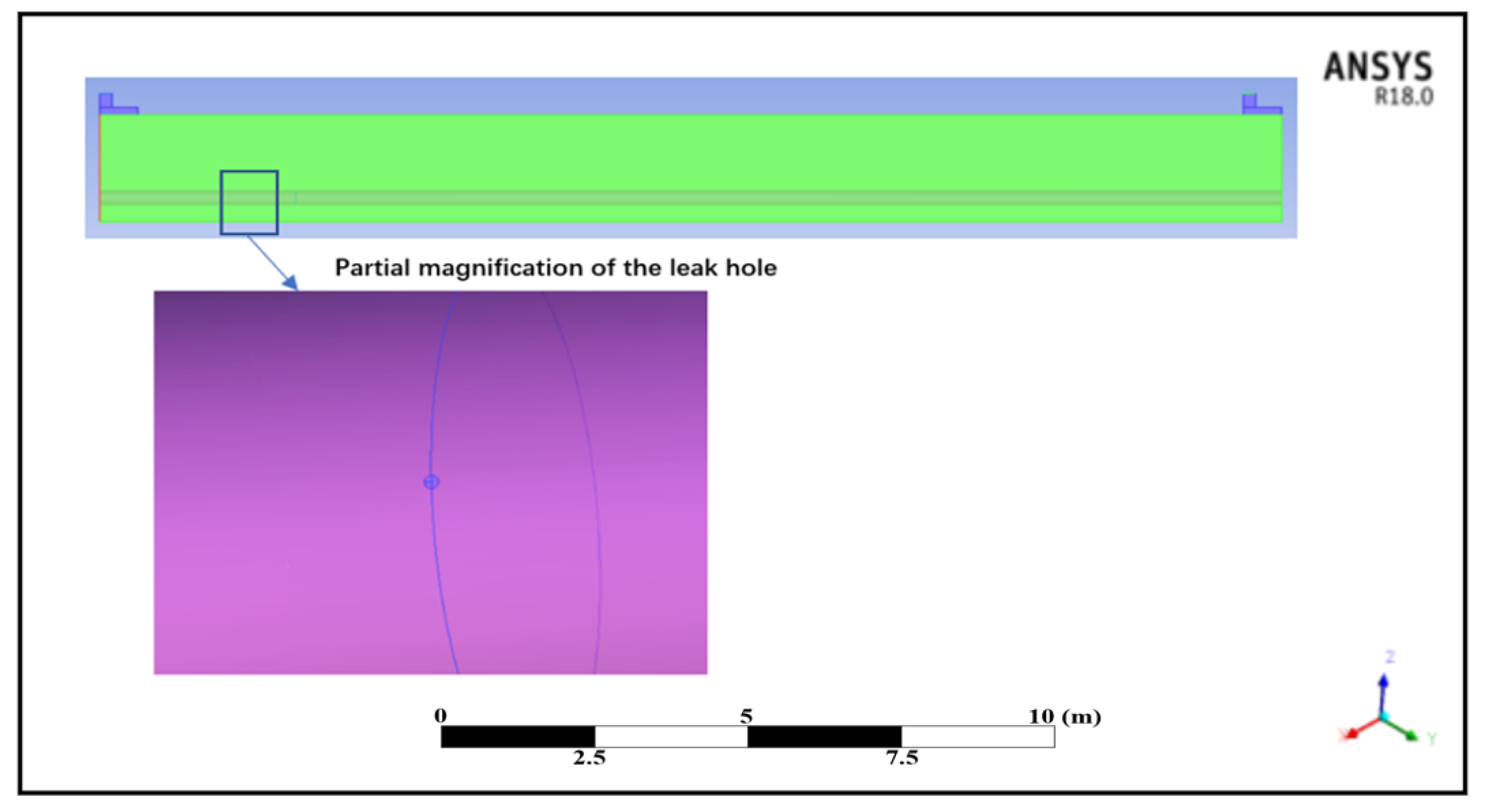
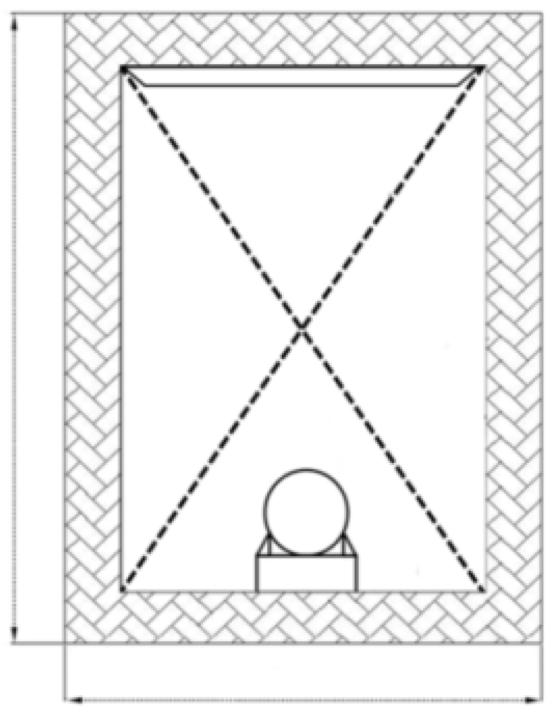
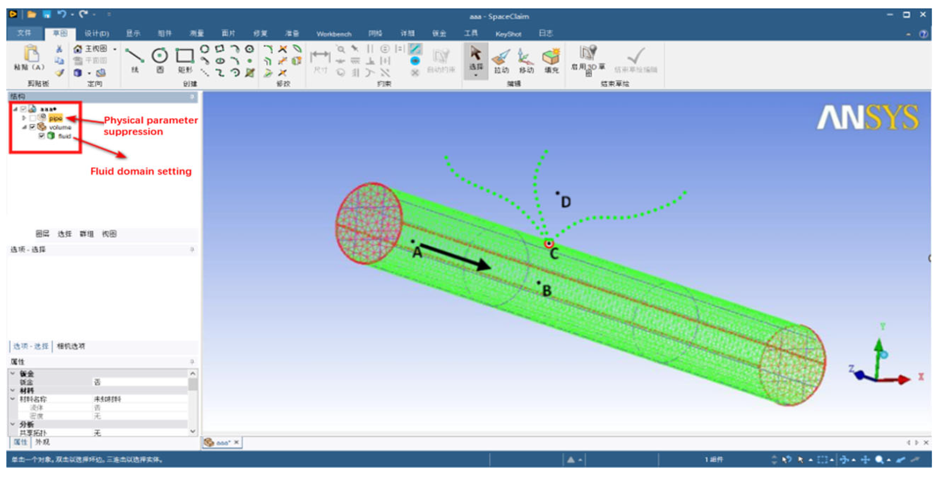
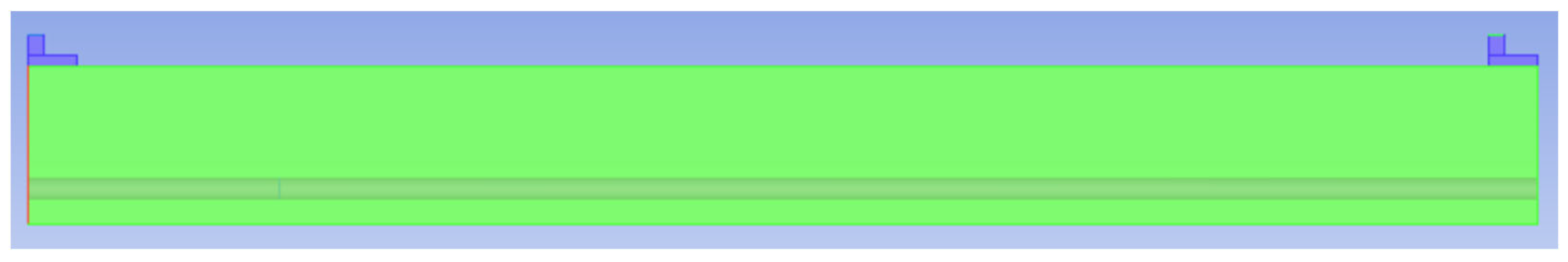
2.1. Physical Model Construction

This paper takes the utility tunnel engineering project used in the Beijing Winter Olympics venues as a physical research object. The utility tunnel in this area includes gas, water supply and drainage, and electricity cabins, as shown in Figure 1. This paper focuses on the simulation modeling analysis of the left gas cabin section. Since fire doors are set at fixed distances inside the corridor and the structure of the corridor body inside each section between the fire doors is roughly the same, this paper only studies the area inside two adjacent fire doors.
By measuring the relevant dimension data, ANSYS Fluent R18.0 is used to perform the model construction and parameter setting. The gas cabin model comprehensively considers the existing pipe fittings, including the gas pipe, pipe support frame, cabin wall, blower, air inlet, air outlet, air inlet interlayer, and air outlet interlayer. The specific size is as follows: the corridor length is 200,000 mm, the width is 1500 mm, and the height is 3000 mm; the diameter of the gas pipeline is 400 mm; the air supply outlet and exhaust outlet are 320 mm × 320 mm; and the leakage outlet is 2500 mm away from the air supply outlet in the vertical upward direction. The air supply outlet and exhaust outlet are equipped with interlayers, which are mainly used to study whether the gas will gather in the interlayer and fire door. The total volume of the space is 900 m3. The location relationship between the gas transmission pipeline and the cabin is shown in Figure 2. The model is designed based on Gambit 2.4.6, which can effectively help researchers build 3D models and design grid structures. This study assumes that gas is an incompressible fluid, and the standard k-ξ model is selected for its flow process. Additionally, the flow process of natural gas in this model is assumed to be in the form of turbulence, and the viscous effect between molecules is ignored.
The cross-section of the cabin can be a direct reflection of the relative position of the pipe in relation to other facilities within the cabin. The structural sketch of the cabin section is shown in Figure 3:
The gas pipeline is an important component in the utility tunnel, used for the transportation of materials, and it is is usually in the middle of the cabin. A simple diagram of the gas pipeline leakage model is shown in Figure 4.
Figure 4 provides the different take-off points and their positional relationships through a three-dimensional view of the gas pipeline. Different letters represent different leak locations:
A is the center point of the initial section of the gas pipeline, namely, the center point of the section where the valve is located;
B is the center point of the pipeline section where the leakage outlet is located;
C is the leakage point;
D is a point outside the pipe;
P, V, ρ, and T are the absolute pressure, velocity, density, and temperature of the state point, respectively.
As the main component of natural gas is methane, we simulate gas with methane in the simulation process. The simulation assumes that there is only a physical reaction in the process of gas diffusion without combustion and explosion. The physical dimensions of the leak hole remain constant throughout the leak process. The cabin pressure at point D can be approximately equal to the atmospheric pressure.
In this paper, two stages should be considered when calculating the gas leakage rate. The first stage is as follows: when gas leakage occurs, the gas supply is maintained continuously and the emergency valve is closed. The second stage is as follows: the emergency valve is opened and the remaining gas continues to leak until it stops. Due to the different physical environments of the two stages, different theoretical models and calculation methods should be adopted.

2.2. Calculation of Steady Leakage Rate of Gas Pipeline in Utility Tunnel

In this paper, the simulation study is concerned with the case where the leakage holes are small, i.e., the diameter of the leakage holes is less than 20 mm. Due to the small pore size, if the influence of the friction between the gas and tube wall is ignored, the gas expansion process is an isentropic process, and the leakage rate in this process can be considered to be constant. To facilitate calculation, some reasonable assumptions are made for the leakage process.
(1)
As shown in Figure 4, point “A” is a point far away from the leakage port, but the gas leakage speed is usually fast and there is not enough time to exchange heat with the environment. Therefore, point “A” to point “B” can be considered an adiabatic flow process of ideal gas.
T B = T A
(2)
From point “A” to point “B”, there is only one main pipe and no other gas flow outlet. The air pressure of urban gas is mostly below 1.6 MPa and the temperature is normal temperature. Therefore, the flow, pressure, and flow rate of the sections at point “A” and point “B” are not affected by the leakage outlet at all and satisfy the ideal gas state equation:
P ρ = R T  
P B = P A
In the above formula, definitions are as follows:
P is the absolute pressure (Pa);
ρ is the gas density (kg/m3);
R is the gas constant of CH4 (519 J/(kg·K));
T is the temperature of the gas (288 K);
P A is the pressure at point “A” in Figure 1 (Pa);
P B is the pressure at point “B” in Figure 1 (Pa).
(3)
According to The Urban Gas Design standards in China, when the nominal diameter of the gas pipeline in the comprehensive pipe corridor is DN200–300 mm, its corresponding wall thickness is 4.8 mm. The leakage process can be regarded as an adiabatic process due to the thin pipe wall and the high flow rate of the gas jet.
P ρ σ = C
d P ρ + v d v = 0
In the above formula, σ is the isentropic index of gas and is a function of temperature. At room temperature, the σ value of ideal gas can be approximately identified as a constant value. Since gas is a gas composed of polyatomic molecules, 1.29 is used. C is a fixed value and V is the average flow rate of the gas pipeline section (m/s).
By combining the above equations and making a calculation between points “B” and “C”, the following equation can be obtained:
v C 2 2 v B 2 2 = P B ρ B × σ σ 1 v d v 1 P C P B σ 1 σ
As the gas pipeline in this paper is DN200 mm and the aperture of the leakage outlet is less than 20 mm, v C >> v B , so v B 2 can be ignored. Therefore, Equation (4) can be simplified as:
v C = 2 σ σ 1 × P B ρ B 1 P C P B σ 1 σ
Then, the mass flow rate of small-hole leakage is:
q C = μ × S × ρ C × 2 σ σ 1 × P B ρ B 1 P C P B σ 1 σ
In the above formula, definitions are as follows:
q C is the steady state leakage rate, also known as the mass flow rate (kg/s);
µ is the flow coefficient (0.9–0.98);
S is the area of the leakage outlet of the gas pipeline (m2);
ρ C is the gas density at point C (kg/m3);
PB is the absolute pressure at point B (Pa);
PC is the absolute pressure at point C (Pa).
The value of pressure, PC, at the leakage outlet can be obtained from reference [5]:
P C = P a             ( P a > P E ) P E             ( P a < P E )
β = P c P B = 2 σ + 1 σ σ 1
In the above formula, definitions are as follows:
Pa is the pressure of the environment in the utility tunnel, equal to atmospheric pressure (Pa);
PE is the critical pressure (Pa);
β is the critical pressure ratio.
The critical pressure ratio refers to the ratio of gas pressure to stagnation pressure when airflow velocity is equal to local sound velocity, which is the transition point of gas jet velocity from subsonic to sonic velocity. At this time, the flow rate from the leakage hole is the critical speed. When P a / P B β , the jet flow at the leakage outlet of the gas pipeline belongs to the critical flow, P C = P a . When P a / P B > β , the jet flow at the leakage outlet of the gas pipeline belongs to the subcritical flow, P C =   P a .
When the gas leakage port is at critical flow, the critical velocity is:
v c = 2 σ σ 1 R T B
In combination with the adiabatic process of an ideal gas, the following formula exists:
T C T B = P C P B σ 1 σ
The maximum leakage flow at critical flow is:
q C = μ × S × P B R T B × 2 σ σ + 1 2 σ + 1 2 σ 1
When the flow at the leakage outlet of the gas pipeline is subcritical, the flow velocity of the gas at the leakage outlet and the maximum mass flow of the gas at the leakage outlet are, respectively:
v C = 2 σ R T B σ 1 1 P a P B σ 1 σ
q C = μ × S × P B R T B × 2 σ σ 1 P a P B 2 σ P a P B σ + 1 σ

2.3. Calculation of the Steady-State Leakage Time of the Gas Pipeline in the Utility Tunnel
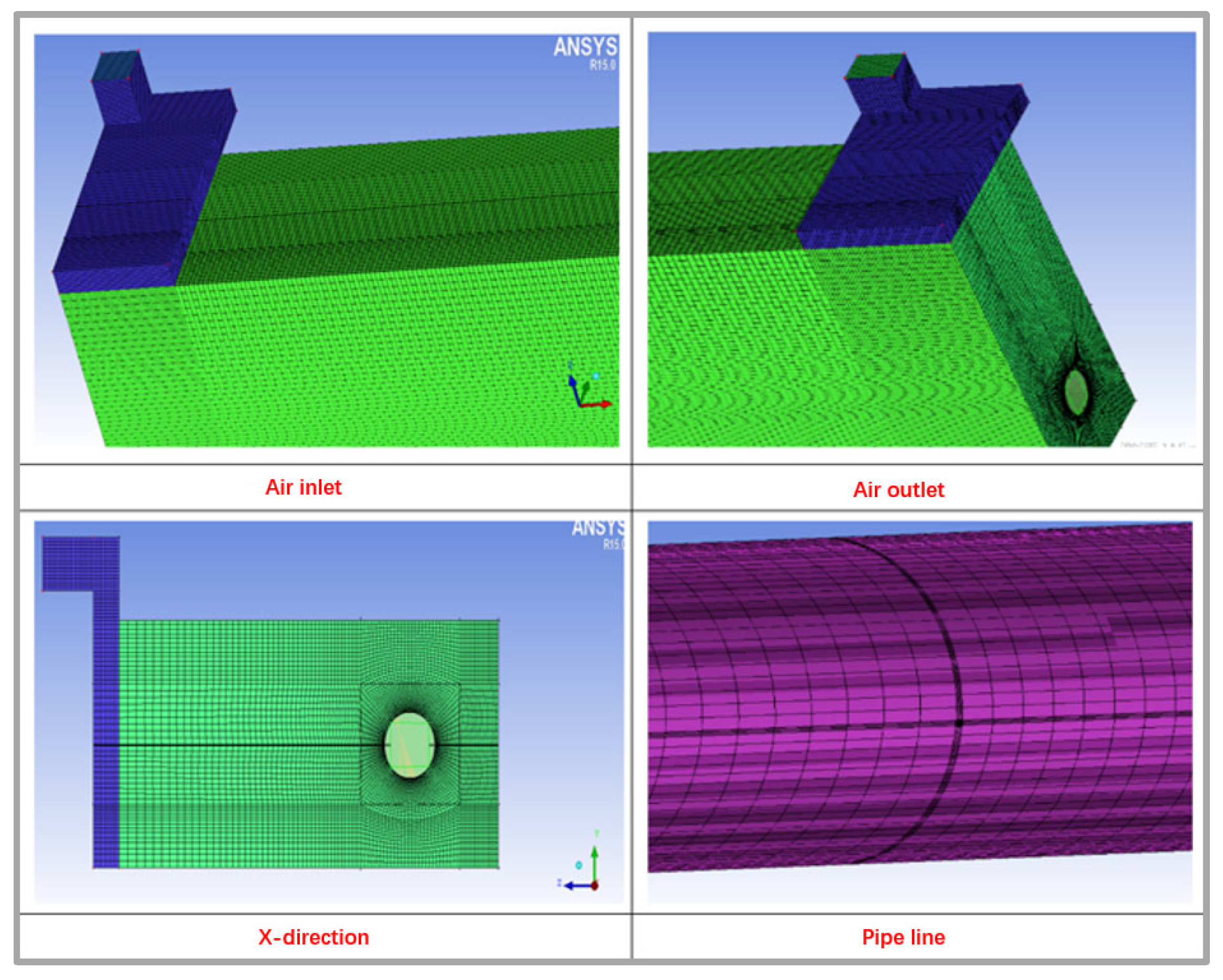
In order to reduce the damage caused by disasters, operators usually close the blocking valve in the gas pipeline immediately to cut off the supply of the gas source when gas leakage occurs in the utility tunnel. After the valve is closed, the gas pipeline located in the fire prevention zone can be regarded as a gas storage tank with a definite length and cross-sectional area, and the leakage model can also be regarded as a gas storage tank leakage model under a specific pressure. At this time, the density, gas flow rate, and pressure in the pipeline all change with time. The leakage process will change from critical flow to subcritical flow until the end of the whole leakage process.
According to the critical time, the time, t c , of the transition from the critical flow state to the subcritical flow state can be calculated as follows:
t a = 1 α 1 σ + 1 2 1 / 2 P a P 0 σ 1 / 2 σ 1
In above formula, definitions are as follows:
m 0 is the mass of residual gas in steady state (kg);
a is a function of m 0 and σ , a = Q m 0 σ 1 2 m 0 ;
P 0 is the pressure value of gas in steady state (Pa);
t is the moment of dynamic leakage (s).
Based on the above mathematical relations, the leakage time of critical flow can be obtained as follows:
t = P a P 2 1 γ 2 γ 2 γ + 1 1 2 1 2 m t q 0 γ 1
In above formula, definitions are as follows:
q 0 is the initial leakage rate of dynamic leakage (kg/s);
m t is the initial mass of gas in the area between adjacent shut-off valves (kg).
According to reference [5], when the dynamic leakage of polyatomic gas occurs, the subcritical leakage duration is approximately 2.333 times the critical leakage duration. Therefore, the following relationship can be obtained:
t Y = 2.333 t L
In the above formula, t Y represents the subcritical leakage time and t L represents the critical leakage time.

2.4. Grid Division

The model needs to be meshed before simulation calculations. In this study, ICEM CFD R18.0is used to create the grid division of the gas pipeline, support frame, air inlet, air outlet, related interlayer, and main corridor body in this section of the gas cabin. Due to the relatively small size of the interlayer and the inlet and outlet, gas will accumulate in this section. In addition, the size of the ventilation pipe is smaller than that of the main pipe cabin, so grid encryption is needed in these parts to ensure the accuracy of the results, as shown in Figure 5 and Figure 6. Considering the complexity of the overall pipe cabin structure, this paper adopts grid division technology combining structured grids and unstructured grids.
In the simulation process, the model mesh number density has a great influence on the results of the numerical calculations and the appropriate mesh number needs to be weighed by simulation accuracy, computation, and computer configuration. Therefore, this paper comprehensively considers many aspects and sets the grid nodes in the line grid stage. Then, factors such as skew angle, length–width ratio, node density, and node line smoothness were determined. In the mesh division method, the quad-map division method is selected and the corresponding mesh needs to have at least four faces. The vertices include at least four points of the type end, the remaining points are of the type side, and their corresponding mesh nodes must be equal in number. The fixed-point type and the node arrangement is set according to the division strategy. When refining the grid, it is adjusted according to the GAMBIT 2.4 software prompts, redrawing the grid fixed-point type and the number of nodes. If the grid still cannot be divided, the process switches to another division to redivide the grid for that region until all regions are divided. The division of the surface mesh and body mesh is similar to the above division method. When creating the pipe-wall mesh, maximizing the layer meshes of the boundary can effectively improve the calculation accuracy of the wall area and prevent the turbulent viscosity ratio from exceeding the defined value. In the block meshing stage, the smoothness of the mesh should be maintained at the adjacent parts of the chunks and the two meshes touching each other should be similar in size to avoid nonconvergence or the residual problem of the high continuity equation that occurs during the simulation calculation.
During the meshing process, some parameters need to be set in advance. Skewness is set to 0.5, change in cell size is set to 1.1, aspect ratio is set to 3:1, and the boundary layer is set to 6:1. The division of the gas cabin section mesh is shown in Figure 5.

2.5. Irrelevance Test of the Grid

The grid setting directly determines the accuracy of the simulation results, but an excessive number of grids can directly lead to a surge in computational effort. Therefore, it is necessary to check the mesh for irrelevance and find the right number of meshes. When the number of meshes continues to increase and reaches a certain value, the simulation calculation results no longer change. The number of meshes obtained at this point is the number of meshes that reach the irrelevance test.
Since this paper studies the gas diffusion law in utility tunnels, the focus is on the concentration values of gas leakage in each area of the corridor and the law of change. In the corridor, five measurement points are taken at appropriate distances and the gas concentration of each measurement point is calculated. Table 1 was obtained through testing.
As shown in Table 1, the gas concentration at points 1, 2, 3, 4, and 5 also continues to increase with the increasing number of grids. However, when the number of grids exceeds 5 million, the concentration value of each measurement point will not increase but will decrease, so 5 million is an appropriate number of grids. With the right degree of computational accuracy, it is possible to obtain the desired simulation results with less computational effort. Once the number of grids is determined, the relative relationship between the time step and grid compensation needs to be derived on this basis. The simulation results of gas leak concentration are closely related to these two factors. The Courant number is the intermediate quantity that links these two relationships to regulate the stability and convergence of the calculation. When the Courant number is larger, the convergence of gas concentration is faster, and vice versa. The larger the Courant number, the larger the simulation calculation of the gas concentration. Therefore, the size of the Courant number needs to be continuously adjusted until more accurate results can be obtained with the right amount of calculation. In the process of calculation, the Courant number is often set low and gradually increases according to the convergence of the iterative residuals. If the convergence rate is slow and stable, the size of the Courant number can be increased appropriately. Eventually, a more suitable Courant number is found, which can make the convergence fast enough and keep it stable.

2.6. Model Solving

In order to better analyze and compute the model in this paper, the selected solver is a pressure-based solver based on a coupled pressure–velocity coupled scheme, so a flow coefficient needs to be set to control the stability of the calculation during the solving process. In the iterative process, 10 is selected as the initial step of a grid, and then the simulation is solved for the gas concentration at each observation point. If there are observed points where the final concentrations do not converge, the grid step size is reduced appropriately and the concentrations are resolved for each point until convergence is reached at all points. The time step at this point is the final step, which is simulated to be 0.2 s.

3. Fluent Calculation Settings

3.1. Setting Up the Solver

During the computation of the simulation model, the computation of the flow field uses the spatially finite volume method, where the region is divided into many small volume cells by meshing, and the discrete control equations are solved on each volume cell. There are two main current solution methods. One is the pressure-based solution algorithm (press-based), which uses a pressure correction algorithm and can solve the control equations in scalar form with high accuracy for incompressible fluids. The other is the density-based coupled algorithm, which solves the control equations in vector form and is more accurate for solving the flow capacity of compressible fluids. Since the main component of the gas in the corridor is CH4, the pressure is 0.8 MPa, and the temperature of the pipeline carrying the gas is 288 K, it can be regarded as an ideal gas, treated as an incompressible fluid for simulation calculations.
In this paper, the coupled pressure–velocity equations are used in the solution process of the model through Fluent, and the specific algorithm is a separation solution algorithm. The pressure field obtained in each iteration does not fully satisfy the momentum equation, and iterations are needed until the results converge.

3.2. Setting of Boundary Conditions

Before using Fluent to perform simulation calculations, the boundaries of the model should be determined. Based on the object studied in this paper, the boundary conditions include the air inlet, air outlet, air inlet mezzanine, air outlet mezzanine, main corridor compartment, gas pipeline, and pipe support. In this paper, the temperature distribution is calculated by solving the energy control equation of the flow field, and the constant wall temperature is taken as the boundary condition. The overall model uses the k-ξ equation and the component transport equation. The environmental conditions set in the simulation are as follows: the gas pressure in the pipe is 1.6 MPa, the gas is an incompressible fluid, and the temperature in the pipe is 288 K.
As the outside of the cabin is connected to the outside space, the pressure of the gas cabin needs to be set to negative pressure in order to avoid gas leakage to other cabins through each exhaust duct and prevent combustion or explosion accidents in case of open fire or electric spark. The exhaust air is natural inlet and mechanical exhaust air, and the gas cabin air boundary conditions are velocity outlet and pressure inlet. The boundary conditions involved in the model are summarized in Table 2.
Turbulence intensity, a measure of the degree of velocity pulsation, is usually expressed as the ratio of the mean square of velocity fluctuations to the average velocity.
I = u V
In above formula, definitions are as follows:
u is the root mean square of the turbulent pulsation velocity, which is the standard deviation of the fluid velocity;
V is the average velocity (m/s).
u = 1 3 v x 2 + v y 2 + v z 2
Here, v x ,     v y , a n d v z are the components of velocity, V, in the x, y, and z directions, respectively (m/s).
Turbulence intensity:
I = 0.16 R e _ D H 0.125
Here, R e _ D H is the Reynolds number.
R e _ D H = u × D H v
Here, u is the flow rate, DH is the hydraulic diameter, and v is the kinematic viscosity.
D H = 2 R
Here, R is the hydraulic radius (m).
R = A X
Here, A is the cross-sectional area of the pipe, which is the ratio of flow rate to flow rate (m2). X is the wet perimeter, which is the perimeter required for the fluid to flow through the outer ring of the pipe for one wet week (m).

4. Study on the Diffusion Radius of Gas Leaks in Utility Tunnels

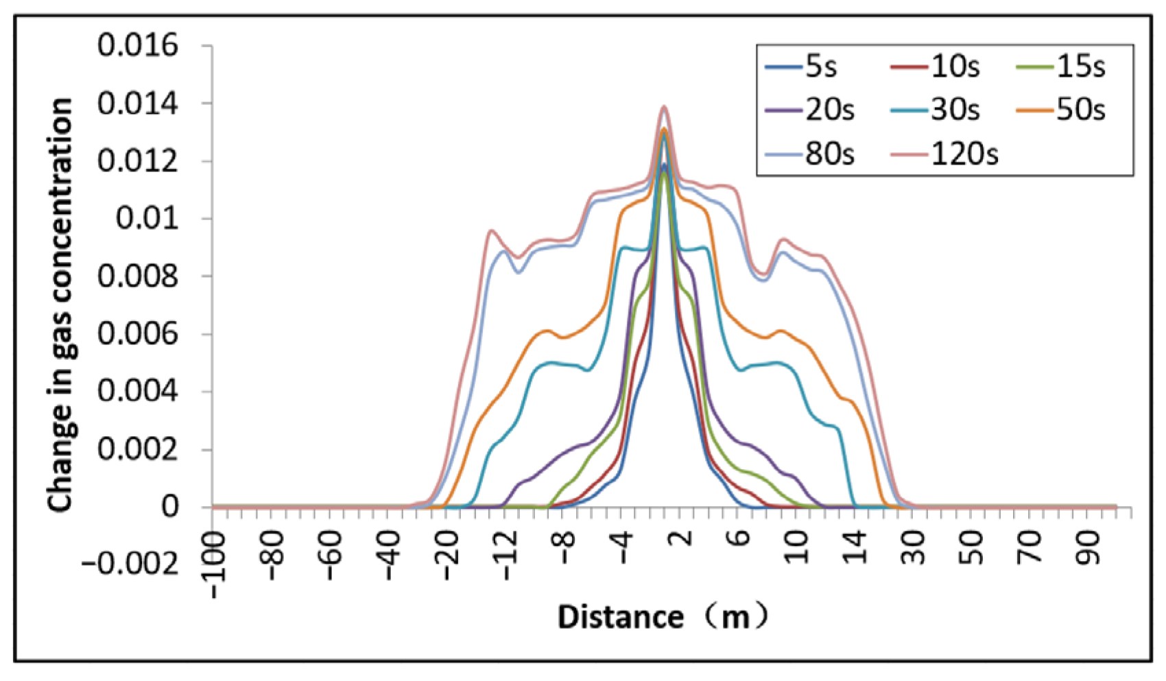
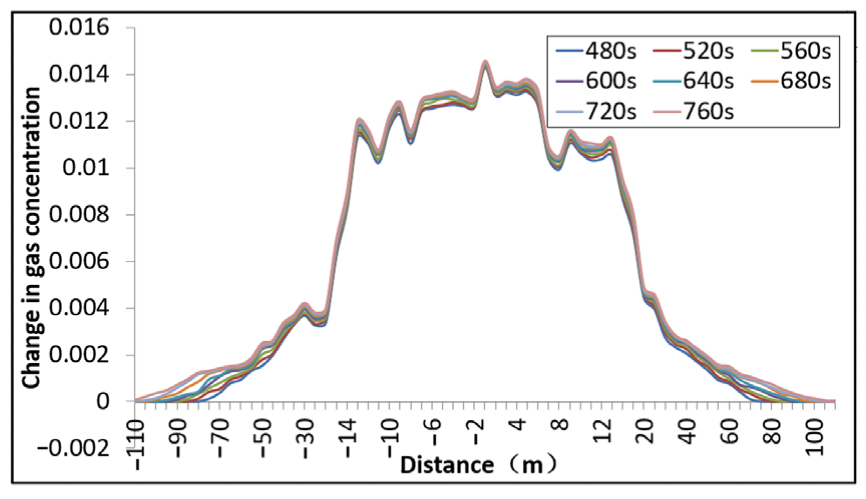
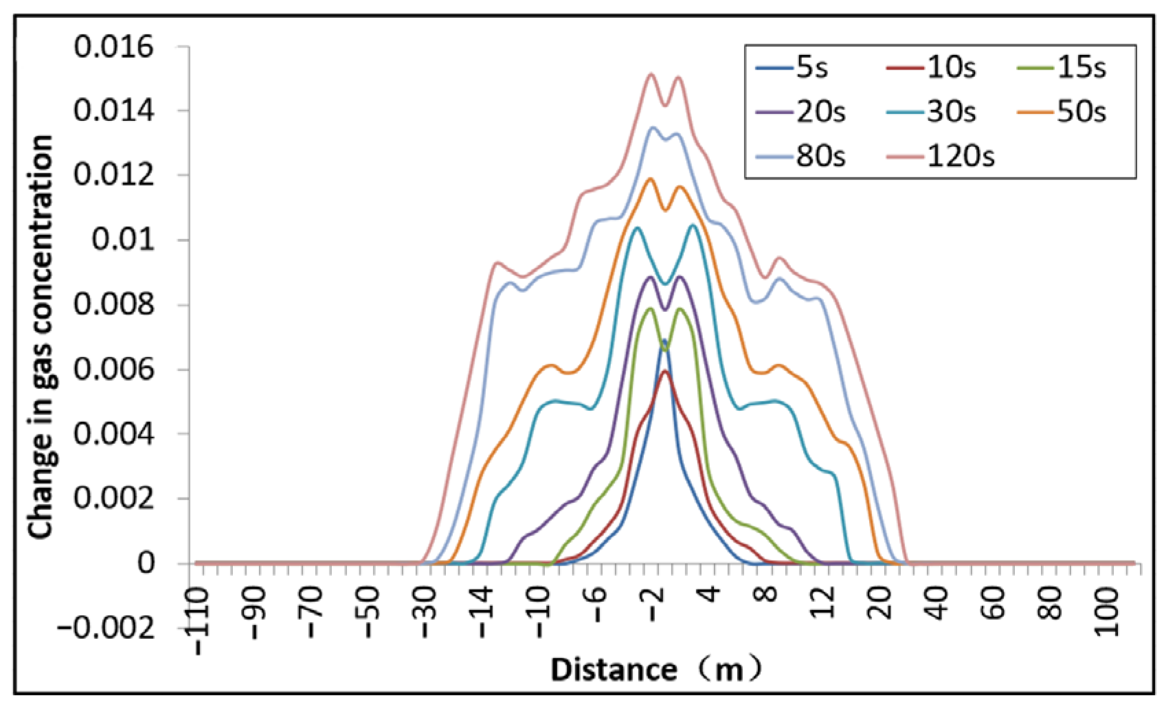
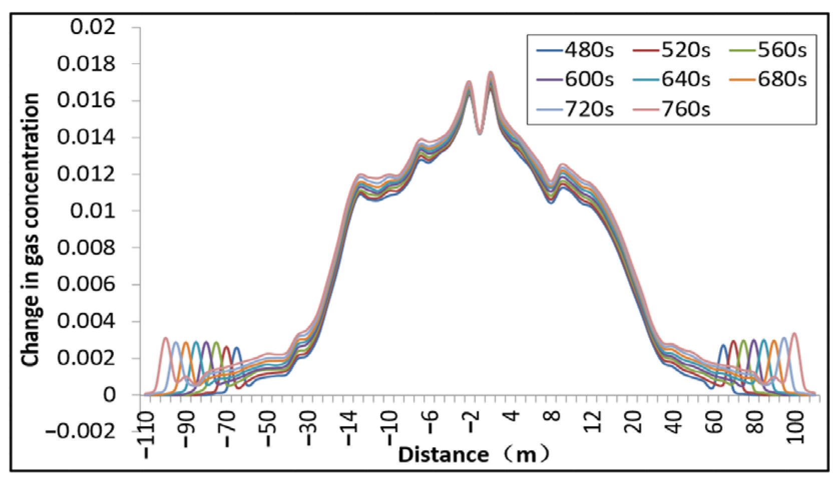
4.1. Graph of the Gas-Leak Radius over Time

As the concentration of gas in the gas cabin varies from point to point during the gas leak, the dispersion pattern presented at different heights is different. Therefore, for the convenience of comparison, two observation lines are taken in this paper, which are the centerline located at the center of the gas cabin space and the observation line 0.2 m from the top of the pipe gallery. The main component of the gas in the gas pipeline is CH4, which is prone to explosive accidents when encountering open flames or electric sparks. Gas itself is toxic, and how to effectively determine the gas in the leakage accident diffusion law is directly related to the accident handling measures and the ultimate size of the loss. This section conducts a simulation study of gas leakage events at normal transport concentrations, defining the hazardous area in the cabin by the concentrations at each observation point to determine the leakage pattern of gas during the leakage from small holes.
Based on the actual situation, the gas leakage event is simulated and analyzed, and the leakage hole size is set as a circular hole with a diameter of 5 mm. The current pipeline pressure is 1.2 MPa, there is no mechanical ventilation, and the minor influence of the pipeline support on gas diffusion is not considered. In the study of the gas dispersion radius, two observation lines are taken for comparison. The time axes of both observation lines take values ranging from 0 to 760 s, and the corresponding concentration changes are shown below.
As we can see from Figure 7, Figure 8 and Figure 9, under the 1.2 MPa condition with no mechanical ventilation, the leakage of 5-mm diameter leakage holes in both observation lines is not completely symmetrical. The leak radius is 7.1 m at 5 s, 8.3 m at 10 s, 10.2 m at 15 s, 12.1 m at 20 s, 14.4 m at 30 s, and 22.3 m at 50 s. The leak radius at 5 s is 7.1 m, 8.3 m at 10 s, 10.2 m at 15 s, 12.1 m at 20 s, 14.4 m at 30 s, and 22.3 m at 50 s. In the first 50 s, the leak radius is essentially symmetrical around the leak point. At 0–20 s, the maximum concentration of gas in the cabin is approximately 0.0125; the measurement was taken directly above the leak. At 20–120 s, the maximum concentration of gas in the cabin continues to rise, reaching approximately 0.0139 at 120 s, and the rise rate of the whole process is faster than before. At 120–440 s, the rise rate is smaller and finally reaches approximately 0.0142. At 480–760 s, the maximum gas concentration remains basically unchanged.
The distance of the leak from the two ends of the gas cabin is different, and this effect will gradually expand over time, which in turn will lead to some changes in the gas leakage pattern at each point. At 80 s, the gas concentration in the range of 0–10 m to the left of the leak changes slowly, the 10–12-m section trend is first decreasing and then increasing, and the 12–25-m section trend is rapidly decreasing from a higher concentration to 0. The decreasing trend is basically a linear relationship. At 0–8 m to the right of the leak point, the leak concentration gradually decreases from high to low, and in the 8–12-m section, the gas concentration first rises to a higher concentration and then decreases to the previous concentration with local symmetry. From 12–25 m to the right of the leakage point, it also decreases rapidly from a higher concentration to 0, and the decreasing trend is basically linear.
At the moment around 400 s, the gas concentration does not change much at 15–29 m on the left side of the leak hole and shows a slow decreasing trend, while the right side of the leak hole shows a similar pattern at 11–15 m. After additional time, the interval of the slow downward trend on the left side gradually shortens, while the right side remains unchanged.
It is easy to see from Figure 10, Figure 11 and Figure 12 that, over time, the concentration of each observation point in the cabin continues to increase, and the gas diffusion radius gradually increases from the leak point. However, the diffusion rate gradually decreases, and the gas concentration at the final leak point is basically maintained at approximately 0.014. At 760 s, the gas diffusion radius reaches 110 m, which exceeds the actual fire zone length of the cabin, and the simulation model stops when it reaches the termination condition.
The concentration of observation line 2 is theoretically larger than that of observation line 1 because it is closer to the leak. After conducting simulation tests, however, a more complex pattern was found. At 5 s, the maximum concentration of observation line 2 is 0.0064, while the maximum concentration of observation line 1 at this time is 0.0118, at which point the maximum concentration of observation line 1 is less than the maximum concentration of observation line 2. The leakage radius at 5 s is approximately 7.1 m, which is basically consistent with observation line 1. At 10 s, the highest concentration of observation line 2 is approximately 0.00061, which is slightly lower than that at 5 s and smaller than the corresponding concentration of observation line 2 at that time. After 10 s, the concentration at each point on observation line 2 continues to increase, and the image of the concentration leakage is basically symmetrical around the leakage point. A decreasing trend of concentration was observed from the highest concentration to both ends of the cabin until 240 s. However, after 240 s, the concentration in part of the area away from the leak increases and is higher than the concentration in the surrounding area. This is because, after the gas leaks from the hole, it will first gather at the top of the cabin and spread from the middle to the ends. When the top gas reaches the ends of the cabin, it will settle, making the concentration of gas at the far end higher.
As shown in Figure 13, the concentration diffusion radius trend of observation line 1 and observation line 2 is approximately the same, gradually increasing with time, and the diffusion rate is both fast and then slow. In the leakage time interval [0, 50 s], observation line 1 and observation line 2 are basically coincident. The concentration spread radius on observation line 2 is always greater than the concentration spread radius on observation line 1 during the leakage time interval [50, 600 s]. At the leakage time interval [500, 800 s], the concentration of observation line 2 is lower than that of observation line 1. This is because observation line 1 is at the top of the cabin and when the leaking gas gradually increases it will spread at the top toward the ends of the cabin, and when it reaches the ends of the cabin the gas sinks downward due to the squeezing effect. Therefore, at the far end, the concentration of observation line 1 is lower than that of observation line 2, while the concentration at the remaining points is basically higher than that of observation line 2. The growth rate of the gas diffusion radius is first fast and then slow, which is related to the pressure difference between the inside and outside of the pipe. As the gas diffuses, the concentration of gas in the cabin begins to increase and the pressure difference between it and the gas in the pipe decreases, which in turn leads to a decrease in the growth rate of the diffusion radius of the gas.

4.2. Influence of Leak-Hole Diameter on Diffusion Radius

The above analysis shows the leakage pattern for a 5-mm diameter leak hole, but the size of the bore directly affects the leakage rate and the gas pressure. In order to investigate the effect of leakage holes of different diameters on the gas leakage pattern, we studied leakage holes with diameters of 4 mm and 6 mm under the same simulation parameters described above.
According to Figure 14, when the size of the pipe leakage hole increases, the leakage radius at a certain point also increases, but the rate of increase gradually decreases. This is mainly due to the larger leak hole and the larger pressure difference between the inside and outside of the gas pipe at the starting moment, resulting in a larger gas flow per unit time, which in turn makes the gas-leak radius larger. However, as the leak volume increases, the pressure difference between the inside and outside of the gas pipe gradually decreases, eventually leading to a slow decrease in the leak rate. When the leak-hole size is reduced, the gas-leak radius is also reduced accordingly. As the leakage hole used in this paper represents small-hole leakage, when the diameter is reduced by 1 mm, the area is only 64 percent of the previous one, so it has a greater impact on the leakage radius, and the leakage rate still keeps the law of first fast and then slow.
Similar to observation line 1, the radius of leakage on observation line 2 also increases with increasing leakage aperture. The increase is related to the relative proportion of the area change; when the leak hole is reduced by 1 mm, the area is 0.64 times that of the previous one. However, when the leak hole is increased by 1 mm, the area is 1.44 times that of the previous one. Therefore, the change in the leakage radius is more pronounced for an increase of 1 mm.

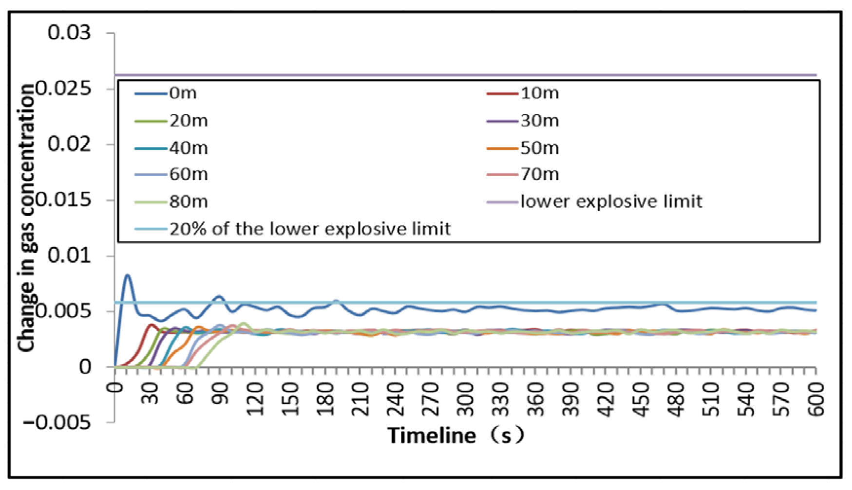
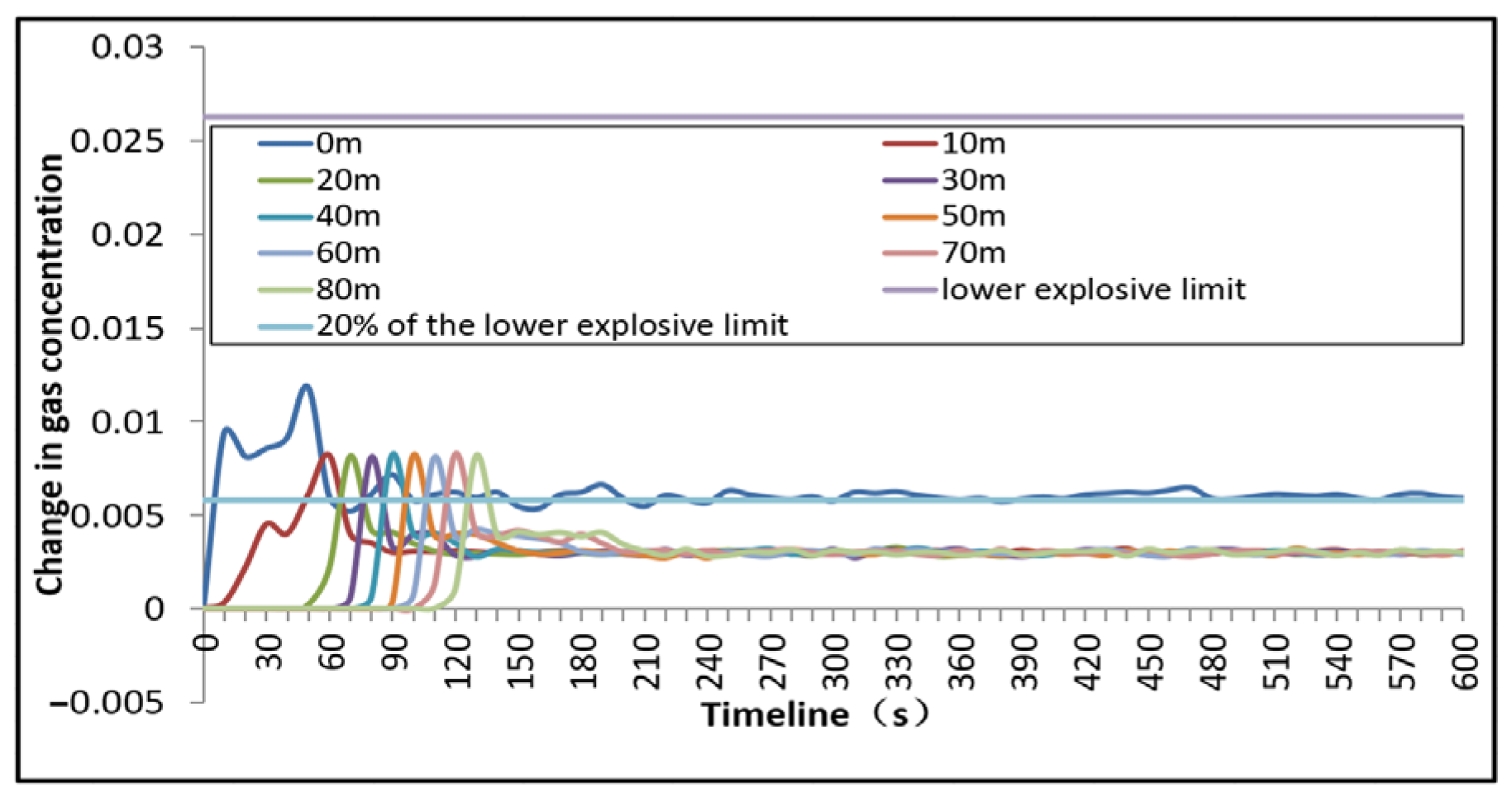
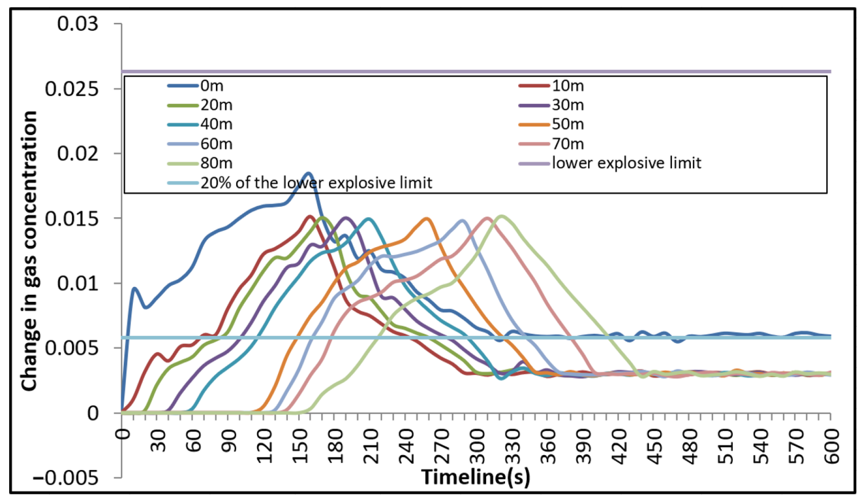
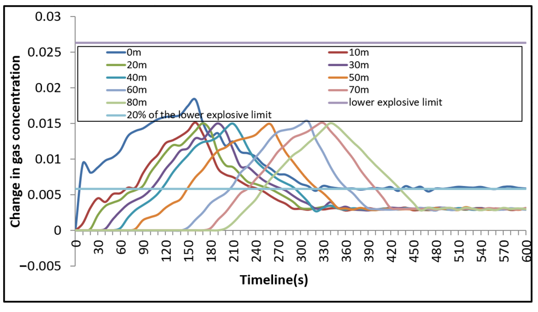
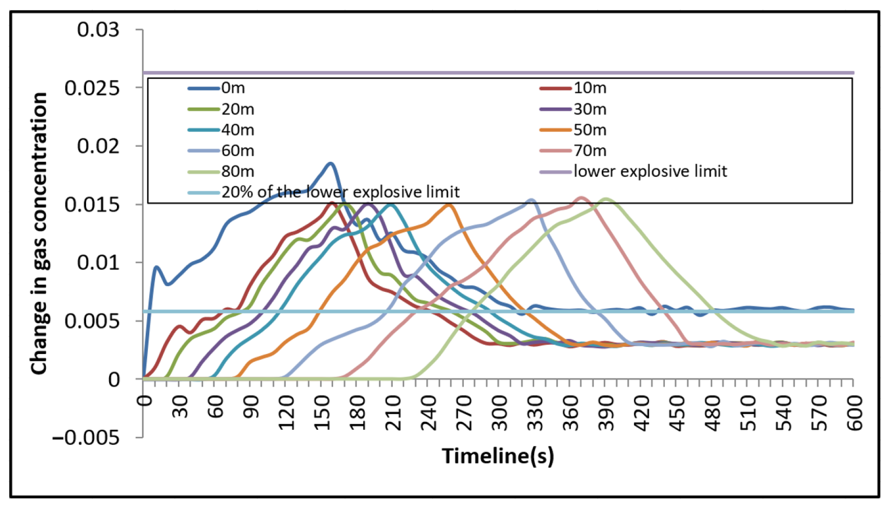
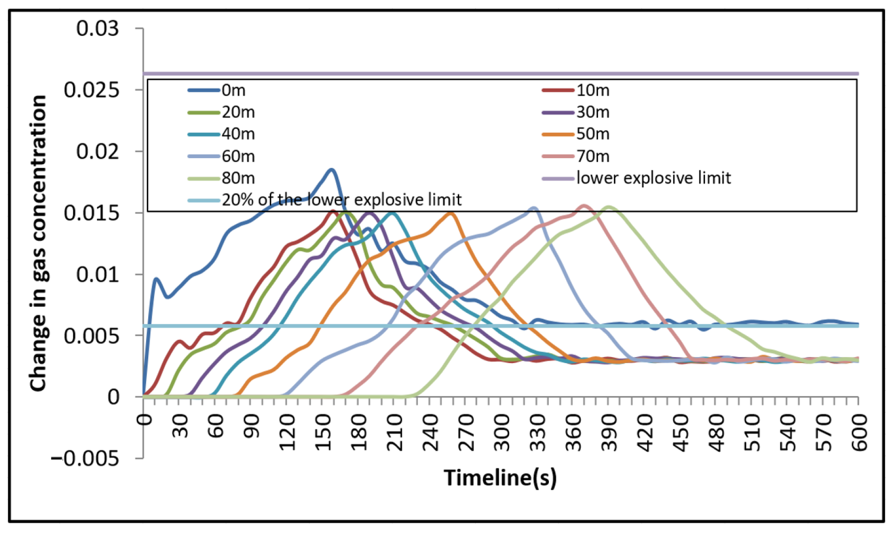
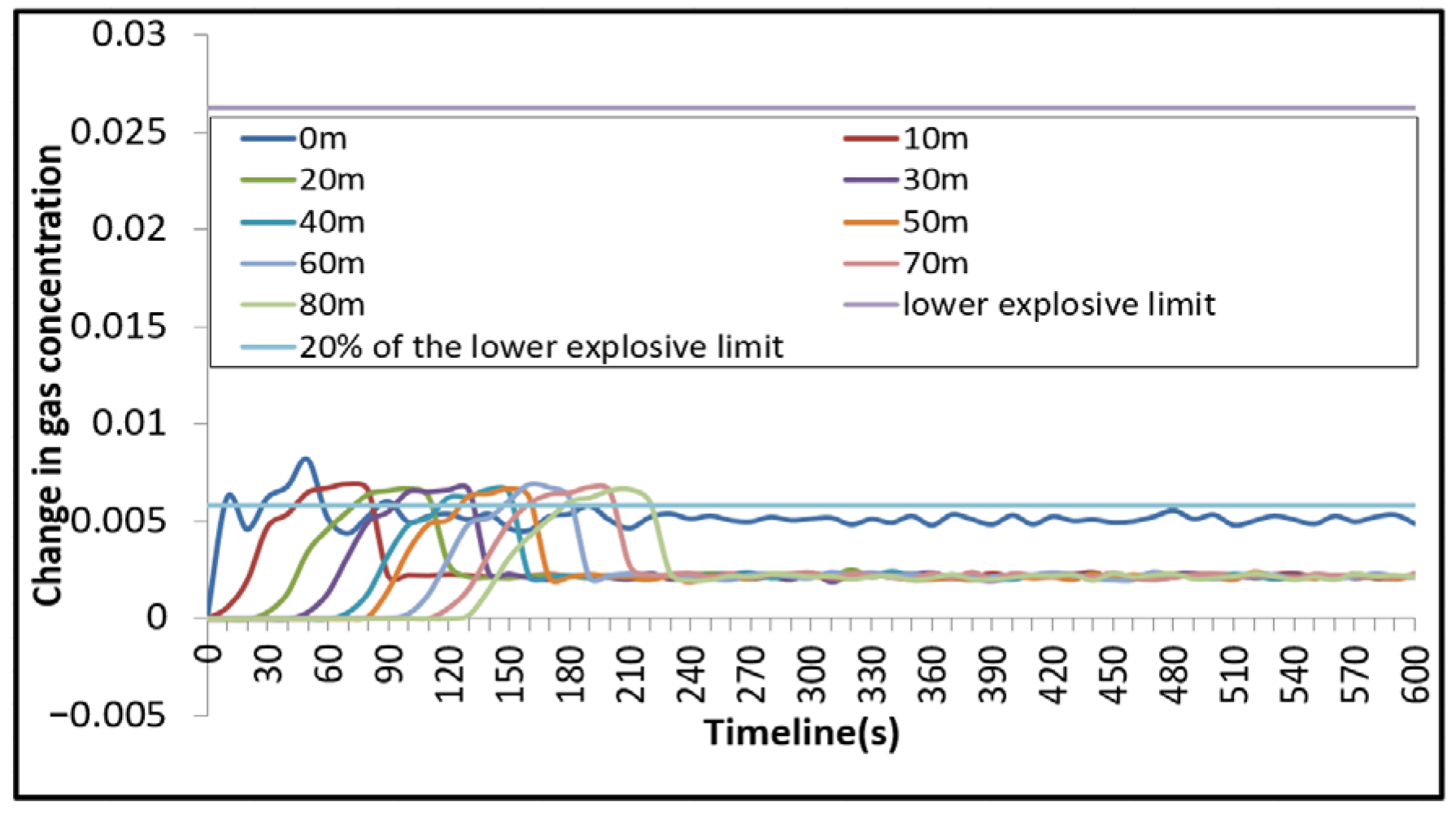
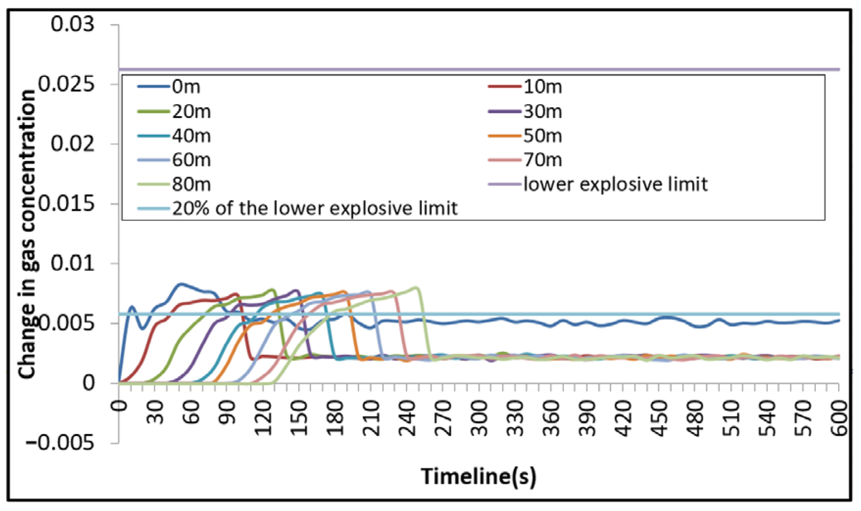
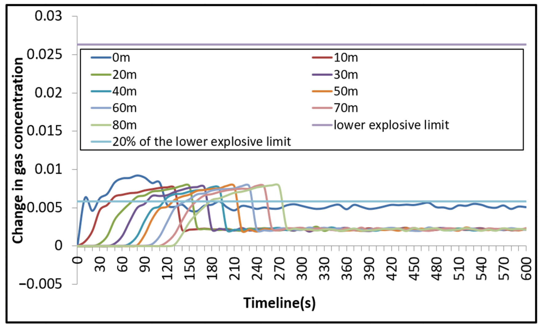
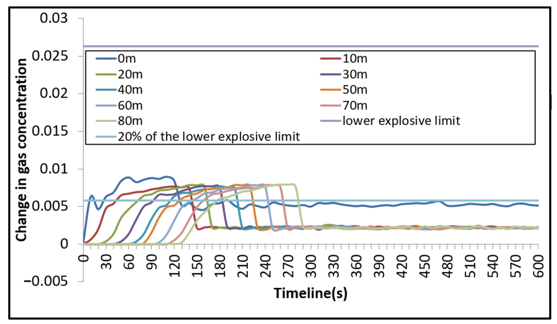
4.3. Early Warning Study of the Gas Cabin in Utility Tunnels

If the concentration of leaking gas in the gas cabin can be accurately obtained before a gas explosion occurs and early warning measures can be taken, it is likely that the accident damage can be effectively minimized. Turning on the fan in time can quickly reduce the concentration of gas in the cabin so that it is below 20 percent of the lower explosive limit and thus cannot reach explosive conditions. Proper gas sensor spacing will have a direct impact on when the explosion alarm is turned on. It further relates to the opening time of the fan, which ultimately results in different property or personnel damage. Therefore, it is necessary to first determine the appropriate fan rotation model and then analyze the appropriate sensor placement distance based on the gas leakage pattern.
At present, there are few documents on the distance requirements for sensor arrangement. As specified in the Technical Specification for Urban Integrated Pipe Corridor Project (GB50838-2015 [36]),and the Design Specification for Urban Gas (GB50028-2006 [37]), the integrated pipe corridor should be constructed simultaneously with firefighting, power supply, lighting, monitoring and alarm, ventilation, drainage, and marking facilities, but there is no detailed explanation for specific deployment. Natural gas pipeline compartments and compartments containing sewage pipes should have mechanical air intake and exhaust ventilation. Natural gas pipeline compartments should be ventilated not less than 6 times per hour for normal ventilation and not less than 12 times per hour for accident ventilation. If the concentration of natural gas in the cabin is greater than 20 percent of its lower explosive concentration value (volume fraction), the accident ventilation equipment of the accident section partition and its adjacent partition should be activated. As required in the document Petrochemical Flammable Gas and Toxic Gas Detection and Alarm Design Specification (GB50493-2009 [38]), when the detection (probe) test point is located on the upwind side of the minimum annual frequency wind direction of the release source, the distance between the detecting (probe) test point of the flammable gas body and the release source should not be greater than 15 m, and the detecting (probe) test device should not be greater than 7.5 m from any release source within its coverage. As mentioned in the Technical Standards for Urban Integrated Corridor Monitoring and Alarm System Engineering (GB51274-2017 [39]), the methane (CH4) sensor should not be more than 0.3 m from the top of the cabin, the hydrogen sulfide (H2S) sensor should be 0.3–0.6 m from the floor of the cabin, and the oxygen detection sensor should be 1.6–1.8 m from the floor of the cabin. In the gas cabin, two adjacent natural gas detectors should not be set up more than 15 m apart, and the installation should not be greater than 0.3 m from the top of the cabin. The primary alarm concentration setting of a natural gas alarm should not be greater than 20 percent of its lower explosive limit (volume fraction), and the secondary alarm concentration setting should not be greater than 40 percent of its lower explosive limit (volume fraction). When any one natural gas detector in the natural gas pipeline cabin exceeds the secondary alarm concentration setting value, the natural gas pipeline emergency shut-off valve linkage signal should be issued to close. In this paper, we will analyze the effect of ventilation under three different modes: natural ventilation, 6 times per hour, and 12 times per hour.
In order to obtain more scientific conclusions, this paper used the control variable method to study the gas evacuation effect under different fan operation modes. Therefore, when we studied the spacing of the natural gas sensor arrangement, we took a circular leak of 5 mm in diameter and conducted gas leak alarm analysis in a 200-m gas cabin. On observation line 1, sensors are installed at 0 m, 10 m, 20 m, 30 m, 40 m, 50 m, 60 m, 70 m, and 80 m from the leak hole and the primary alarm concentration is set at 20 percent of the lower gas explosion limit. When the sensor alarms sounds, the accident ventilation system for mechanical exhaust is opened and the gas concentration at various points in the compartment after the alarm sounds is analyzed.
As shown in Figure 15, the gas concentrations at different locations vary with time, but all show a gradual increase at first and then fluctuate up or down with time after stabilization. The gas concentration rises fastest above the leak hole (0 m). At approximately 6.7 s, its concentration reaches 20 percent of the lower explosive limit (mass fraction 0.00532452). At this point, the alarm sounded, the fan was turned on, and the air flow rate in the cabin became faster. The gas concentration at 0 m continued to increase and peaked at 0.00763541 after approximately 11.1 s. With the entry of natural air flow, the gas concentration at 0 m slowly decreases and finally fluctuates at approximately 20 percent of the lower explosive limit. At 10–70 m downstream of the observation line, the gas concentration starts to increase sequentially after 6.7 s and always fluctuates around 0.003989622.
As shown in Figure 16, when the gas sensor is installed 10 m away from the leak, the concentration at the sensor does not reach the alarm concentration until approximately 49.2 s. At this point, the fan starts to enter the accident ventilation mode and the gas concentration at 0 m starts to gradually decrease. The gas concentration at 10 m rises and then falls due to the jet principle.
As shown in Figure 17, when the gas sensor is installed 20 m away from the leak, the concentration at the sensor only reaches the alarm concentration at approximately 82.4 s. At this time, the fan turns on in accident ventilation mode and the gas concentration at 0 m begins to gradually decrease. The gas concentration at 10 m and 20 m increases and then decreases due to the jet principle. The gas concentration at 30 m gradually increases and reaches the highest peak value, then begins to decrease and finally remains at approximately 0.003989622.
Similarly, Figure 18, Figure 19, Figure 20, Figure 21 and Figure 22 show that the increased sensor spacing puts an increasing number of areas above the 20 percent risk of explosion lower limit. Therefore, if too few sensors are installed in the gas compartment, or if the spacing is too far apart, both will result in late detection of dangerous gas concentrations. The result was a late opening of the accident ventilation, which eventually led to a high concentration of leaking gas in the compartment, creating a significant safety hazard for the gas cabin.
If a sensor is installed at a distance of 0–80 m from the leak, once the sensor is triggered, the concentration rises rapidly at points downstream. The growth rate gradually slows down and finally reaches a certain peak and then begins to decline until it remains at approximately 0.003989622. This is due to the sensors being triggered in conjunction with the alarm going off and the cabin activating the accident ventilation system for 12 times per hour ventilation. The gas accumulated in the area from the leak to the sensor is carried downstream by the mechanical air flow, which accelerates the concentration increase in the downstream area. However, the amount of leaking gas in the interval from the leak to the sensor is constant, and the concentration of leaking gas downstream begins to decrease as the wind empties the area completely. As seen from the above group, whether the sensors are arranged 10 m, 20 m, or further apart, the gas concentration in the cabin will be higher than 20 percent of the lower explosion limit. Therefore, it is not feasible to use natural ventilation in the gas compartment of the integrated pipeline corridor, and when a leak occurs, it is difficult to quickly reduce the concentration of combustible gases in the compartment, even if the fan is turned on in time, which makes it prone to explosive accidents.
Subsequently, the case of gas leakage from a 5-mm diameter leak hole is used as a basis to study the effect of sensor spacing distance on the emergency response results when the gas cabin is under mechanical ventilation 6 times per hour. At this time, there are two main forms of gas in the gas cabin, natural ventilation and mechanical ventilation, and the gas flow rate in the cabin is a segmented function of time.
As shown in Figure 23, when the sensor is located directly above the leak, the gas concentration above the leak reaches 20 percent of the lower gas explosion limit at 4.8 s. The sensor triggers an alarm, which in turn turns on the fan’s accident ventilation mode, and the cabin is ventilated 12 times an hour. The maximum value of 0.00812 was obtained at 11.3 s directly above the observation point and then began to decrease gradually under the airflow, eventually converging to approximately 0.00526. These observations are below the lower limit of gas explosion concentration, and there is no possibility of an explosion. From 5.1 s onward, the gas concentration at the remaining points on observation line 1 gradually increases and finally stabilizes at approximately 0.00323, which is also below 20 percent of the lower explosive limit, with no possibility of explosion.
When the sensor is located 10 m below the leak, the concentration directly above the leak hole reaches 20 percent of the lower explosive limit at 11.5 s. At this time, the accident ventilation system is activated and the gas concentration directly above the leak hole is taken to a maximum value of 0.00803 at 51.6 s, followed by a gradual decrease under the effect of the jet of air and finally hovers at approximately 0.00529 (19.1 percent of the lower explosion limit). The gas concentration at the remaining points on the observation line start to change at 3.3 s and peak at 58.2 s, 59.5 s, 81.3 s, 103.5 s, 117.2 s, 133.3 s, 151.2 s, and 173.9 s, respectively, and fluctuate above and below 0.00228 after 220 s.
In the case of a gas sensor installed 20 m downstream, the concentration value at 10 m below the leak hole is greater than 20 percent of the lower gas explosion limit at 42.1–85.3 s. At 72.3–113.8 s, the concentration 20 m below the leak is greater than 20 percent of the lower limit of gas explosion. At 93.1–131.1 s, the concentration of gas 30 m below the leak should be greater than 20 percent of the lower limit of gas explosion. At 112.3–152.2 s, the concentration of gas 40 m below the leak should be greater than 20 percent of the lower limit of gas explosion. At 125.6–162.7 s, the gas concentration 50 m below the leak should be greater than 20 percent of the lower limit of gas explosion. At 148.3–184.6 s, the concentration of gas 60 m below the leak should be greater than 20 percent of the lower limit of gas explosion. At 159.5–200.3 s, the concentration of gas 70 m below the leak should be greater than 20 percent of the lower limit of gas explosion. At 179.4–224.3 s, the gas concentration 80 m below the leak should be greater than 20 percent of the lower limit of gas explosion. Taken together, the sensor captures the signal of abnormal gas concentration at 72.3 s and opens the accident ventilation system for the venting of gas in the compartment. However, at 42.1–224 s, the concentration of gas in many places is higher than the lower limit of gas explosion of 20 percent and the pipeline is extremely vulnerable to the risk of explosion when exposed to an open flame.
Similarly, Figure 24, Figure 25, Figure 26, Figure 27, Figure 28, Figure 29 and Figure 30 show that the concentration values at the points on the observation line change considerably as the installation distance of the gas sensors increases. Specifically, if the sensor is installed 10–30 m below the leakage outlet, the maximum concentration above the leakage outlet is taken at approximately 51 s. As the distance increases, it takes longer to reach the maximum concentration. However, the size of the peak does not change with the installation distance. As the distance between sensors increases, the time at risk increases, as shown in Table 3.
Therefore, when transporting natural gas in pipeline corridors, a gas sensor should be installed at least every 10 m and daily ventilation should be guaranteed 6 times per hour. The sensor alarm concentration should be set at 20 percent of the lower limit of gas explosion. When the concentration of gas in the cabin reaches this concentration, the alarm will be given and the accident ventilation mode will be activated to conduct ventilation at least 12 times per hour. The combination of normal ventilation and accident ventilation can ensure the cabin achieves scientific and effective prevention of gas leakage hazards.
Due to the different leak conditions, maintenance personnel need to adopt a targeted repair plan. When the concentration of leaking gas in the gas cabin is less than 20 percent of the lower explosive limit, maintenance workers can be dispatched directly into the cabin to weld the leak hole. When the gas concentration in the gas cabin is higher than 20 percent of the lower explosion limit, the fire doors at both ends of the leaking section should be closed immediately and mechanical ventilation should be used to reduce the gas concentration in the cabin. When the gas concentration drops below the safe level, repair workers can be dispatched to locate and repair the leaks.

5. Conclusions

Based on theoretical analysis and simulation software, this paper virtually modeled the entities in a utility tunnel in Beijing, simulated a gas pipeline leakage case, and obtained the gas leakage law. On this basis, the influence of the installation distance of the gas sensor on the ventilation effect was studied. The main conclusions of this paper include three aspects: leakage patterns, ventilation patterns, and sensor deployment methods, as shown below.
(1)
When gas leakage occurs from the gas pipeline of the utility tunnel, it is a dynamic process. Starting from 0 s, gas leaks from the hole and then peaks at 0.011989247 in a very short time. At 0–30 s, the peak value of gas leakage remains unchanged, and the leakage radius gradually increases. In addition, at 30–120 s, the gas concentration remains unchanged in two sections on the left and right sides of the leak. When the leakage time is within 0–80 s, the leakage law is symmetrical around the leakage point. However, after 80 s, the gas leakage law is no longer symmetrical around the leakage point. This is because the left side of the leak hole is closer to the air inlet and the right side is closer to the air outlet. The air flow will force the leaked gas to quickly gather downstream.
(2)
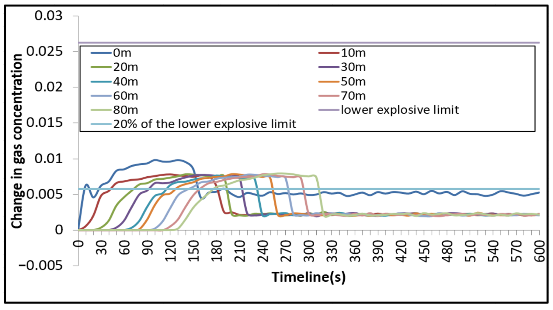
When the ventilation system of the gas cabin is natural ventilation without accidents, if a leakage accident occurs, even 12 ventilation operations per hour cannot guarantee that the gas concentration in the cabin is lower than 20 percent of the lower explosion limit. Therefore, the gas cabin must maintain daily mechanical ventilation at least 6 times per hour. This ventilation model has also become a more scientific and safe ventilation method for utility tunnels and provides a certain theoretical basis for the development of subsequent safety specifications.
(3)
Considering economic factors and ensuring that the ventilation system can effectively discharge the leaked gas out of the cabin in time, the optimal arrangement distance of the sensors in the gas cabin of the utility tunnel is approximately 10 m, and the sensor alarm concentration should be set to the gas explosion lower limit of 20 percent. By arranging sensors in the way of this paper, utility tunnel managers can maximize cost savings and avoid unnecessary waste while ensuring safety.
If the gas pipeline in the utility tunnel leaks, corresponding measures need to be taken in time to reduce disaster losses. When the leakage does not exceed 20 percent of the lower limit of the gas explosion, workers can be sent directly into the cabin to make repairs, such as welding. When the leakage is between the upper and lower limits of the gas explosion, it is necessary to turn off the gas source and turn on the emergency ventilation system to remove the gas. When the gas leakage exceeds the upper explosion limit, the high-concentration zone needs to be sealed off, and then inert gas should be injected to replace and discharge the leaked gas.

Author Contributions

Conceptualization, R.W., Z.Z. and D.G.; data curation, R.W. and Z.Z.; formal analysis, R.W.; investigation, D.G.; methodology, R.W.; writing—original draft, R.W.; writing—review and editing, R.W. All authors have read and agreed to the published version of the manuscript.

Funding

This research was funded by the Beijing Social Science Foundation, China, under grants 19JDGLA002 and 18JDGLA018, and the MOE (Ministry of Education in China) Project of Humanities and Social Sciences, under grant 19YJC630043.

Institutional Review Board Statement

Not applicable.

Informed Consent Statement

Not applicable.

Data Availability Statement

Some or all data, models, or code that support the findings of this study are available from the corresponding author upon reasonable request.

Acknowledgments

This work was supported by the Beijing Logistics Informatics Research Base. We appreciate their support very much.

Conflicts of Interest

The authors declare no conflict of interest.

References

  1. Canto-Perello, J.; Curiel-Esparza, J. Assessing governance issues of urban utility tunnels. Tunn. Undergr. Space Technol. 2013, 33, 82–87. [Google Scholar] [CrossRef]
  2. Cano-Hurtado, J.; Canto-Perello, J. Sustainable development of urban underground space for utilities. Tunn. Undergr. Space Technol. 1999, 14, 335–340. [Google Scholar] [CrossRef]
  3. Wang, T.Y.; Tan, L.X.; Xie, S.Y.; Ma, B.S. Development and applications of common utility tunnels in China. Tunn. Undergr. Space Technol. 2018, 76, 92–106. [Google Scholar] [CrossRef]
  4. Canto-Perello, J.; Curiel-Esparza, J.; Calvo, V. Strategic decision support system for utility tunnel’s planning applying A’WOT method. Tunn. Undergr. Space Technol. 2016, 55, 146–152. [Google Scholar] [CrossRef]
  5. Canto-Perello, J.; Curiel-Esparza, J. Risks and potential hazards in utility tunnels for urban areas. Proc. Inst. Civil Eng.-Munic. Eng. 2003, 156, 51–56. [Google Scholar] [CrossRef]
  6. Cai, Q.J.; Hu, Q.J.; Ma, G.L. Improved Hybrid Reasoning Approach to Safety Risk Perception under Uncertainty for Mountain Tunnel Construction. J. Constr. Eng. Manag. 2021, 147, 04021105. [Google Scholar] [CrossRef]
  7. Ma, L.; Bin Luo, H.; Chen, H.R. Safety risk analysis based on a geotechnical instrumentation data warehouse in metro tunnel project. Autom. Constr. 2013, 34, 75–84. [Google Scholar] [CrossRef]
  8. Zhang, G.D.; Shi, M.X. Bayesian assessment of utility tunnel risk based on information sharing mechanism. J. Intell. Fuzzy Syst. 2021, 41, 4749–4757. [Google Scholar] [CrossRef]
  9. Kim, Y.A.; Ryoo, B.Y.; Kim, Y.S.; Huh, W.C. Major Accident Factors for Effective Safety Management of Highway Construction Projects. J. Constr. Eng. Manag. 2013, 139, 628–640. [Google Scholar] [CrossRef]
  10. Jiang, Y.J.; Zhang, X.P.; Taniguchi, T. Quantitative condition inspection and assessment of tunnel lining. Autom. Constr. 2019, 102, 258–269. [Google Scholar] [CrossRef]
  11. Zhang, L.M.; Wu, X.G.; Liu, H.T. Strategies to Reduce Ground Settlement from Shallow Tunnel Excavation: A Case Study in China. J. Constr. Eng. Manag. 2016, 142, 04016001. [Google Scholar] [CrossRef]
  12. Liu, C.; AbouRizk, S.; Morley, D.; Lei, Z. Data-Driven Simulation-Based Analytics for Heavy Equipment Life-Cycle Cost. J. Constr. Eng. Manag. 2020, 146, 04020038. [Google Scholar] [CrossRef]
  13. Arabi, S.; Eshtehardian, E.; Shafiei, I. Using Bayesian Networks for Selecting Risk-Response Strategies in Construction Projects. J. Constr. Eng. Manag. 2022, 148, 04022067. [Google Scholar] [CrossRef]
  14. Pilao, R.; Ramalho, E.; Pinho, C. Explosibility of cork dust in methane/air mixtures. J. Loss Prev. Process Ind. 2006, 1, 17–23. [Google Scholar] [CrossRef]
  15. Bauwens, C.R.; Chaffee, J.; Dorofeev, S. Effect of ignition location, vent size and obstacles on vented explosion overpressures in propane-air mixtures. Combust. Sci. Technol. 2010, 182, 1915–1932. [Google Scholar] [CrossRef]
  16. Qian, H.M.; Li, J.; Zong, Z.H.; Wu, C.Q.; Pan, Y.H. Behavior of precast segmental utility tunnel under ground surface Explosion: A numerical study. Tunn. Undergr. Space Technol. 2021, 115, 104071. [Google Scholar] [CrossRef]
  17. Fan, C.G.; Chen, J.; Zhou, Y.; Liu, X.P. Effects of fire location on the capacity of smoke exhaust from natural ventilation shafts in urban tunnels. Fire Mater. 2018, 42, 974–984. [Google Scholar] [CrossRef]
  18. Yang, C.; Peng, F.L. Discussion on the development of underground utility tunnels in China. Procedia Eng. 2016, 165, 540–548. [Google Scholar] [CrossRef]
  19. Li, P.F.; Xu, M.Y.; Wang, F.F. Proficient in CFD Engineering Simulation and Case Study; The Posts and Telecommunications Press: Beijing, China, 2011; ISBN 9787115260802. [Google Scholar]
  20. Al-Bataineh, M.; AbouRizk, S.; Parkis, H. Using Simulation to Plan Tunnel Construction. J. Constr. Eng. Manag. 2013, 139, 564–571. [Google Scholar] [CrossRef]
  21. Yan, Q.S.; Zhang, Y.N.; Sun, Q.W. Characteristic Study on Gas Blast Loadings in an Urban Utility Tunnel. J. Perform. Constr. Facil. 2020, 34, 04020076. [Google Scholar] [CrossRef]
  22. Ouyang, M.; Liu, C.; Wu, S.Y. Worst-case vulnerability assessment and mitigation model of urban utility tunnels. Reliab. Eng. Syst. Saf. 2020, 197, 106856. [Google Scholar] [CrossRef]
  23. Lin, Z.Z.; Guo, C.C.; Ni, P.P.; Cao, D.F.; Huang, L.; Guo, Z.F.; Dong, P. Experimental and numerical investigations into leakage behaviour of a novel prefabricated utility tunnel. Tunn. Undergr. Space Technol. 2020, 104, 103529. [Google Scholar] [CrossRef]
  24. Yin, Z.Y.; Wang, P.; Zhang, F.S. Effect of particle shape on the progressive failure of shield tunnel face in granular soils by coupled FDM-DEM method. Tunn. Undergr. Space Technol. 2020, 100, 103394. [Google Scholar] [CrossRef]
  25. Wang, P.; Karatza, Z.; Arson, C. DEM modelling of sequential fragmentation of zeolite granules under oedometric compression based on XCT observations. Powder Technol. 2019, 347, 66–75. [Google Scholar] [CrossRef]
  26. Zhang, H.T.; Zhao, Y.F. Study on Underground Utility Tunnel Fire Characteristics under Sealing and Ventilation Conditions. Adv. Civ. Eng. 2020, 2020, 9128704. [Google Scholar] [CrossRef]
  27. Mi, H.F.; Liu, Y.L.; Jiao, Z.R.; Wang, W.H.; Wang, Q.S. A numerical study on the optimization of ventilation mode during emergency of cable fire in utility tunnel. Tunn. Undergr. Space Technol. 2020, 100, 103403. [Google Scholar] [CrossRef]
  28. Tang, G.Y.; Fang, Y.M.; Zhong, Y.; Yuan, J.; Ruan, B.; Fang, Y.; Wu, Q. Numerical Study on the Longitudinal Response Characteristics of Utility Tunnel under Strong Earthquake: A Case Study. Adv. Civ. Eng. 2020, 2020, 8813303. [Google Scholar] [CrossRef]
  29. Yang, Y.M.; Li, Z.G.; Li, Y.Q.; Xu, R.; Wang, Y.K. Research on the anti-seismic performance of composite precast utility tunnels based on the shaking table test and simulation analysis. Comput. Concr. 2021, 27, 163–173. [Google Scholar]
  30. Wang, W.H.; Zhu, Z.X.; Jiao, Z.R.; Mi, H.F.; Wang, Q.S. Characteristics of fire and smoke in the natural gas cabin of urban underground utility tunnels based on CFD simulations. Tunn. Undergr. Space Technol. 2021, 109, 103748. [Google Scholar] [CrossRef]
  31. Zhao, Y.C.; Zhu, G.Q.; Gao, Y.J. Experimental study on smoke temperature distribution under different power conditions in utility tunnel. Case Stud. Therm. Eng. 2018, 12, 69–76. [Google Scholar]
  32. Bu, F.X.; Liu, Y.; Wang, Z.X.; Xu, Z.; Chen, S.Q.; Hao, G.W.; Guan, B. Analysis of natural gas leakage diffusion characteristics and prediction of invasion distance in utility tunnels. J. Nat. Gas Sci. Eng. 2021, 96, 104270. [Google Scholar] [CrossRef]
  33. Kunii, D.; Levenspiel, O. Fluidization Engineering; Butterworth-Heinemann: Boston, MA, USA, 1962; ISBN 0409902330. [Google Scholar]
  34. Montiel, H.; Vilchez, J.A.; Casal, J.; Arnaldos, J. Mathematical modeling of accidental gas release. J. Hazard. Mater. 1998, 59, 211–233. [Google Scholar] [CrossRef]
  35. Woodward, J.L.; Mudan, K.S. Liquid and gas discharge rates through holes in process vessels. J. Loss Prev. Proc. 1991, 4, 161–165. [Google Scholar] [CrossRef]
  36. GB50838-2015; Technical Specification for Urban Utility Tunnel Engineering. Standardization Administration of the People’s Republic of China: Beijing, China, 2015.
  37. GB/T50028-2006; Code for design of city gas engineering. Standardization Administration of the People’s Republic of China: Beijing, China, 2006.
  38. GB50493-2009; Specification for Design of Combustible Gas and Toxic Gas Detection and Alarm for Petrochemical Industry. Standardization Administration of the People’s Republic of China: Beijing, China, 2009.
  39. GB51274-2017; Technical Standard for Monitoring and Alarm System Engineering for Urban Utility Tunnel Engineering. Standardization Administration of the People’s Republic of China: Beijing, China, 2017.
Figure 1. Cross-sectional diagram of the Beijing Winter Olympic Games utility tunnel.
Sustainability 15 15375 g001
Figure 2. Position diagram of the gas pipeline and cabin.
Sustainability 15 15375 g002
Figure 3. Model drawing of the gas cabin section.
Sustainability 15 15375 g003
Figure 4. Schematic diagram of the leak model.
Sustainability 15 15375 g004
Figure 5. Schematic diagram of the gas cabin.
Sustainability 15 15375 g005
Figure 6. Grid encryption diagram of the gas leakage model.
Sustainability 15 15375 g006
Figure 7. Graph of gas leakage of observation Line 1 at 5–120 s.
Sustainability 15 15375 g007
Figure 8. Graph of gas leakage of observation Line 1 at 160–440 s.
Sustainability 15 15375 g008
Figure 9. Graph of gas leakage of observation Line 1 at 480–760 s.
Sustainability 15 15375 g009
Figure 10. Graph of gas leakage of observation line 2 at 5–120 s.
Sustainability 15 15375 g010
Figure 11. Graph of gas leakage of observation line 2 at 160–440 s.
Sustainability 15 15375 g011
Figure 12. Graph of gas leakage of observation line 2 at 480–760 s.
Sustainability 15 15375 g012
Figure 13. Diagram of the change in leakage radius of observation line 1 and observation line 2.
Sustainability 15 15375 g013
Figure 14. Diagram of the effect of leak-hole diameter on the diffusion radius.
Sustainability 15 15375 g014
Figure 15. Diagram of gas sensors installed at 0 m from the leak.
Sustainability 15 15375 g015
Figure 16. Diagram of gas sensors installed 10 m from the leak.
Sustainability 15 15375 g016
Figure 17. Diagram of gas sensors installed 20 m from the leak.
Sustainability 15 15375 g017
Figure 18. Diagram of gas sensors installed 30 m from the leak.
Sustainability 15 15375 g018
Figure 19. Diagram of gas sensors installed 40 m from the leak.
Sustainability 15 15375 g019
Figure 20. Diagram of gas sensors installed 50 m from the leak.
Sustainability 15 15375 g020
Figure 21. Diagram of gas sensors installed 60 m from the leak.
Sustainability 15 15375 g021
Figure 22. Diagram of gas sensors installed 70 m from the leak.
Sustainability 15 15375 g022
Figure 23. Diagram of gas sensors installed 0 m from the leak.
Sustainability 15 15375 g023
Figure 24. Diagram of gas sensors installed 10 m from the leak.
Sustainability 15 15375 g024
Figure 25. Diagram of gas sensors installed 20 m from the leak.
Sustainability 15 15375 g025
Figure 26. Diagram of gas sensors installed 30 m from the leak.
Sustainability 15 15375 g026
Figure 27. Diagram of gas sensors installed 40 m from the leak.
Sustainability 15 15375 g027
Figure 28. Diagram of gas sensors installed 50 m from the leak.
Sustainability 15 15375 g028
Figure 29. Diagram of gas sensors installed 60 m from the leak.
Sustainability 15 15375 g029
Figure 30. Diagram of gas sensors installed 70 m from the leak.
Sustainability 15 15375 g030
Table 1. Grid irrelevance verification table.
Number of Grids (Ten Thousands)Measurement
Point 1
Measurement
Point 2
Measurement
Point 3
Measurement Point 4Measurement Point 5
3000.000326546480.000305456120.000291235650.000288040320.00028013151
3500.000401256420.000392541850.0003945178910.000395689220.00038421638
4000.000423564180.000412874590.0004114287130.000412844630.00040924677
4500.000455328910.000446123850.0004401368280.000431362370.00043017865
5000.000472418950.000452794320.0004596379250.000455166730.00044372919
5500.000421559740.000430908720.0004135332870.000419875610.00040765612
6000.000413264980.000421156590.0004097946520.000403316450.00039532316
6500.000395613650.000400216480.0004021649560.000392314920.00038398422
7000.000387652960.000393165180.0003923264620.000384698790.00038203126
7500.000037453480.000364942370.0003579569630.000346598910.00034377918
Table 2. Boundary condition setting table.
No.Setting BoundariesBoundary ConditionsParameter Setting
1Leak portEntrance of mass outflowTemperature, Mass flow, Pressure
2FansInlet of pressureTemperature, Wind speed, Ventilation type, Ventilation Time interval, Air pressure
3Air outlet mezzanineOutlet of pressureStatic pressure, Temperature
4Pipe wall and inside pipe cabinSurface boundaryTemperature difference between tube wall and cabin wall, Thermal conductivity, Material type
Table 3. Diagram of the sensor installation position in relation to the moment of danger.
Installation Location (t)Starting Moment (s)Unwinding Time (s)Time Interval (s)
0 m000
10 m000
20 m72.3224.4152.1
30 m43.2257.1213.9
40 m44.5276.3231.8
50 m45.1287.5242.4
60 m45.8303.7257.9
70 m46.2314.5268.3
Disclaimer/Publisher’s Note: The statements, opinions and data contained in all publications are solely those of the individual author(s) and contributor(s) and not of MDPI and/or the editor(s). MDPI and/or the editor(s) disclaim responsibility for any injury to people or property resulting from any ideas, methods, instructions or products referred to in the content.

