
Forecasting Accuracy of Traditional Regression, Machine Learning, and Deep Learning: A Study of Environmental Emissions in Saudi Arabia


Abstract
:
1. Introduction
2. Literature Review
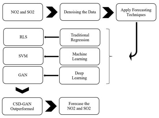
3. Methodology and Data Setting
3.1. Denoising Methods
- The sparse or approximation sparse representation for the signal may be written as if the signal is sparse under an orthogonal basis.
- We created an dimensional observation matrix to quantify the sparse coefficients s and produced an observation vector, . The transformed basis is unaffected by this observation matrix . The whole sensing procedure is as follows:
- After receiving the compressed sensed signal , the recovery of from is carried out as follows:
3.2. Artificial Intelligence (AI)
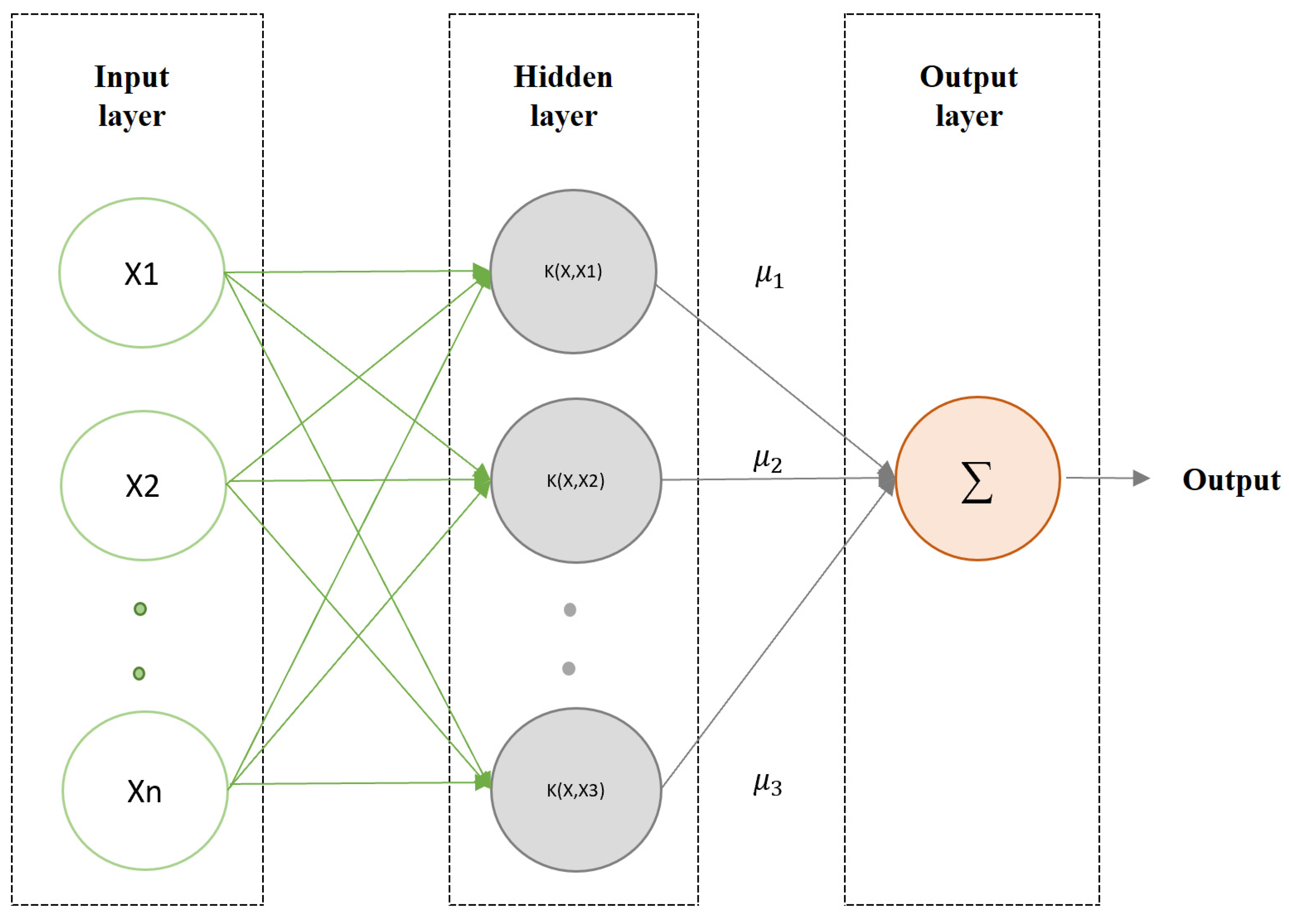
3.2.1. Least Squares Support Vector Regression
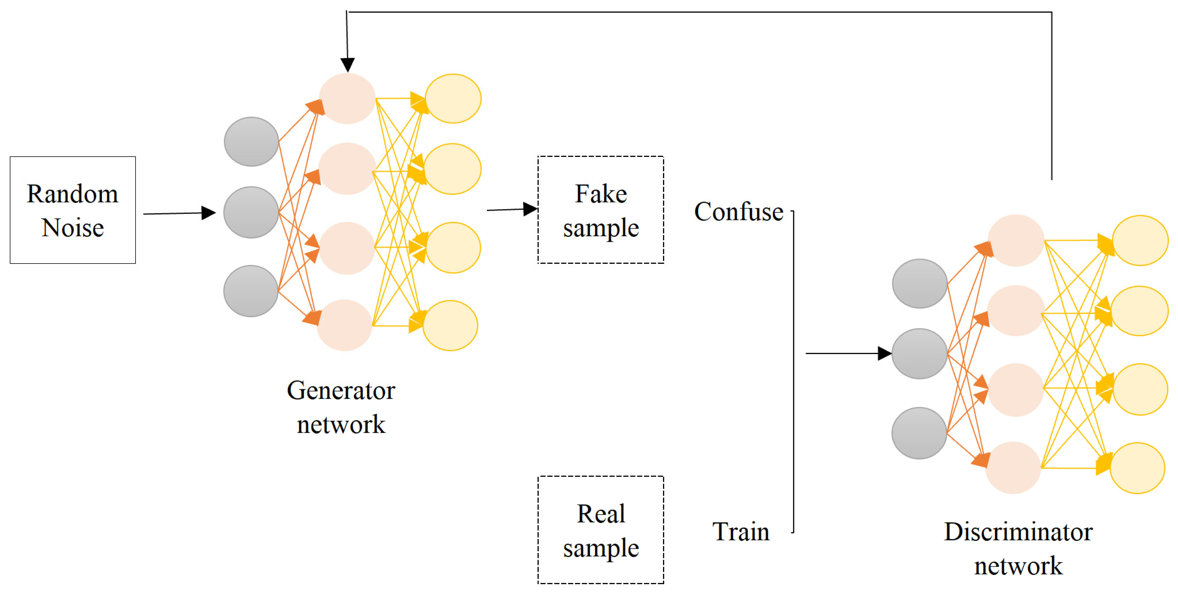
3.2.2. Generative Adversarial Network (GAN)
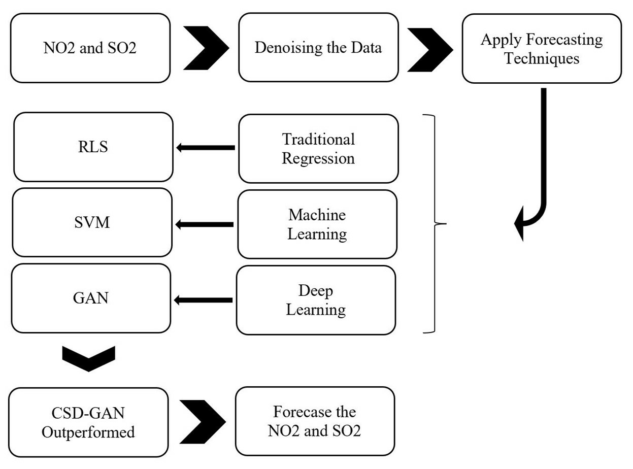
3.3. AI Forecasted Models Integrated with Compressed Sensing-Based Denoising (CSD-AI)
- The original data comprises a trend , and noise is first represented by an appropriate transform basis; in our instance, a wavelet basis. The sparse coefficients are then sampled using a Gaussian white noise sampling matrix. Ultimately, the cleaned data may be obtained via the OMP recovery process for more research.
- After data denoising, a powerful AI approach, such as an SVM or ANN, is used to model the cleaned data and make predictions for the original .
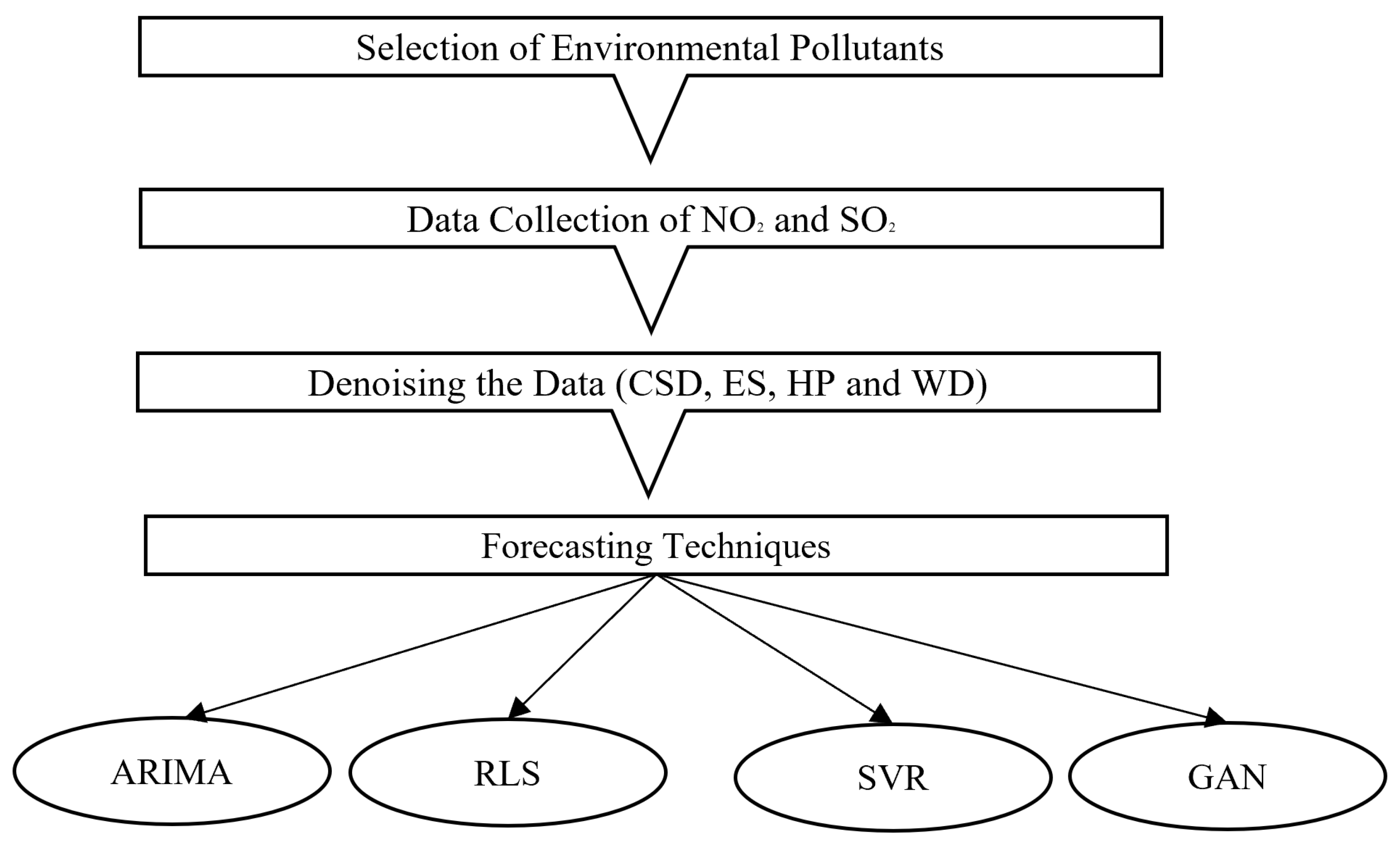
3.4. Data Description
3.5. Performance Evaluation Criteria
3.6. Benchmark Models
3.7. Parameter Settings
4. Results and Discussion
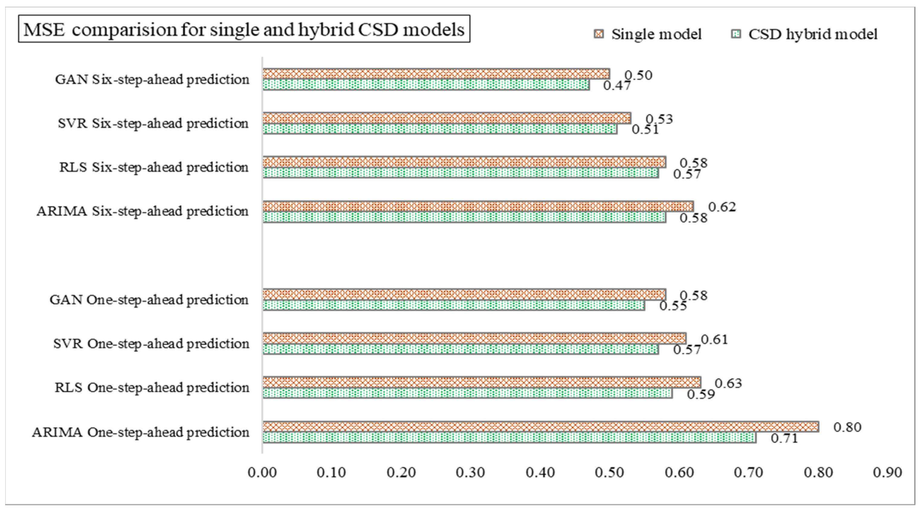
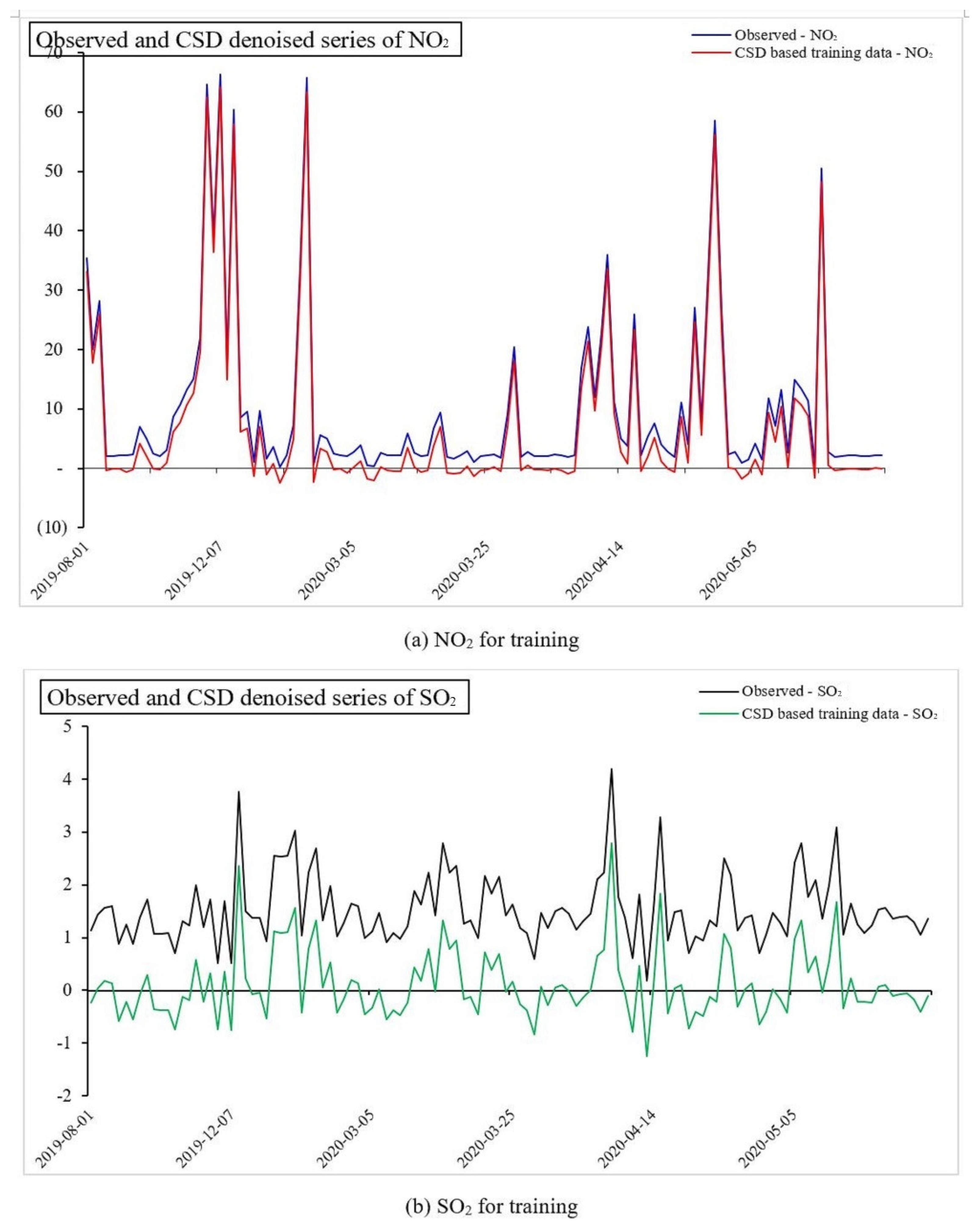
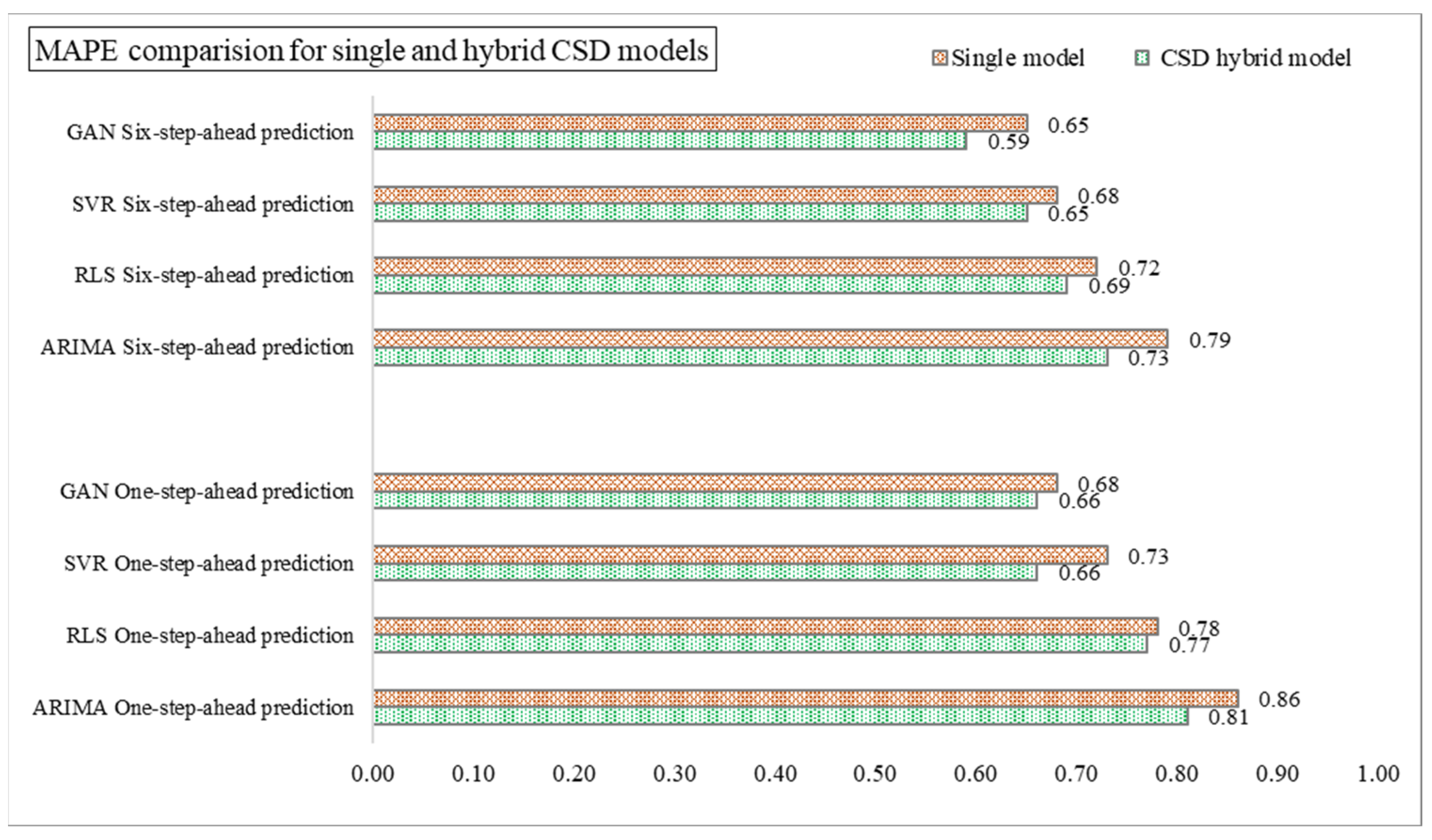
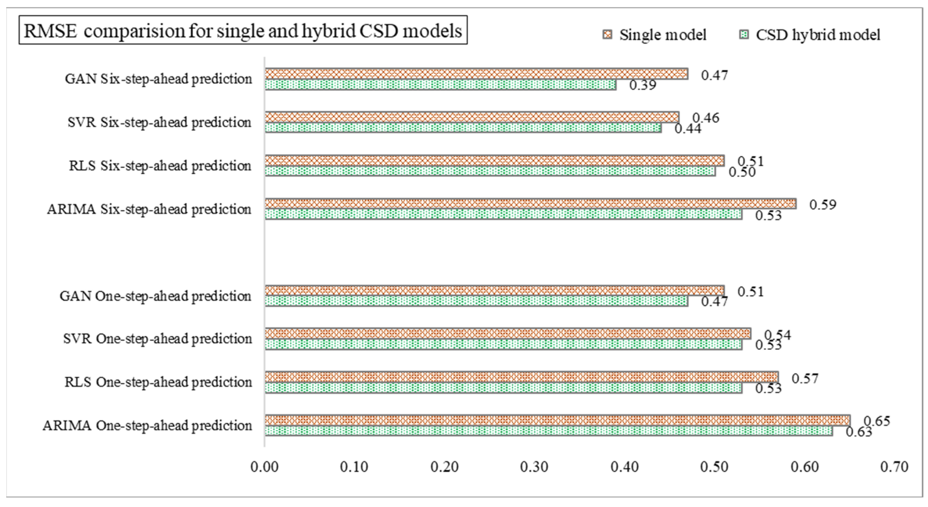
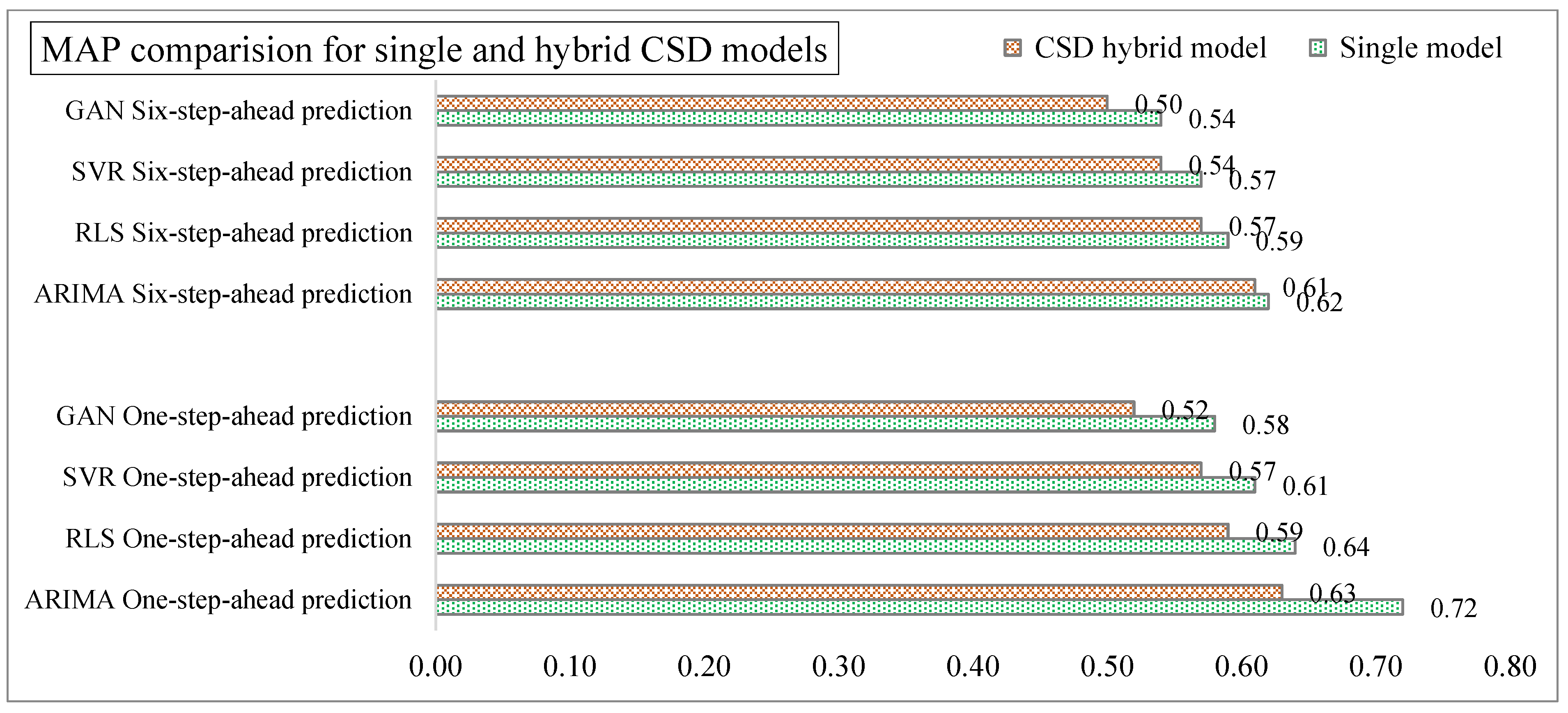
4.1. Implementation of CSD-Based Models in Forecasting (Effectiveness of CSD in Forecasting)
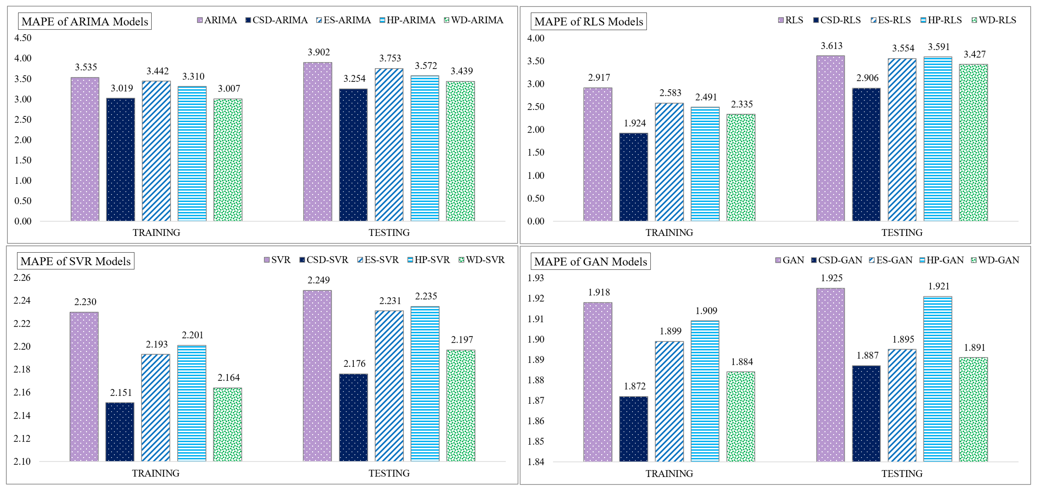
4.2. Performance of CSD-Based Denoising Methods
4.3. Diebold–Mariano (DM) Forecast Accuracy Test
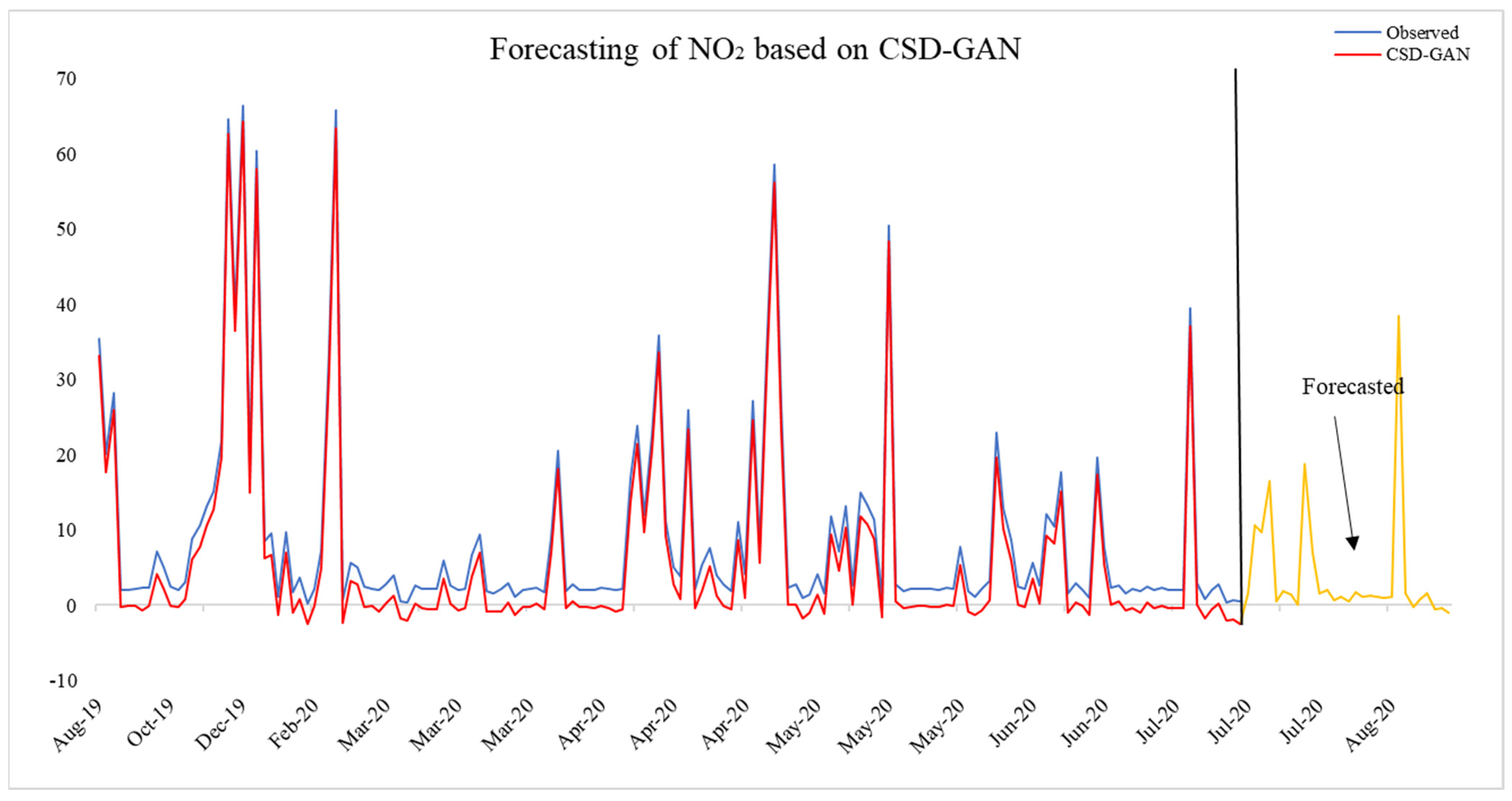
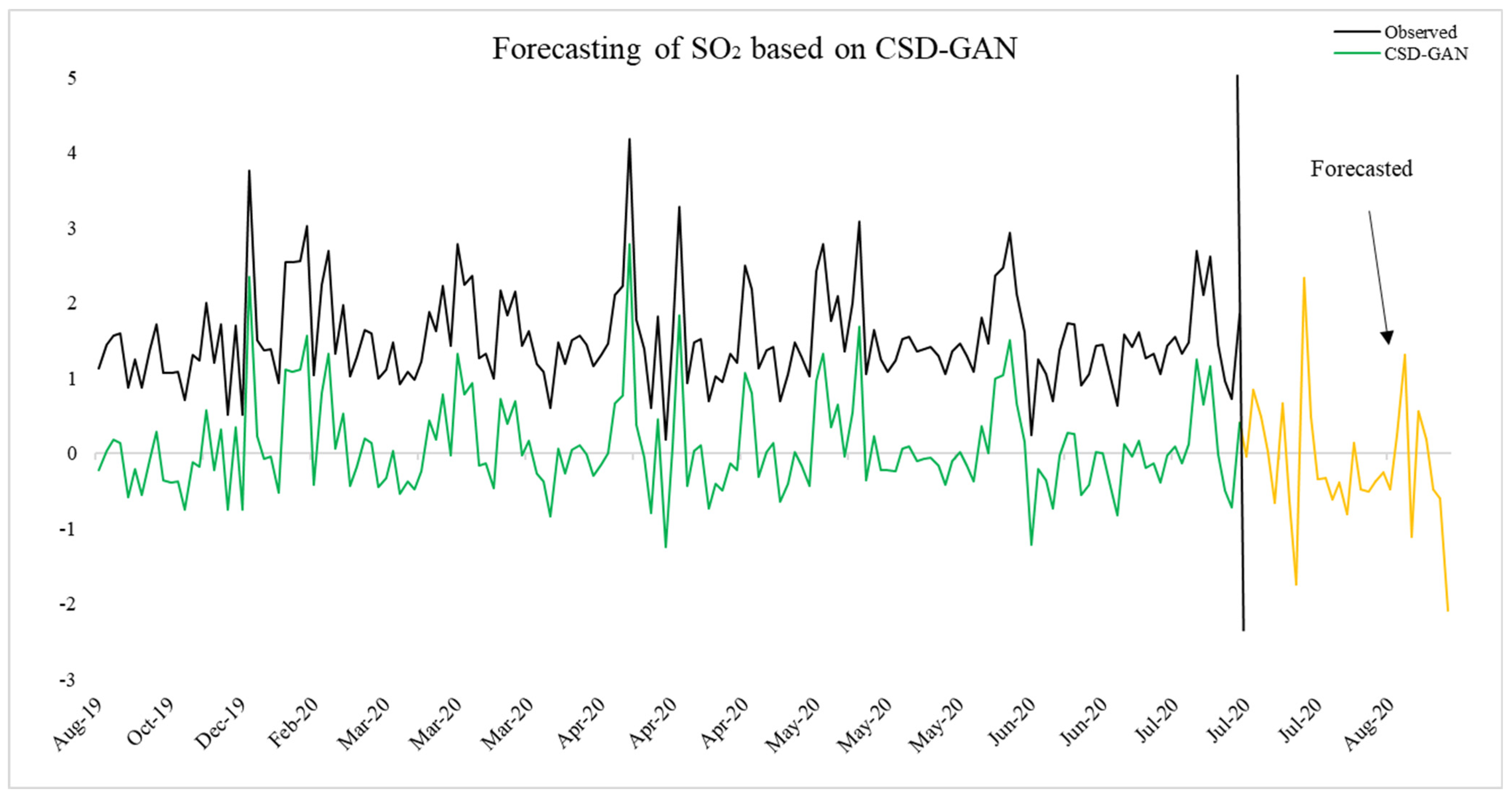
4.4. CSD-GAN-Based Out-of Sample Forecasting of NO2 and SO2
4.5. Discussion and Summarizations
5. Conclusions
Author Contributions
Funding
Institutional Review Board Statement
Informed Consent Statement
Data Availability Statement
Conflicts of Interest
References
- Singh, R.L.; Singh, P.K. Global Environmental Problems. In Principles and Applications of Environmental Biotechnology for a Sustainable Future; Springer: Singapore, 2016; pp. 13–41. [Google Scholar] [CrossRef]
- Baklanov, A.; Molina, L.T.; Gauss, M. Megacities, Air Quality and Climate. Atmos. Environ. 2016, 126, 235–249. [Google Scholar] [CrossRef]
- Moore, M.; Gould, P.; Keary, B.S. Global Urbanization and Impact on Health. Int. J. Hyg. Environ. Health 2003, 206, 269–278. [Google Scholar] [CrossRef]
- Pinault, L.; Crouse, D.; Jerrett, M.; Brauer, M.; Tjepkema, M. Spatial Associations between Socioeconomic Groups and NO2 Air Pollution Exposure within Three Large Canadian Cities. Environ. Res. 2016, 147, 373–382. [Google Scholar] [CrossRef]
- Sonibare, J.A.; Akeredolu, F.A. A Theoretical Prediction of Non-Methane Gaseous Emissions from Natural Gas Combustion. Energy Policy 2004, 32, 1653–1665. [Google Scholar] [CrossRef]
- Turias, I.J.; González, F.J.; Martin, M.L.; Galindo, P.L. Prediction Models of CO, SPM and SO2 Concentrations in the Campo de Gibraltar Region, Spain: A Multiple Comparison Strategy. Environ. Monit. Assess. 2008, 143, 131–146. [Google Scholar] [CrossRef]
- Wang, P.; Zhang, H.; Qin, Z.; Zhang, G. A Novel Hybrid-Garch Model Based on ARIMA and SVM for PM2.5 Concentrations Forecasting. Atmos. Pollut. Res. 2017, 8, 850–860. [Google Scholar] [CrossRef]
- Pandey, J.S.; Kumar, R.; Devotta, S. Health Risks of NO2, SPM and SO2 in Delhi (India). Atmos. Environ. 2005, 39, 6868–6874. [Google Scholar] [CrossRef]
- McKendry, I.G. Evaluation of Artificial Neural Networks for Fine Particulate Pollution (PM10 and PM2.5) Forecasting. J. Air Waste Manag. Assoc. 2002, 52, 1096–1101. [Google Scholar] [CrossRef]
- Dutta, A.; Jinsart, W. Air Pollution in Indian Cities and Comparison of MLR, ANN and CART Models for Predicting PM10 Concentrations in Guwahati, India. Asian J. Atmos. Environ. 2021, 15, 1–26. [Google Scholar] [CrossRef]
- Shang, Z.; He, J. Predicting Hourly PM2.5 Concentrations Based on Random Forest and Ensemble Neural Network. In Proceedings of the 2018 Chinese Automation Congress (CAC), Xi’an, China, 30 November–2 December 2018; pp. 2341–2345. [Google Scholar] [CrossRef]
- Bozdağ, A.; Dokuz, Y.; Gökçek, Ö.B. Spatial Prediction of PM10 Concentration Using Machine Learning Algorithms in Ankara, Turkey. Environ. Pollut. 2020, 263, 114635. [Google Scholar] [CrossRef]
- Tripathi, A.K.; Sharma, K.; Bala, M. A Novel Clustering Method Using Enhanced Grey Wolf Optimizer and MapReduce. Big Data Res. 2018, 14, 93–100. [Google Scholar] [CrossRef]
- Wang, P.; Liu, Y.; Qin, Z.; Zhang, G. A Novel Hybrid Forecasting Model for PM10 and SO2 Daily Concentrations. Sci. Total Environ. 2015, 505, 1202–1212. [Google Scholar] [CrossRef]
- Wang, J.; Bai, L.; Wang, S.; Wang, C. Research and Application of the Hybrid Forecasting Model Based on Secondary Denoising and Multi-Objective Optimization for Air Pollution Early Warning System. J. Clean. Prod. 2019, 234, 54–70. [Google Scholar] [CrossRef]
- Sang, Y.F.; Wang, D.; Wu, J.C.; Zhu, Q.P.; Wang, L. Entropy-Based Wavelet de-Noising Method for Time Series Analysis. Entropy 2009, 11, 1123–1147. [Google Scholar] [CrossRef]
- Niu, L.; Shi, Y. A Hybrid Slantlet Denoising Least Squares Support Vector Regression Model for Exchange Rate Prediction. Procedia Comput. Sci. 2010, 1, 2397–2405. [Google Scholar] [CrossRef]
- de Faria, E.L.; Albuquerque, M.P.; Gonzalez, J.L.; Cavalcante, J.T.P.; Albuquerque, M.P. Predicting the Brazilian Stock Market through Neural Networks and Adaptive Exponential Smoothing Methods. Expert Syst. Appl. 2009, 36, 12506–12509. [Google Scholar] [CrossRef]
- Yuan, C. Forecasting Exchange Rates: The Multi-State Markov-Switching Model with Smoothing. Int. Rev. Econ. Financ. 2011, 20, 342–362. [Google Scholar] [CrossRef]
- Nasseri, M.; Moeini, A.; Tabesh, M. Forecasting Monthly Urban Water Demand Using Extended Kalman Filter and Genetic Programming. Expert Syst. Appl. 2011, 38, 7387–7395. [Google Scholar] [CrossRef]
- Chen, B.T.; Chen, M.Y.; Fan, M.H.; Chen, C.C. Forecasting Stock Price Based on Fuzzy Time-Series with Equal-Frequency Partitioning and Fast Fourier Transform Algorithm. In Proceedings of the 2012 Computing, Communications and Applications Conference, Hong Kong, China, 1–13 January 2012; pp. 238–243. [Google Scholar] [CrossRef]
- He, K.; Lai, K.K.; Xiang, G. Portfolio Value at Risk Estimate for Crude Oil Markets: A Multivariatewavelet Denoising Approach. Energies 2012, 5, 1018–1043. [Google Scholar] [CrossRef]
- Sang, Y.F. Improved Wavelet Modeling Framework for Hydrologic Time Series Forecasting. Water Resour. Manag. 2013, 27, 2807–2821. [Google Scholar] [CrossRef]
- Gardner, E.S. Exponential Smoothing: The State of the Art. J. Forecast. 1985, 4, 1–28. [Google Scholar] [CrossRef]
- Hodrick, R.J.; Prescott, E.C. Postwar U.S. Business Cycles: An Empirical Investigation; Ohio State University Press: Columbus, OH, USA, 1997; Volume 29, pp. 1–16. Available online: http://www.jstor.org/stable/2953682 (accessed on 5 February 2023).
- Kalman, R.E. A New Approach to Linear Filtering and Prediction Problems. J. Fluids Eng. Trans. ASME 1960, 82, 35–45. [Google Scholar] [CrossRef]
- Ahmed, N.; Natarajan, T.; Rao, K.R. Discrete Cosine Transform. IEEE Trans. Comput. 1974, 100, 90–93. [Google Scholar] [CrossRef]
- Mallat, S.G. A Theory for Multiresolution Signal Decomposition: The Wavelet Representation. IEEE Trans. Pattern Anal. Mach. Intell. 1989, 11, 79–85. [Google Scholar] [CrossRef]
- Zhu, L.; Zhu, Y.; Mao, H.; Gu, M. A New Method for Sparse Signal Denoising Based on Compressed Sensing. In Proceedings of the 2009 Second International Symposium on Knowledge Acquisition and Modeling, Wuhan, China, 30 November–1 December 2009; pp. 35–38. [Google Scholar] [CrossRef]
- Han, B.; Xiong, J.; Li, L.; Yang, J.; Wang, Z. Research on Millimeter-Wave Image Denoising Method Based on Contourlet and Compressed Sensing. In Proceedings of the 2010 2nd International Conference on Signal Processing Systems, Dalian, China, 5–7 July 2010. [Google Scholar]
- Sharma, A.; Massey, D.D.; Taneja, A. A Study of Horizontal Distribution Pattern of Particulate and Gaseous Pollutants Based on Ambient Monitoring near a Busy Highway. Urban Clim. 2018, 24, 643–656. [Google Scholar] [CrossRef]
- Li, R.; Cui, L.; Liang, J.; Zhao, Y.; Zhang, Z.; Fu, H. Estimating Historical SO2 Level across the Whole China during 1973–2014 Using Random Forest Model. Chemosphere 2020, 247, 125839. [Google Scholar] [CrossRef]
- Sheng, T.; Pan, J.; Duan, Y.; Liu, Q.; Fu, Q. Study on Characteristics of Typical Traffic Environment Air Pollution in Shanghai. China Environ. Sci. 2019, 39, 3193–3200. [Google Scholar]
- Wu, L.; Noels, L. Recurrent Neural Networks (RNNs) with Dimensionality Reduction and Break down in Computational Mechanics; Application to Multi-Scale Localization Step. Comput. Methods Appl. Mech. Eng. 2022, 390, 114476. [Google Scholar] [CrossRef]
- Wu, C.-L.; He, H.-D.; Song, R.-F.; Peng, Z.-R. Prediction of Air Pollutants on Roadside of the Elevated Roads with Combination of Pollutants Periodicity and Deep Learning Method. Build. Environ. 2022, 207, 108436. [Google Scholar] [CrossRef]
- Du, W.; Chen, L.; Wang, H.; Shan, Z.; Zhou, Z.; Li, W.; Wang, Y. Deciphering Urban Traffic Impacts on Air Quality by Deep Learning and Emission Inventory. J. Environ. Sci. 2023, 124, 745–757. [Google Scholar] [CrossRef]
- Kurnaz, G.; Demir, A.S. Prediction of SO2 and PM10 Air Pollutants Using a Deep Learning-Based Recurrent Neural Network: Case of Industrial City Sakarya. Urban Clim. 2022, 41, 101051. [Google Scholar] [CrossRef]
- Aceves-Fernández, M.A.; Domínguez-Guevara, R.; Pedraza-Ortega, J.C.; Vargas-Soto, J.E. Evaluation of Key Parameters Using Deep Convolutional Neural Networks for Airborne Pollution (PM10) Prediction. Discret. Dyn. Nat. Soc. 2020, 2020, 2792481. [Google Scholar] [CrossRef]
- Atamaleki, A.; Motesaddi Zarandi, S.; Fakhri, Y.; Abouee Mehrizi, E.; Hesam, G.; Faramarzi, M.; Darbandi, M. Estimation of Air Pollutants Emission (PM10, CO, SO2 and NOx) during Development of the Industry Using AUSTAL 2000 Model: A New Method for Sustainable Development. MethodsX 2019, 6, 1581–1590. [Google Scholar] [CrossRef] [PubMed]
- Perez, P.; Menares, C.; Ramírez, C. PM2.5 Forecasting in Coyhaique, the Most Polluted City in the Americas. Urban Clim. 2020, 32, 100608. [Google Scholar] [CrossRef]
- Janarthanan, R.; Partheeban, P.; Somasundaram, K.; Navin Elamparithi, P. A Deep Learning Approach for Prediction of Air Quality Index in a Metropolitan City. Sustain. Cities Soc. 2021, 67, 102720. [Google Scholar] [CrossRef]
- Al-Janabi, S.; Mohammad, M.; Al-Sultan, A. A New Method for Prediction of Air Pollution Based on Intelligent Computation. Soft Comput. 2020, 24, 661–680. [Google Scholar] [CrossRef]
- Al Dakheel, J.; Del Pero, C.; Aste, N.; Leonforte, F. Smart Buildings Features and Key Performance Indicators: A Review. Sustain. Cities Soc. 2020, 61, 102328. [Google Scholar] [CrossRef]
- Aggarwal, A.; Toshniwal, D. A Hybrid Deep Learning Framework for Urban Air Quality Forecasting. J. Clean. Prod. 2021, 329, 129660. [Google Scholar] [CrossRef]
- Chiang, P.W.; Horng, S.J. Hybrid Time-Series Framework for Daily-Based PM2.5 Forecasting. IEEE Access 2021, 9, 104162–104176. [Google Scholar] [CrossRef]
- Du, S.; Li, T.; Yang, Y.; Horng, S.J. Multivariate Time Series Forecasting via Attention-Based Encoder–Decoder Framework. Neurocomputing 2020, 388, 269–279. [Google Scholar] [CrossRef]
- Du, S.; Li, T.; Gong, X.; Horng, S.J. A Hybrid Method for Traffic Flow Forecasting Using Multimodal Deep Learning. Int. J. Comput. Intell. Syst. 2020, 13, 85–97. [Google Scholar] [CrossRef]
- Du, S.; Li, T.; Yang, Y.; Horng, S.J. Deep Air Quality Forecasting Using Hybrid Deep Learning Framework. IEEE Trans. Knowl. Data Eng. 2021, 33, 2412–2424. [Google Scholar] [CrossRef]
- Elder, Y.; Kutyniok, G. Compressed Sensing (Theory and Applications); Cambridge University Press: Cambridge, UK, 2012. [Google Scholar]
- Vapnik, V.N. The Nature of Statistical Learning Theory; Springer: New York, NY, USA, 2000. [Google Scholar] [CrossRef]
- Yin, T.; Wang, Y. Predicting the Price of WTI Crude Oil Futures Using Artificial Intelligence Model with Chaos. Fuel 2022, 316, 122523. [Google Scholar] [CrossRef]
- Broock, W.A.; Scheinkman, J.A.; Dechert, W.D.; LeBaron, B. A Test for Independence Based on the Correlation Dimension. Econom. Rev. 1996, 15, 197–235. [Google Scholar] [CrossRef]
- Zagajewski, B.; Kluczek, M.; Raczko, E.; Njegovec, A.; Dabija, A.; Kycko, M. Comparison of Random Forest, Support Vector Machines, and Neural Networks for Post-Disaster Forest Species Mapping of the Krkonoše/Karkonosze Transboundary Biosphere Reserve. Remote Sens. 2021, 13, 2581. [Google Scholar] [CrossRef]
- Dou, Z.; Sun, Y.; Zhu, J.; Zhou, Z. The Evaluation Prediction System for Urban Advanced Manufacturing Development. Systems 2023, 11, 392. [Google Scholar] [CrossRef]
- Yang, X.; Tan, L.; He, L. A Robust Least Squares Support Vector Machine for Regression and Classification with Noise. Neurocomputing 2014, 140, 41–52. [Google Scholar] [CrossRef]
- Balabin, R.M.; Lomakina, E.I. Support Vector Machine Regression (SVR/LS-SVM)—An Alternative to Neural Networks (ANN) for Analytical Chemistry? Comparison of Nonlinear Methods on near Infrared (NIR) Spectroscopy Data. Analyst 2011, 136, 1703–1712. [Google Scholar] [CrossRef]
- Aggarwal, A.; Mittal, M.; Battineni, G. Generative Adversarial Network: An Overview of Theory and Applications. Int. J. Inf. Manag. Data Insights 2021, 1, 100004. [Google Scholar] [CrossRef]
- Sahoo, L.; Praharaj, B.B.; Sahoo, M.K. Air Quality Prediction Using Artificial Neural Network. Adv. Intell. Syst. Comput. 2021, 1248, 31–37. [Google Scholar] [CrossRef]
- Shams, S.R.; Jahani, A.; Kalantary, S.; Moeinaddini, M.; Khorasani, N. The Evaluation on Artificial Neural Networks (ANN) and Multiple Linear Regressions (MLR) Models for Predicting SO2 Concentration. Urban Clim. 2021, 37, 100837. [Google Scholar] [CrossRef]
- Bowerman, B.L.; O’Connell, R.T.; Koehler, A.B. Forecasting, Time Series, and Regression: An Applied Approach; Thomson Brooks/Cole Publishing: Pacific Grove, CA, USA, 2005. [Google Scholar]
- Baxter, M.; King, R.G. Approximate Band-Pass Filters for Economic Time Series. NBER Work. Pap. Ser. 1995, 5022, 1–53. [Google Scholar]
- Stoffer, D.S.; Shumway, R.H. An Approach to Time Series Smoothing and Forecasting Using the EM Algorithm. J. Time Ser. Anal. 1982, 3, 253–264. [Google Scholar]
- Struzik, Z.R. Wavelet Methods in (Financial) Time-Series Processing. Phys. A Stat. Mech. Its Appl. 2001, 296, 307–319. [Google Scholar] [CrossRef]
- Donoho, D.L. De-Noising by Modified Soft-Thresholding. IEEE Asia-Pacific Conf. Circuits Syst.-Proc. 2000, 41, 760–762. [Google Scholar] [CrossRef]
- Diebold, F.; Mariano, R. Comparing Predictive Accuracy. J. Bus. Econ. Stat. 1995, 13, 253–263. [Google Scholar]
- Hornik, K.; Stinchcombe, M.; White, H. Presentation on Multilayer Feedforward Networks Are Universal Approximators; Elsevier: Amsterdam, The Netherlands, 1989. [Google Scholar]
- Harvey, D.; Leybourne, S.; Newbold, P. Testing the Equality of Prediction Mean Squared Errors. Int. J. Forecast. 1997, 13, 281–291. [Google Scholar] [CrossRef]
- Yu, L.; Zhao, Y.; Tang, L. A Compressed Sensing Based AI Learning Paradigm for Crude Oil Price Forecasting. Energy Econ. 2014, 46, 236–245. [Google Scholar] [CrossRef]


| Section A: Descriptive | NO2 | SO2 |
| Mean | 3.974 | 1.528 |
| Maximum | 6.370 | 4.190 |
| Minimum | 0.200 | 0.190 |
| Std. Dev. | 0.388 | 0.635 |
| Skewness | 1.640 | 1.181 |
| Kurtosis | 10.070 | 5.218 |
| Jarque–Bera | 519.074 | 70.012 |
| Probability | 0.000 | 0.000 |
| ARCH-LM | 89.261 *** | 210.674 *** |
| Section B: BDS | ||
| 2 | 0.352 *** | 0.140 *** |
| 3 | 0.394 *** | 0.189 *** |
| 4 | 0.410 *** | 0.200 *** |
| 5 | 0.573 *** | 0.342 *** |
| 6 | 0.499 *** | 0.418 *** |
| ARIMA | CSD-ARIMA | ES-ARIMA | HP-ARIMA | WD-ARIMA | ||
|---|---|---|---|---|---|---|
| MAPE | Training data | 3.535 | 3.019 | 3.442 | 3.310 | 3.007 |
| Testing data | 3.902 | 3.254 | 3.753 | 3.572 | 3.439 | |
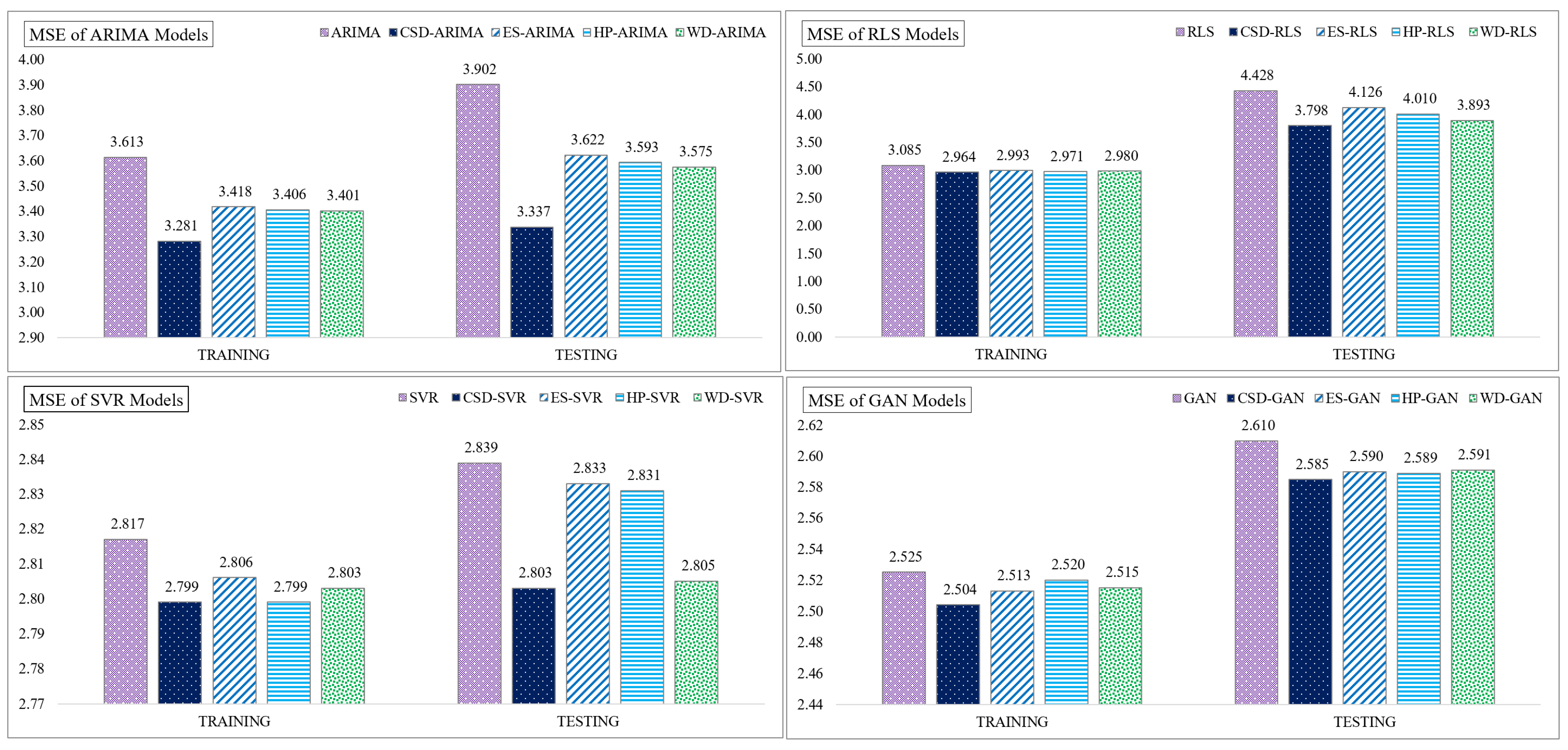
| MSE | Training data | 3.613 | 3.281 | 3.418 | 3.406 | 3.401 |
| Testing data | 3.902 | 3.337 | 3.622 | 3.593 | 3.575 | |
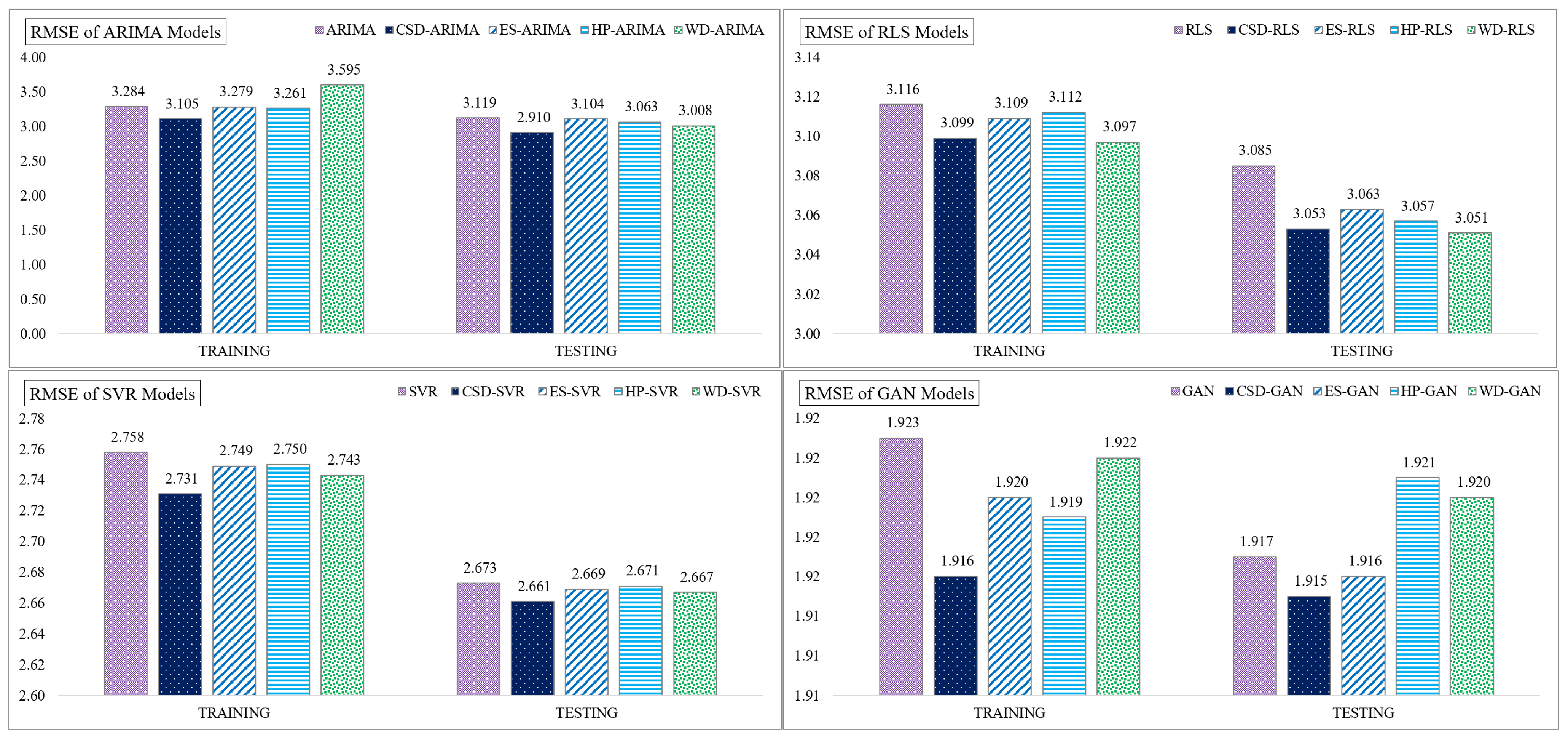
| RMSE | Training data | 3.284 | 3.105 | 3.279 | 3.261 | 3.595 |
| Testing data | 3.119 | 2.910 | 3.104 | 3.063 | 3.008 | |
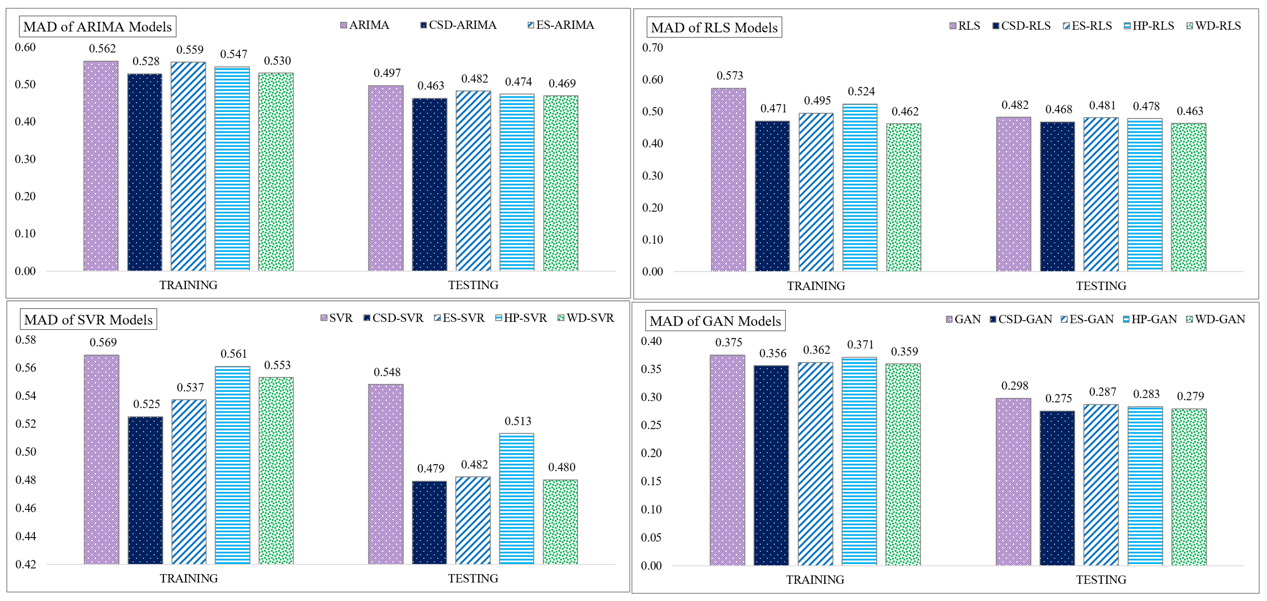
| MAD | Training data | 0.562 | 0.528 | 0.559 | 0.547 | 0.530 |
| Testing data | 0.497 | 0.463 | 0.482 | 0.474 | 0.469 | |
| RLS | CSD-RLS | ES-RLS | HP-RLS | WD-RLS | ||
| MAPE | Training data | 2.917 | 1.924 | 2.583 | 2.491 | 2.335 |
| Testing data | 3.613 | 2.906 | 3.554 | 3.591 | 3.427 | |
| MSE | Training data | 3.085 | 2.964 | 2.993 | 2.971 | 2.980 |
| Testing data | 4.428 | 3.798 | 4.126 | 4.010 | 3.893 | |
| RMSE | Training data | 3.116 | 3.099 | 3.109 | 3.112 | 3.097 |
| Testing data | 3.085 | 3.053 | 3.063 | 3.057 | 3.051 | |
| MAD | Training data | 0.573 | 0.471 | 0.495 | 0.524 | 0.462 |
| Testing data | 0.482 | 0.468 | 0.481 | 0.478 | 0.463 | |
| SVR | CSD-SVR | ES-SVR | HP-SVR | WD-SVR | ||
| MAPE | Training data | 2.230 | 2.151 | 2.193 | 2.201 | 2.164 |
| Testing data | 2.249 | 2.176 | 2.231 | 2.235 | 2.197 | |
| MSE | Training data | 2.817 | 2.799 | 2.806 | 2.799 | 2.803 |
| Testing data | 2.839 | 2.803 | 2.833 | 2.831 | 2.805 | |
| RMSE | Training data | 2.758 | 2.731 | 2.749 | 2.750 | 2.743 |
| Testing data | 2.673 | 2.661 | 2.669 | 2.671 | 2.667 | |
| MAD | Training data | 0.569 | 0.525 | 0.537 | 0.561 | 0.553 |
| Testing data | 0.548 | 0.479 | 0.482 | 0.513 | 0.480 | |
| GAN | CSD-GAN | ES-GAN | HP-GAN | WD-GAN | ||
| MAPE | Training data | 1.918 | 1.872 | 1.899 | 1.909 | 1.884 |
| Testing data | 1.925 | 1.887 | 1.895 | 1.921 | 1.891 | |
| MSE | Training data | 2.525 | 2.504 | 2.513 | 2.520 | 2.515 |
| Testing data | 2.610 | 2.585 | 2.590 | 2.589 | 2.591 | |
| RMSE | Training data | 1.923 | 1.916 | 1.920 | 1.919 | 1.922 |
| Testing data | 1.917 | 1.915 | 1.916 | 1.921 | 1.920 | |
| MAD | Training data | 0.375 | 0.356 | 0.362 | 0.371 | 0.359 |
| Testing data | 0.298 | 0.275 | 0.287 | 0.283 | 0.279 |
| MSE | ARIMA | RLS | SVR | GAN | CSD-ARIMA | CSD-RLS | CSD-SVR |
|---|---|---|---|---|---|---|---|
| S0 | −71.102 | −63.824 | −21.453 | −49.822 | −57.285 | −44.101 | −75.086 |
| P0 | 0.000 | 0.000 | 0.000 | 0.000 | 0.000 | 0.000 | 0.000 |
| Result | Reject H0; Accept H1 | ||||||
Disclaimer/Publisher’s Note: The statements, opinions and data contained in all publications are solely those of the individual author(s) and contributor(s) and not of MDPI and/or the editor(s). MDPI and/or the editor(s) disclaim responsibility for any injury to people or property resulting from any ideas, methods, instructions or products referred to in the content. |
© 2023 by the authors. Licensee MDPI, Basel, Switzerland. This article is an open access article distributed under the terms and conditions of the Creative Commons Attribution (CC BY) license (https://creativecommons.org/licenses/by/4.0/).
Share and Cite
Sarwar, S.; Aziz, G.; Balsalobre-Lorente, D. Forecasting Accuracy of Traditional Regression, Machine Learning, and Deep Learning: A Study of Environmental Emissions in Saudi Arabia. Sustainability 2023, 15, 14957. https://doi.org/10.3390/su152014957
Sarwar S, Aziz G, Balsalobre-Lorente D. Forecasting Accuracy of Traditional Regression, Machine Learning, and Deep Learning: A Study of Environmental Emissions in Saudi Arabia. Sustainability. 2023; 15(20):14957. https://doi.org/10.3390/su152014957
Chicago/Turabian StyleSarwar, Suleman, Ghazala Aziz, and Daniel Balsalobre-Lorente. 2023. "Forecasting Accuracy of Traditional Regression, Machine Learning, and Deep Learning: A Study of Environmental Emissions in Saudi Arabia" Sustainability 15, no. 20: 14957. https://doi.org/10.3390/su152014957
APA StyleSarwar, S., Aziz, G., & Balsalobre-Lorente, D. (2023). Forecasting Accuracy of Traditional Regression, Machine Learning, and Deep Learning: A Study of Environmental Emissions in Saudi Arabia. Sustainability, 15(20), 14957. https://doi.org/10.3390/su152014957