Article

Research on Transportation Carbon Emission Peak Prediction and Judgment System in China

1
College of Transportation, Shandong University of Science and Technology, Qingdao 266590, China
2
International Cooperation Center of National Development and Reform Commission, Beijing 100038, China
*
Author to whom correspondence should be addressed.
Sustainability 2023, 15(20), 14880; https://doi.org/10.3390/su152014880
Submission received: 29 August 2023 / Revised: 28 September 2023 / Accepted: 10 October 2023 / Published: 15 October 2023

Abstract

:
The transportation sector is a major contributor to carbon emissions, and managing its carbon peak is essential for China to reach the 2030 carbon peak target. This paper uses the autoregressive integrated moving average model (ARIMA) to design baseline scenarios and “double carbon” scenarios (carbon peak and carbon neutrality) based on the accounting of transportation carbon emissions in 30 provinces and cities in China to facilitate regional differentiation and forecast the development trend of transportation carbon emissions. Using the fuzzy comprehensive evaluation method, a comprehensive transportation carbon emission research and judgment system has been developed based on the forecast results. The research indicates a substantial increase in carbon dioxide (CO2) emissions from transport in China over the past 15 years, with an average growth rate of 5.9%, from 387.42 mt in 2005 to 917.00 mt in 2019. In the scenario prediction analysis, the overall carbon emission of the “two-carbon” scenario exhibits varying levels of reduction compared with the baseline scenario. According to the comprehensive research and judgment system, when the comprehensive evaluation index corresponding to the turning point year of transportation carbon emissions is greater than 0.85, and the index remains above 0.85 after the turning point, it can be judged that a region has achieved the peak of transportation carbon dioxide emissions under 95% possibility. It shows that Chinas policies and strategies for carbon and emission reduction have played a significant role in transportation, but the low-carbon transformation and development still face great challenges.

1. Introduction

Climate change caused by greenhouse gas emissions has become the focus of global attention. China attaches great importance to climate change [1]. On 27 October 2021, China issued a white paper entitled “Chinese Policies and Actions to Address Climate Change”, which introduced China’s progress in addressing climate change, shared practices and experience in handling climate change, and helped the Paris Agreement achieve stability. Its primary contents include that it is a significant decision of China to achieve carbon peaking and carbon neutrality and that, at the same time, China faces the severe challenge of emission reduction to achieve peak carbon at a lower peak value and achieve carbon neutrality within the specified time. Transportation is one of the crucial sources of carbon emissions. The International Road Federation (IRF) estimates that by 2050, the energy consumption related to transportation will increase by 21 percent to 25 percent compared with 2016. The carbon peaking and carbon neutrality goal has pressured the transportation field tremendously. Still, it can promote the “high-quality” development of the economy, enhance the voice of global environmental issues, and have economic and political significance for China [2].
Carbon emission reduction (CER) in transportation means “decoupling” transportation development from carbon emissions [3]. Transportation is one of the critical industries of energy consumption and direct carbon emissions. From the perspective of the current law of economic and social development, the development of transportation has a significantly positive correlation with the modernization process and the improvement of living standards. Regions with the highest TCE are developed economies and some emerging economies. China is in the process of rapid industrialization, urbanization, and motorization. In the future, the resource occupation and total CO2 emissions in the transportation field will show a gradual increase. It is also a great challenge to achieve comprehensive “decoupling”. Accelerating the carbon peaking and carbon neutralization from intensity to the total amount and conducting carbon emission measurement analysis and emission reduction path research have important practical significance for building a low-carbon economic system.
Publicity and Education Center of the Ministry of Ecology and Environment, School of Applied Economics at the Renmin University of China, and Didi Development Research Institute jointly released the “Digital Travel Helps Carbon Neutrality” research report. The report says that compared with other industries, it is more challenging to achieve the carbon peaking and carbon neutrality goals in the transportation industry [4]. Continuous breakthroughs should be made in the top-level design, road space layout, slow traffic system construction, automobile electrification transformation, green low-carbon technology, etc. In addition, promoting the realization of the carbon peaking and carbon neutrality goal is the “main theme” in the transportation field during the 14th Five Year Plan period. Different from developed countries, China’s realization of the carbon peaking and carbon neutrality goal refers to effective emission reduction in the context of ensuring sustainable economic and social development, helping to achieve the transition from the “high growth” model to the “high quality” model. In transportation, the realization of a “carbon peak” means that the development of transportation is not restricted, but the task of reaching the peak within the specified time and keeping the “low peak” as far as possible is completed. The carbon peaking and carbon neutrality goal is an essential challenge for industry development, and China has implemented a series of strategies, measures, and actions in this regard.
The transportation field holds immense promise in terms of reducing carbon emissions and emissions [5]. Accurately grasping the trend of carbon peaking in China’s transportation, constructing a quantified comprehensive judgment system for carbon peaking, and determining the research and judgment standards for carbon peaking are vital to the next low-carbon development planning of China’s transportation industry and the adjustment and formulation of carbon peaking strategies. Simultaneously, it would serve as a benchmark and roadmap for numerous nations that have yet to reach the peak transport carbon, further propelling the attainment of the worldwide carbon dioxide emissions peak and establishing the groundwork for the accomplishment of the global carbon-neutral objective.

2. Literature Review

2.1. Research on Carbon Peaking

In the face of increasingly severe global climate and environmental change, research on carbon emission peak path, time, and future climate simulation has become a focus in low-carbon economics. Many studies estimate national and regional CO2 emissions, providing a scientific perspective for future sustainable development strategies. Prasad and Raturi [6] use the LEAP model to study the greenhouse gas emissions of Fiji’s road transport from 2016 to 2040. Selvakkumaran and Limmeechokchai [7] have built an AIM/Enduse model to study the carbon emissions of Thailand’s transportation industry. Gao and Pan [8] studied the carbon peak by establishing a dynamic model of economy-energy-carbon emission in Shanghai. Zhang and Luo [9] used the LEAP model to predict peak carbon emissions. Capros et al. [10] used the PRIMES model to assess decarbonization in the EU in 2030 under the “Clean Energy for All Europeans” package.

2.2. Research on Transportation Carbon Emission Prediction

The most widely used carbon emission prediction is scenario prediction of the future trend of carbon emissions. Liimatainen et al. [11] have created six scenarios based on the forecast of seven indicators of CO2 emissions from Finnish freight transport, and the results show that the average annual emission reduction in 2030 will be more than 26%. Dhar et al. [12] have used the ANSWER MARKAL model to compare and analyze four possible transport (passenger and freight) carbon emission scenarios for India spanning till 2050. Wang et al. [13] have quantitatively simulated the emission reduction effects of different policy measures under different scenarios, such as optimization of transportation structure, application of energy-saving and emission-reduction technologies, and new energy vehicles. AlSabbagh et al. [14] analyze the CO2 emission scenario of Bahrain’s road passenger transport sector. Wang et al. [15] analyze China’s road transport industry’s CO2 emission reduction scenario.
Scholars have also used many other methods to predict carbon emissions. Gao and Sun [16] use the grey relational analysis model to investigate the evolutionary relationship of TCE and relevant factors in Jilin Province. Wu et al. [17] combine the Logarithmic Mean Divisia Index (LMDI) model with the Tapio decoupling model, predict and analyze the time, path, and quality of carbon peaking in the transportation industry in China and its eastern, central, and western regions. Byers et al. [18] have studied and analyzed the low-carbon development measures of the UK transport system from 2010 to 2050 by building a practical energy analysis framework for future transport routes. By creating a C3IAM/NET transport model, Tang et al. [19] have simulated the CER potential of intercity passenger transport by adjusting the transport structure, improving energy efficiency, and promoting alternative fuels. They predicted that China’s intercity passenger transport would peak in 2030. Fernández-Dacosta et al. [20] compare the potential of carbon intensity reduction of different alternative fuels. Zhou et al. [21] have studied the CO2 emission performance of the transportation field in 30 administrative regions of China using the output-oriented data envelopment analysis model with different returns to scale.

2.3. Research on Influencing Factors of Transportation Carbon Emission

Identifying the influencing factors of transportation carbon emissions is the basic work of formulating policies and measures for the development of low-carbon transportation. Wang et al. [3] have used the generalized division index method (GDIM) to analyze influencing factors and decoupling Elasticity of Chinese TCE. Talbi [22] uses the vector autoregression (VAR) model to analyze the influencing factors of the change of CO2 emissions in Tunisia’s transport sector from 1980 to 2014, including economic growth, urbanization rate, energy intensity, and other factors. Mattioli [23] has studied the development of low-carbon transportation from the social equity perspective. Fan and Lei [24] studied the effects of energy structure, energy intensity, output value per unit traffic turnover, traffic intensity, economic growth, and population size on carbon emissions in Beijing’s transportation sector between 1995 and 2012, taking into account the extended Kaya identity. Xu and Lin [25] contend that urbanization has a considerable effect on CO2 emissions in the transportation industry. Tsita and Pilavachi [26] used long-term range energy alternatives planning (LEAP) to forecast CO2 emissions from the Greek transport sector for 2010–2050 based on various scenarios utilizing alternative technologies. The evidence suggests that advances in technology are essential for preserving energy and decreasing emissions. Zhang et al. [27] hold the belief that the construction of infrastructure is crucial in the reduction of carbon. Chen et al. [28] used GDIM, Tapio, and scenario-based dynamic forecasting methods to study the drivers of carbon emissions change in China’s transportation from 2005–2019 and concluded that investment is the main driver of carbon emissions growth in the transportation industry. Wang et al. [29] analyzed the factors affecting the carbon emissions of the railway transportation industry in BRIC nations and determined that the economic output effect factors contributed positively to the increase of carbon emissions in all the identified countries.
After reviewing both domestic and international research, it is evident that when it comes to transportation, academics concentrate on forecasting and evaluating the factors that contribute to carbon emission, and the scenario analysis model has become a popular tool in the transportation sector. Despite this, further research is needed to explore the prevalence of carbon peaking between provinces and cities, with the majority of studies concentrating on large or densely populated areas such as countries or megacities. Subsequently, there is still a dearth of studies that take into account the viewpoint of provinces and cities that have successfully reached carbon peaking, particularly in the absence of research on the process of carbon peaking. The current research does not have a benchmark to determine if carbon dioxide emissions have reached their highest point in forecasting or analysis.
Therefore, the innovation of this paper lies in its utilization of a fuzzy comprehensive evaluation approach to build a thorough assessment system for quantified carbon emission peaks, assess the carbon peak condition of Chinese provinces and cities, and create a comprehensive evaluation system for carbon emission peak that is appropriate for China and other provinces and cities. This research rectifies the deficiencies of existing studies in the area of carbon dioxide emission peak assessment and furnishes effective policy recommendations for achieving China’s carbon peak.

3. Methodology and Data

3.1. Methodology

3.1.1. ARIMA Model

TCE data are a non-stationary series, also known as weak stationarity, characterized by dependence, i.e., the value of a specific time in the future depends on its past information. The ARIMA model is a time series and prediction method [30]. Its basic principle is first to use the d-order difference to stabilize the non-stationary time series and then use Autoregressive AR(p), Moving Average MA(q), Autocorrelation Function (ACF), and Partial Correlation Coefficient (PCF) to identify the model for the stabilized time series. This model is often used for time series analysis.
First, the primary variables involved in the formula are described. X t is a time series, x t represents the t-th point in the time series (t is an integer from 1 to N), and N represents the length of the series. In this model, relevant variables are shown in Table 1.
Secondly, the stationarity of the time series X t is tested. Generally, ACF and PACF functions are used to judge the type. For ACF, the calculation formula is as follows.
The correlation coefficient ACF (unbiased) is as follows:
a c f k = r k = c k c 0 = N N k × t = k + 1 N ( x t μ ) ( x t k μ ) t = 1 N x t μ 2
The correlation coefficient ACF (biased) is as follows:
a c f k = r k = c k c 0 = N N k × t = k + 1 N ( x t μ ) ( x t k μ ) t = 1 N x t μ 2
For PACF, the calculation process is more complex, and the following assumptions are generally made first:
x i + 1 = 1 x i + 2 x i 1 + + k x i k + 1 + δ i + 1
In this formula, j ( j   i s   a n   i n t e g e r   f r o m   1   t o   K ) is the linear correlation coefficient, δ i + 1 is noise, i.e., we assume that the point x i + 1 is linearly related to the first k points, as follows x i k 1 , x i k + 2 , , x i . PACF represents the correlation between x i and x i k . Therefore, the PACF formula of the sequence is as follows:
p a c f k = k
The solution process of k is omitted here, which can be determined by programming.
If the time series X t fails to pass the stationarity test, the original data must be stabilized and transformed into a weakly stationary series by difference. In practical application, d is usually equal to 1 or 2, and the determination method is that the data pass the stationarity test after d-order difference. ARMA(p, q) model has many identification methods, but it is generally identified by autocorrelation coefficient (ACF) and partial correlation coefficient (PCF). If the d-order difference of X t is a stable ARIMA process, it is called the autoregressive moving average summation model. The solution formula of d is as follows:
W t = ( 1 B ) d X t
If W t follows A R M A ( p , q ) model, X t is said to be an A R I M A ( p , d , q ) process.
ARIMA includes three components: autoregressive, differential, and moving average. p, d, and q represent autoregressive order (Lags of time series data used in the prediction model, also called AR/Auto Recursive term.), difference number (How many orders of real-time data need to be differentiated to obtain stable data, also called Integrated term.), and moving average order (Lags of prediction error used in the prediction model, also called MA/Moving Average.), respectively, and the Bayesian Information Criterion (BIC) can be used to calculate the BIC value to select p value and q value.
Bayesian decision theory is a part of BIC. It means that under incomplete reporting, some unknown states are estimated with subjective probability, and then the occurrence probability is modified with the Bayesian formula. Finally, the expected value and the modified possibility are used to make the optimal decision, with the formula as follows:
B I C = ln N h 2 l n ( L )
where h is the number of model parameters, and h = 5 is taken in this paper. L is the likelihood function and ln N h is the penalty term. When the dimension is too large, and the training sample data are small, dimension disaster can be effectively avoided. The order of the optimal A R I M A ( p , d , q ) model is the p-value, and q-value that minimizes the BIC value.
For the time series that have passed the stationarity test, the stationary process W t can be used to replace the position of the unstable X t in the ARIMA model, namely:
W t = c + ϕ 1 W t 1 + + ϕ p W t p + ε t + θ t ε t 1 + θ q ε t q
Represented by the lag operator:
Φ B W t = c + Θ ( B ) ε t
where, { ε t } is a white noise process,
Φ B = 1 ϕ 1 B ϕ 2 B 2 ϕ q B q
Θ B = 1 + θ 1 B + θ 2 B 2 + + θ q B q
A R M A ( p , q ) model after the d-order difference change is called A R I M A ( p , d , q ) model. Equation (15) is equivalent to the following equation:
Φ B ( 1 B ) d X t = c + Θ ( B ) ε t
Finally, the A R I M A ( p , d , q ) that has been established is used to predict the changes of subsequent index values, and the final prediction results are obtained. ARIMA model is suitable for short-term prediction. In this paper, an adaptive method is proposed to predict carbon emissions in the field of transportation by using JupyterLab 3.0 software.

3.1.2. Fuzzy Comprehensive Evaluation Method

The concept of fuzzy set theory was put forward by the American automatic control expert Zadeh in 1965 to express the uncertainty of things, which is an important part of fuzzy mathematics and the theoretical source of fuzzy comprehensive evaluation and analysis [31].
The fuzzy comprehensive evaluation method blurs all aspects and factors of the evaluation object and then gets the final evaluation result through the fuzzy comprehensive operation. The basic steps of the fuzzy comprehensive evaluation method include establishing a factor set for a comprehensive evaluation, establishing an evaluation set for a comprehensive evaluation, determining the fuzzy comprehensive evaluation matrix, determining the weights of each factor, and calculating the comprehensive evaluation index.
Step 1:
Establish a comprehensive evaluation factor set.
A factor set is a general set, usually represented by U, composed of various factors that affect the evaluation object, and these factors have varying degrees of ambiguity. Establishing a comprehensive evaluation factor set is the foundation of fuzzy comprehensive evaluation. Due to the different degrees of correlation between different factors and evaluation objects, the selection of indicators will also affect the final evaluation results.
U = { u 1 , u 2 , u 3 , , u i , , u m }
where u i represents the factors that affect the evaluation object, and m is the number of evaluation indicators.
Step 2:
Establish an evaluation set of a comprehensive evaluation.
In the factor set, each factor influences the evaluation results differently. To this end, give the weighing a i for each factor u i , and the fuzzy set of the weight collection of each factor, which is represented by A .
A = { a 1 , a 2 , a 3 , , a i , , a n }
where a represents the elements of assessment; n represents the number of evaluation concentration elements, which is determined by the nature of the evaluation object and the evaluation process. The specific evaluation level is determined by the appropriate language the evaluation object uses, such as “strong, medium, weak” language.
Step 3:
Determine the fuzzy comprehensive appraisal matrix.
If the membership grade of the first element in the factors u in the evaluation set A is R11, the results of the bullies of the first element single factor evaluation are represented as R i = { r i 1 , r i 2 , , r i m } . The matrix R n × m is composed of m single-factor evaluation sets { R 1 , R 2 , , R i , , R n } , which is called a fuzzy comprehensive evaluation matrix.
R n × m = r 11 r 12 r 21 r 22 r 1 n r 2 n r m 1 r m 2 r m n
Step 4:
Determine the weight of each factor.
In the evaluation process, the importance of various factors will be different. Therefore, give the factors u i a weight ω i , and the weight collection of each factor is represented by E:
E = ω 1 , ω 2 , , ω m
The weight has an important impact on the results of the final model. Therefore, the determination of weight directly affects the rationality of the evaluation model. Different weights will lead to different research results, so the weight-determining method is significant. There are many ways to determine weights, such as the Delphi (expert investigation method), the weighted average method, the analytic hierarchy process (AHP), and the evaluation method. When data are available, the entropy method is usually used to calculate the weight.
Step 5:
Calculate the comprehensive evaluation index.
Perform the matrix synthesis operation to get matrix C.
C = E · R = ω 1 , ω 2 , , ω n r 11 r 12 r 21 r 22 r 1 n r 2 n r m 1 r m 2 r m n = C 1 , C 2 , , C m
Finally, compare and sort the evaluation results of multiple evaluation objects and calculate the comprehensive evaluation index of each indicator.

3.2. Data

Considering the computability and accuracy of the data, a “top-down” method is chosen to calculate the TCE of different provinces in China [32]. The estimation scope of TCE mainly includes the carbon emissions generated by the direct energy consumption of urban road transport and the energy consumption from the railway, water transport, aviation, pipeline, and multimodal transport agents. The researchers studied transport carbon emissions in 30 Chinese provinces and cities to determine if China could reach carbon peaking and carbon neutrality. Affected by the COVID-19 epidemic, the data fluctuates greatly, which affects the accuracy of the prediction model. Therefore, the time range of this study is from 2005 to 2019. The data come from the China Energy Statistics Yearbook, without excluding the statistics of warehousing and postal industry. According to the IPCC Guidelines for National Greenhouse Gas Inventories, the carbon emission factors of various energies are calculated as follows:
T C E = i = 1 6 E i · K i = i = 1 9 E i × A L H i × 10 9 × A H C i × R i × 10 3 × 44 12
where TCE represents the total amount of regional TCE, and i represents the type of energy required by the transportation field (Referring to the Guidelines for the Preparation of Provincial Greenhouse Gas Inventory, the terminal consumption of various transportation modes mainly includes raw coal, gasoline, kerosene, diesel, fuel oil, liquefied petroleum gas, and natural gas), E i is the consumption of the i-th energy, A L H i represents the average low calorific value of the i-th energy, A H C i is the carbon content per unit calorific value of the i-th energy, R i is the carbon oxidation rate of the i-th energy, and K i represents the carbon emission factor of the i-th energy. Table 2 shows the statistical description of energy carbon emission factors. The data come from General Principles for Calculation of Comprehensive Energy Consumption (GB/T2589-2020) [33] and 2006 IPCC Guidelines for National Greenhouse Gas Inventories [34].
Electric power is widely used in Chinese railways, highways, waterways, and air transportation, especially in new energy trams and buses. With the development of the transportation industry, electric power is also used to supply energy for ships and aircraft when parked, changing the power supply and heating from self-combustion of gas. Power consumption has been incorporated into the scope of carbon emission measurement to capture carbon emissions in the transportation sector comprehensively. The carbon emission coefficient of power refers to the Accounting and Reporting Requirements for Carbon Dioxide Emissions Electric Power Generation Industry (DB11/T 1785-2020) [35], which varies according to different regions, as is shown in Table 3.
It can be seen from the calculation results that in the past 15 years, the total TCE has shown an overall upward trend, from 387.4287 mt (million tons) in 2005 to 916.9992 mt in 2019, with an average growth rate of 5.9%. In Figure 1, the total TCEs of the provinces represented by Guangdong, Shandong, and Shanghai, with considerable economic populations, have always been at a high level, but their annual growth rates are lower than the national average, and the growth rate of Shandong is only 3.2%. The total TCEs of Hainan, Ningxia, Qinghai, and other provinces have been at a low level yet rising rapidly. The annual growth rate of Qinghai is up to 12.8%, whose dynamic change trend cannot be ignored. Carbon emissions in other regions have also doubled in the past 15 years.
The research on the influencing factors of traffic carbon emissions includes Gross Domestic Product (GDP), GDP of tertiary industry, population, length of railway and highway transportation lines, total freight transport volume, freight transport volume of highways and railways, and the number of civilian cars, all of which are from the public data released by the National Bureau of Statistics of China. By reading the China Statistical Yearbook and regional statistical yearbooks, the relevant data of 30 provinces and cities from 2005 to 2019 are counted, and finally, the panel data are analyzed and processed.

4. Empirical Analysis

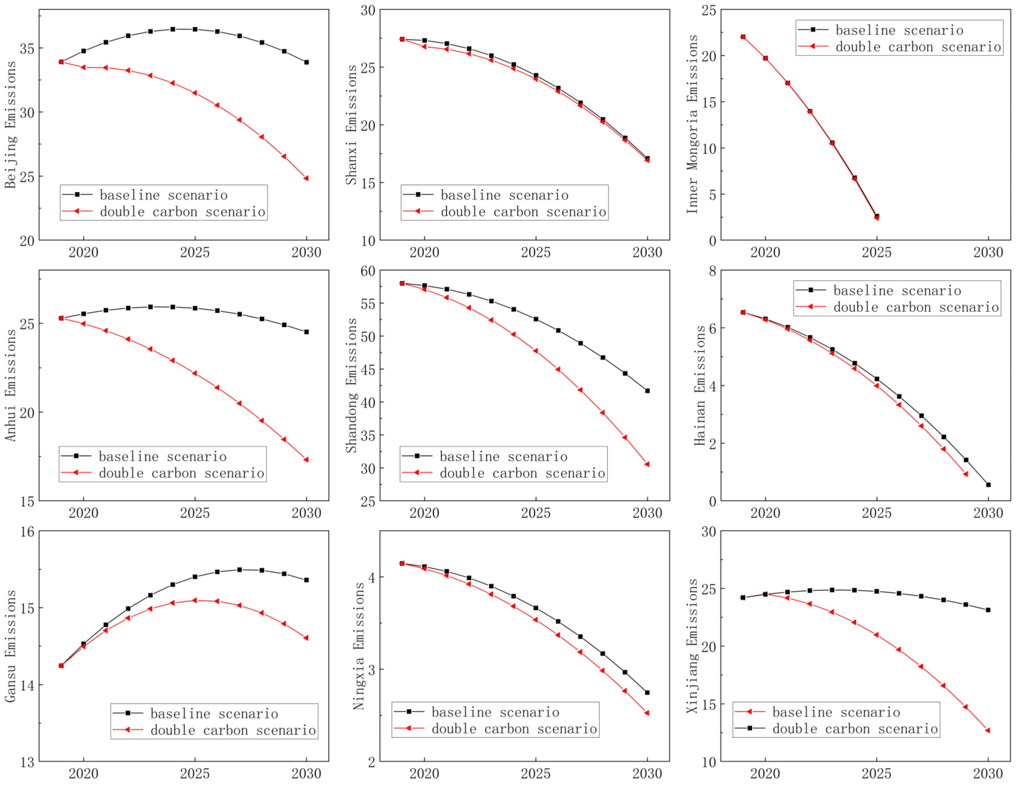
4.1. Carbon Peak Scenario Setting

The demand for TCE is positively related to the scale of economic development and technological progress, but when it reaches a certain level, the carbon emissions tend to stabilize and continue to decline [36]. The scenario prediction method is based on the energy consumption in the transportation field of China with different influencing factors in recent years to determine the baseline scenario and the carbon peaking and carbon neutralization scenario.
The high carbon scenario is unlikely to occur under the current pressure of Chinese emission reduction and national emission reduction efforts. Under each scenario, the growth rate of each energy consumption data set involved in the transportation field is set, and the future development trend of carbon emissions and intensity in China’s transportation field is predicted based on Formula (15).
The baseline scenario refers to the scenario state obtained from the historical development of decision objects and decision-driving factors, which is the benchmark set for all scenarios. The carbon peaking and carbon neutralization scenario refers to the perspective of forward push and backtracking scenarios. This study establishes the energy consumption growth rate with regional specificity, considering the spatial clustering differences in the transportation sector and China’s carbon peaking and carbon neutralization target. Through this analytical approach, short-term and long-term correlations, as well as trends, are assessed and examined.
Based on the results of TCE accounting data, the average growth rates of provinces in China from 2005 to 2010 and from 2015 to 2020 are calculated (Table 4). The calculation results show that the average growth rate of provinces and cities from 2005 to 2010 is higher than that from 2015 to 2020, showing an apparent downward trend. Beijing has the largest decline, and the growth rate of TCE has decreased from 16.3% to 4%. The average growth rate of some provinces from 2015 to 2020 is negative. In recent years, national, provincial, and municipal CER actions in transportation have achieved some results. The carbon peaking and carbon neutrality goal brings more excellent opportunities and challenges to provincial and municipal transportation planning, operation, and management. Taking into account the characteristics of the ARIMA model [37], this paper sets the source of the carbon peaking and carbon neutralization scenario as the average growth rate of each province and city in the past five years decreased by 50% compared with the benchmark scenario (In the context of the carbon peak and carbon neutrality goals, all provinces and cities in China have formulated action plans, and the impact of the COVID-19 epidemic on transportation will reduce the growth rate of carbon emissions to varying degrees. Adopt a compromise plan and take the average growth rate of all provinces and cities in the past five years as 50%). In addition, the ARIMA model is more accurate in short-term prediction. The prediction time range of this paper is 2030.

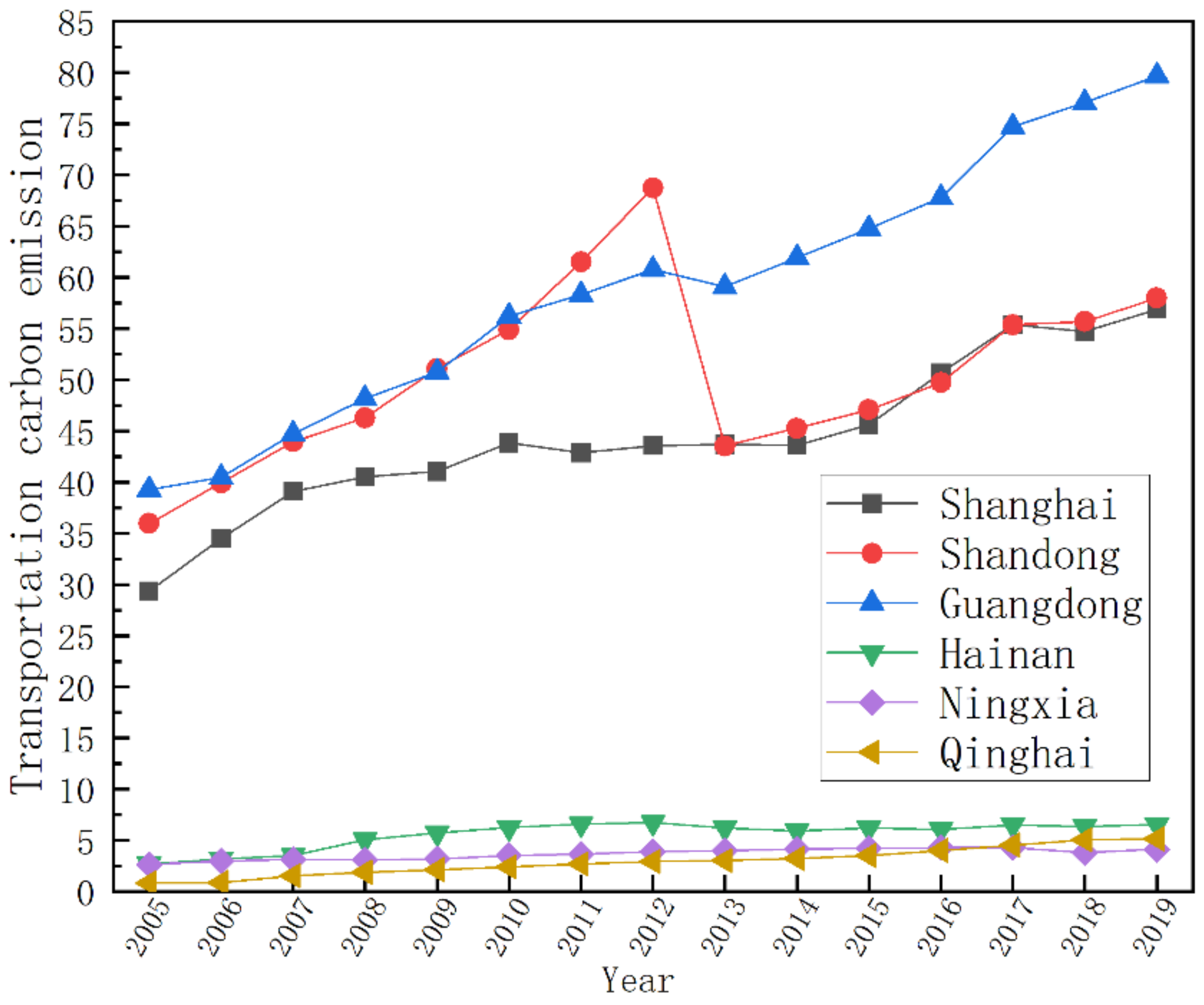
4.2. Prediction Result Analysis

The future prediction of TCE is mainly based on scenario analysis, and the ARIMA prediction method is applied. Considering that the existing research focuses on the carbon emission and emission reduction potential of the mid-long-term time nodes in 2030, 2040, and 2050, this paper sets the research node as 2030 and analyzes the changing trend of China’s provincial TCE.
The ARIMA prediction model of each province and city is constructed based on the data analysis results. It can be concluded from the forecast results that with strong policy support, the growth of carbon emissions in China’s future transportation sector can be effectively controlled, and the total carbon emissions in the “two-carbon” scenario will be reduced to different degrees compared with the baseline scenario. As is shown in Figure 2, there are 12 provinces and cities with a downward trend in the forecast of transportation carbon emissions, including Beijing, Shanxi, Inner Mongolia, Jilin, Heilongjiang, Zhejiang, Anhui, Shandong, Hainan, Gansu, Ningxia, and Xinjiang. Many regions actively adopt relevant CER policies [38]. For example, Beijing actively promotes the carbon-inclusive action of green travel; Shanxi makes great efforts to develop clean energy such as solar energy, wind energy, and hydropower to produce “green electricity” and improve the utilization rate of clean energy; Beijing and Inner Mongolia start cross-regional carbon emission trading to reduce atmospheric pollutants effectively.

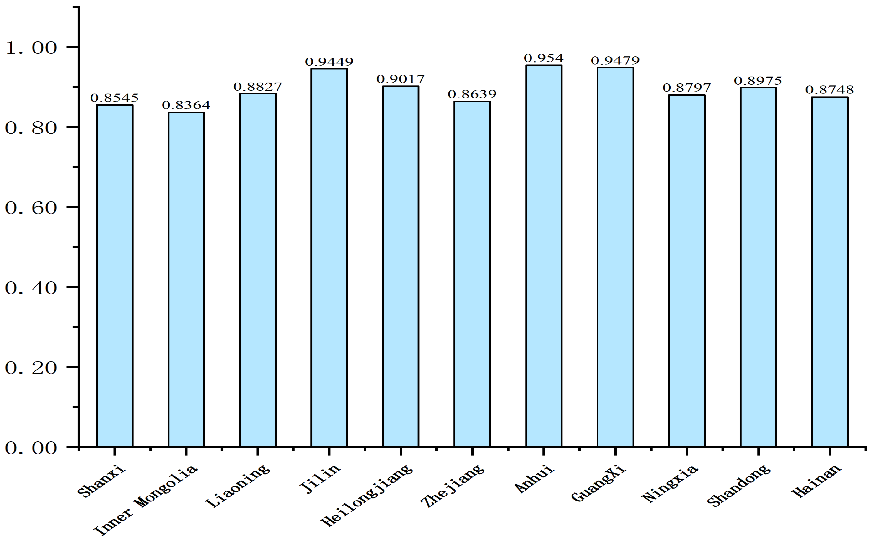
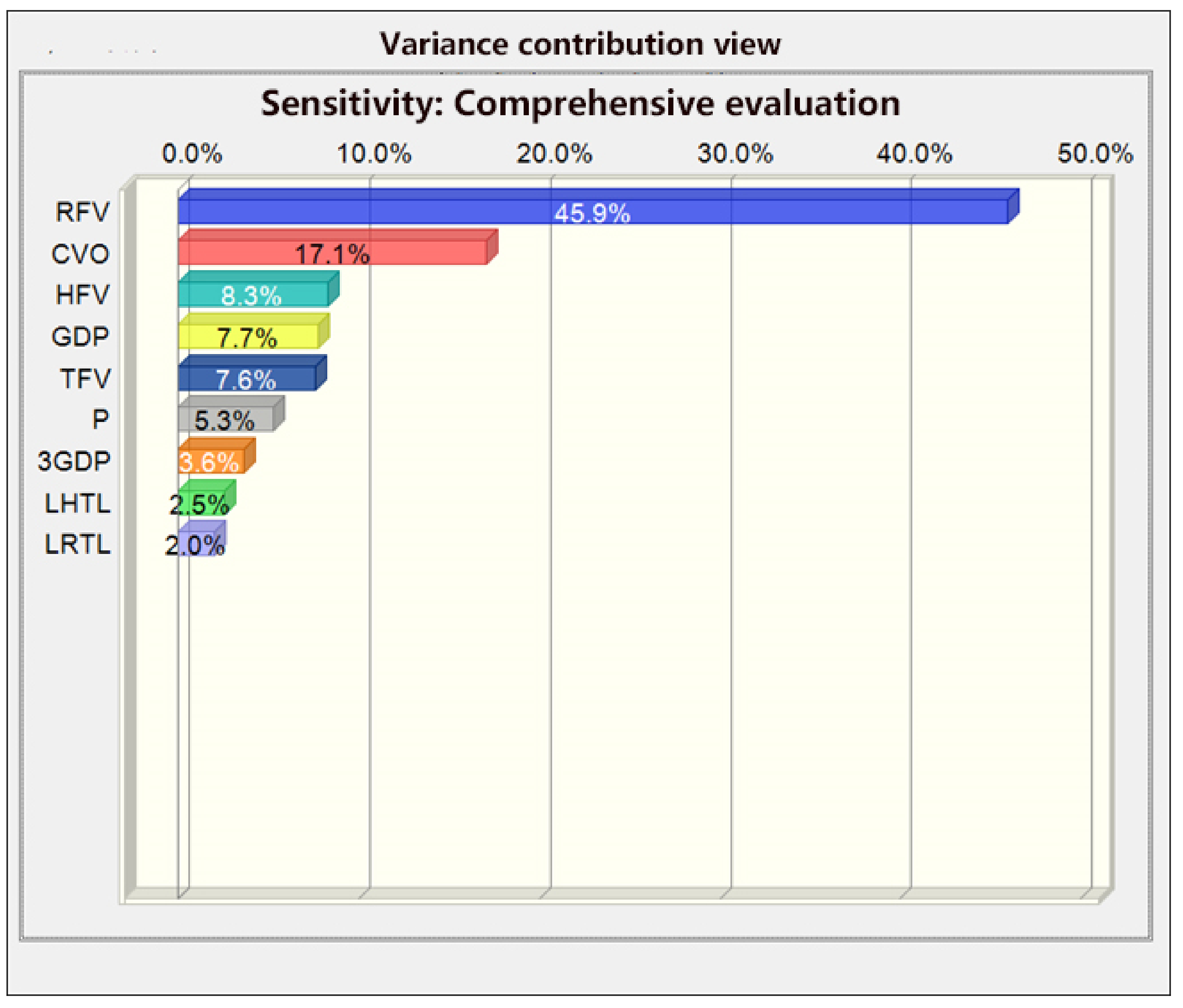
4.3. Comprehensive Evaluation

Based on the results of scenario prediction and original data, the 11 provinces and cities that have reached the peak of carbon emission in transportation are summarized as the research objects, and a comprehensive judgment system of transport carbon peaking CO2 emissions is constructed. The peak years of CO2 emissions in the 11 provinces and cities in peak CO2 emissions are shown in Table 5. For the comprehensive judgment system, the index data is the system’s input.
SPSS calculates the data in Table 6, the weight calculation result of the entropy weight method. According to the results, the weight of each index is analyzed, and it is essential to note that the weight is calculated according to the behavior unit because the index of fuzzy comprehensive evaluation refers to the line, so the weight of the line is needed.
As can be seen from Table 6, 11 indicators (Shanxi, Inner Mongolia, Liaoning, Jilin, Heilongjiang, Zhejiang, Anhui, Guangxi, Ningxia, Shandong, Hainan) and nine comments summarized according to the previous literature (GDP, GDP of the tertiary industry, population, railway transport line length, highway transport line length, total freight volume, railway freight volume, highway freight volume, and civil automobile-owned) are evaluated by fuzzy comprehensive evaluation. The weighted averaging operator M(*,+) is used. It can comprehensively use index weight and input data information, suitable for the situation with many factors, and can avoid information loss to the greatest extent.
Firstly, from the evaluation index weight vector A (which can be obtained by the entropy weight method), the weight judgment matrix R of 11 × 9 is constructed. Finally, the membership degrees of nine comment sets are obtained by analysis, which are 0.1132, 0.1295, 0.0751, 0.0526, 0.0515, 0.1044, 0.2321, 0.1083, and 0, respectively.
It can be seen from Table 7 that based on the set maximum membership rule, the general result with the highest weight in the nine comment sets is “railway freight volume”. The comprehensive evaluation index corresponding to the nine indexes in the peak year is calculated based on the previously computed index weights and other data. In Figure 3, the evaluation indexes of 10 provinces and cities are all greater than 0.85, with a probability of 90%, and the average index of each corresponding index reaches 0.8944. Among them, the average values of each index are GDP (0.0764), tertiary industry GDP (0.0892), population (0.0801), railway transportation line length (0.0843), highway transportation line length (0.0875), total freight volume (0.0736), railway freight volume (0.0840), road freight volume (0.0697), and civilian vehicle ownership (0.0871). According to the calculated index results, in addition to the corresponding indicators that reflect the scale of economic development, such as the GDP of the tertiary industry, the indicators that reflect the traffic structure, such as the length of highway transportation lines, railway freight volume and the number of civil cars, are also more significant.
We use the Monte Carlo analysis method to analyze the uncertainty of the provinces’ and cities’ fuzzy evaluation results that have reached the peak traffic carbon. By estimating the probability distribution of object variables, this method further carries out a risk assessment and sensitivity analysis of the experimental process. A Crystal ball was used to conduct a Monte Carlo analysis simulation in the test process. Generally, when the certainty of simulation results is greater than 0.85, it indicates robustness. In addition, the Monte Carlo model can find the main influencing factors from many indicators, analyze their sensitivity, and then judge the risk tolerance.
The Monte Carlo simulation results are shown in Figure 4 and Figure 5, which deal with the comprehensive judgment system’s uncertainty analysis of the transport carbon peaking CO2 emissions. Various indexes of traffic carbon emission in different provinces and cities were calculated, and 10,000 random sampling experiments were carried out. The experimental results show that the number of effective presentations is 9956 times, while the results of the probability distribution diagram show that the probability that the result index is greater than 0.85 is greater than 95%, which indicates that the results are relatively stable and feasible under the comprehensive judgment system of transportation carbon emissions, which can well explain the judgment of transport carbon peaking CO2 emissions. The sensitivity analysis chart of each index shows the sensitivity of the nine influencing factors: railway freight volume (RFV), total freight volume (CVO), road freight volume (HFV), GDP, population (P), tertiary industry GDP (3GDP), road transport line length (LHTL) and railway transport line length (LRTL) in descending order. Among them, the indicators representing the freight volume of railways and highways and the total freight volume are particularly significant, while other indicators have high uncertainty.

5. Conclusions, Actions, and Recommendations

5.1. Conclusions

Through the comprehensive autoregressive moving average model, an ARIMA prediction model considering data endogeneity is built for 30 provinces and cities, and two dynamic scenarios are set up, namely, the baseline scenario and the carbon peak and carbon neutralization scenario, to simulate the peak path of Chinese future carbon emissions and the changing trend of carbon emissions in each province and city.
Research findings: Firstly, the TCE sector’s expansion in the future can be effectively managed with robust policy backing [39]. The total carbon emissions in the carbon peak and carbon neutralization scenario are decreased to different extents when compared to the baseline scenario. Secondly, the comprehensive evaluation index for the peak year is higher than 0.85, and the output score continues to be higher than 0.85 even after the peak year. Provided that a province fulfills the aforementioned fundamental prerequisites, except for any potential exceptional circumstances, it is initially ascertained that the region possesses a 95% likelihood of having attained the pinnacle of transportation carbon dioxide emissions. Thirdly, the sensitivity of nine indicators in the comprehensive research and judgment system for carbon peak in transportation is as follows: large to small: railway freight volume, total freight volume, road freight volume, GDP, population, tertiary industry GDP, road transport line length, and railway transport line length.

5.2. Actions and Recommendations

According to ITF Transport Outlook 2021, through policy guidance, TCE can be reduced by nearly 70% from 2015 to 2050. Achieving the carbon peaking and carbon neutrality goal will require implementing a series of emission reduction measures. Specific directions mainly include formulating a regionally differentiated emission reduction development strategy; developing public transport and active transport; increasing financial investment, especially science and technology expenditure [40]; improving energy utilization efficiency in the transportation field through technological progress; building a transportation network structure with the characteristics of each province, city, and region under the background of the development of the Internet of Vehicles and the Internet of Things technology [41]; and reducing the consumption of “connotation energy”.
It is essential to explore the action plan for transportation carbon reduction and emission reduction strategies in line with the different development backgrounds of various provinces and cities in China and carry out relevant research [42]. Based on the analysis of pertinent results of this paper, for cities that have reached the peak or are standing in the platform period, action plans for total CER should be established; for cities that have not yet reached the peak, the goal of reaching the peak and peak year should be clearly defined, the promotion plan for carbon emission peak action should be established, and the peak should be reached as early as possible; for cities in the transition period of traditional industries, low carbon potential cities, and resource-based cities, it is necessary to distinguish the situation and make the best use of each individual case to establish an action plan toward its carbon peak as soon as possible, to reduce carbon emissions and enter the carbon peak stage as soon as possible.

5.3. Study Limitations

This paper’s carbon-peaking comprehensive research and judgment system has a certain level of stability. If the economy and society are subject to unforeseen or uncontrollable circumstances that result in drastic shifts beyond the scope of expected possibility, the system may struggle to carry out judgment. Despite taking into account the historical development situation and future planning, in order to reach the state transportation carbon peak in China’s provinces and cities in the future, certain uncertainties need to be addressed.

Author Contributions

Conceptualization, Y.S., Y.Y., S.L. and Q.L.; formal analysis, Y.S., Y.Y. and S.L.; funding acquisition, Y.S.; methodology, Y.S., Y.Y., S.L. and Q.L.; writing—original draft, Y.Y.; writing—review and editing, Y.S. and Q.L. All authors have read and agreed to the published version of the manuscript.

Funding

This research was funded by the Shandong Natural Science Foundation (Grant number ZR2021MG021).

Institutional Review Board Statement

Not applicable.

Informed Consent Statement

Not applicable.

Data Availability Statement

Data sharing is not applicable. No new data were created or analyzed in this study.

Conflicts of Interest

The authors declare no conflict of interest.

References

  1. Sun, Y.; Liu, S.; Li, L. Grey Correlation Analysis of Transportation Carbon Emissions under the Background of Carbon Peak and Carbon Neutrality. Energies 2022, 15, 3064. [Google Scholar] [CrossRef]
  2. Yu, Y.; Li, S.; Sun, H.; Taghizadeh-Hesary, F. Energy carbon emission reduction of China’s transportation sector: An input–output approach. Econ. Anal. Policy 2021, 69, 378–393. [Google Scholar] [CrossRef]
  3. Wang, Y.; Zhou, Y.; Zhu, L.; Zhang, F.; Zhang, Y. Influencing factors and decoupling elasticity of China’s transportation carbon emissions. Energies 2018, 11, 1157. [Google Scholar] [CrossRef]
  4. Li, Y.; Zhang, Q. Research on carbon emission reduction based on the optimization of transportation structure under VAR model. IOP Conf. Ser. Earth Environ. Sci. 2020, 440, 042008. [Google Scholar] [CrossRef]
  5. Liu, Y.; Chen, L.; Huang, C. Study on the carbon emission spillover effects of transportation under technological advancements. Sustainability 2022, 14, 10608. [Google Scholar] [CrossRef]
  6. Prasad, R.D.; Raturi, A. Low-carbon measures for Fiji’s land transport energy system. Util. Policy 2018, 54, 132–147. [Google Scholar] [CrossRef]
  7. Selvakkumaran, S.; Limmeechokchai, B. Low carbon society scenario analysis of transport sector of an emerging economy—The AIM/Enduse modelling approach. Energy Policy 2015, 81, 199–214. [Google Scholar] [CrossRef]
  8. Gao, J.; Pan, L. A System Dynamic Analysis of Urban Development Paths under Carbon Peaking and Carbon Neutrality Targets: A Case Study of Shanghai. Sustainability 2022, 14, 15045. [Google Scholar] [CrossRef]
  9. Zhang, C.; Luo, H. Research on carbon emission peak prediction and path of China’s public buildings: Scenario analysis based on LEAP model. Energy Build. 2023, 289, 113053. [Google Scholar] [CrossRef]
  10. Gonçalves, D.N.S.; Goes, G.V.; D’Agosto, M.d.A.; La Rovere, E.L. Development of Policy-Relevant Dialogues on Barriers and Enablers for the Transition to Low-Carbon Mobility in Brazil. Sustainability 2022, 14, 16405. [Google Scholar] [CrossRef]
  11. Liimatainen, H.; Kallionpää, E.; Pöllänen, M.; Stenholm, P.; Tapio, P.; McKinnon, A. Decarbonizing road freight in the future—Detailed scenarios of the carbon emissions of Finnish road freight transport in 2030 using a Delphi method approach. Technol. Forecast. Soc. 2014, 81, 177–191. [Google Scholar] [CrossRef]
  12. Dhar, S.; Pathak, M.; Shukla, P.R. Transformation of India’s transport sector under global warming of 2 °C and 1.5 °C scenario. J. Clean Prod. 2018, 172, 417–427. [Google Scholar] [CrossRef]
  13. Wang, X.; Zhou, Y.; Bi, Q.; Cao, Z.; Wang, B. Research on the Low-Carbon Development Path and Policy Options of China’s Transportation Under the Background of Dual Carbon Goals. Front. Environ. Sci. 2022, 10, 905037. [Google Scholar] [CrossRef]
  14. AlSabbagh, M.; Siu, Y.L.; Guehnemann, A.; Barrett, J. Integrated approach to the assessment of CO2 emitigation measures for the road passenger transport sector in Bahrain. Renew. Sust. Energy Rev. 2017, 71, 203–215. [Google Scholar] [CrossRef]
  15. Wang, C.; Cai, W.; Lu, X.; Chen, J. CO2 mitigation scenarios in China’s road transport sector. Energy Convers. Manag. 2007, 48, 2110–2118. [Google Scholar] [CrossRef]
  16. Gao, B.; Sun, X. Analysis on temporal change and grey relation of transportation carbon emissions in Jilin Province. IOP Conf. Ser. Earth Environ. Sci. 2018, 146, 012009. [Google Scholar] [CrossRef]
  17. Wu, Y.; Zhou, Y.; Liu, Y.; Liu, J. A Race Between Economic Growth and Carbon Emissions: How Will the CO2 Emission Reach the Peak in Transportation Industry? Front. Energy Res. 2022, 9, 778757. [Google Scholar] [CrossRef]
  18. Byers, E.A.; Gasparatos, A.; Serrenho, A.C. A framework for the exergy analysis of future transport pathways: Application for the United Kingdom transport system 2010–2050. Energy 2015, 88, 849–862. [Google Scholar] [CrossRef]
  19. Tang, B.-J.; Li, X.-Y.; Yu, B.; Wei, Y.-M. Sustainable development pathway for intercity passenger transport: A case study of China. Appl. Energy 2019, 254, 113632. [Google Scholar] [CrossRef]
  20. Fernández-Dacosta, C.; Shen, L.; Schakel, W.; Ramirez, A.; Kramer, G.J. Potential and challenges of low-carbon energy options: Comparative assessment of alternative fuels for the transport sector. Appl. Energy 2019, 236, 590–606. [Google Scholar] [CrossRef]
  21. Zhou, G.; Chung, W.; Zhang, X. A study of carbon dioxide emissions performance of China’s transport sector. Energy 2013, 50, 302–314. [Google Scholar] [CrossRef]
  22. Talbi, B. CO2 emissions reduction in road transport sector in Tunisia. Renew. Sust. Energy Rev. 2017, 69, 232–238. [Google Scholar] [CrossRef]
  23. Mattioli, G. Transport needs in a climate-constrained world. A novel framework to reconcile social and environmental sustainability in transport. Energy Res. Soc. Sci. 2016, 18, 118–128. [Google Scholar] [CrossRef]
  24. Fan, F.; Lei, Y. Decomposition analysis of energy-related carbon emissions from the transportation sector in Beijing. Transp. Res. Part D Transp. Environ. 2016, 42, 135–145. [Google Scholar] [CrossRef]
  25. Xu, B.; Lin, B. Differences in regional emissions in China’s transport sector: Determinants and reduction strategies. Energy 2016, 95, 459–470. [Google Scholar] [CrossRef]
  26. Tsita, K.G.; Pilavachi, P.A. Decarbonizing the Greek road transport sector using alternative technologies and fuels. Therm. Sci. Eng. Prog. 2017, 1, 15–24. [Google Scholar] [CrossRef]
  27. Zhang, Q.; Gu, B.; Zhang, H.; Ji, Q. Emission reduction mode of China’s provincial transportation sector: Based on “Energy+” carbon efficiency evaluation. Energy Policy 2023, 177, 113556. [Google Scholar] [CrossRef]
  28. Chen, Q.; Wang, Q.; Zhou, D.; Wang, H. Drivers and evolution of low-carbon development in China’s transportation industry: An integrated analytical approach. Energy 2023, 262, 125614. [Google Scholar] [CrossRef]
  29. Wang, M.; Zhu, C.; Cheng, Y.; Du, W.; Dong, S. The influencing factors of carbon emissions in the railway transportation industry based on extended LMDI decomposition method: Evidence from the BRIC countries. Environ. Sci. Pollut. Res. 2023, 30, 15490–15504. [Google Scholar] [CrossRef] [PubMed]
  30. Kour, M. Modelling and forecasting of carbon-dioxide emissions in South Africa by using ARIMA model. Int. J. Environ. Sci. Technol. 2023, 20, 11267–11274. [Google Scholar] [CrossRef]
  31. Du, Y.-W.; Wang, S.-S.; Wang, Y.-M. Group fuzzy comprehensive evaluation method under ignorance. Expert Syst. Appl. 2019, 126, 92–111. [Google Scholar] [CrossRef]
  32. Eggleston, H.S.; Buendia, L.; Miwa, K.; Ngara, T.; Tanabe, K. 2006 IPCC Guidelines for National Greenhouse Gas Inventories; Chapter 6; Institute for Global Environmental Strategies: Kanagawa, Japan, 2006; Volume 2, pp. 5–7. ISBN 4-88788-032-4. [Google Scholar]
  33. GB/T2589-2020; General Principles for Calculation of Comprehensive Energy Consumption. Standardization Administration of China: Beijing, China, 2020. (In Chinese)
  34. Eggleston, H.S.; Buendia, L.; Miwa, K.; Ngara, T.; Tanabe, K. 2006 IPCC Guidelines for National Greenhouse Gas Inventories; Chapter 2; Institute for Global Environmental Strategies: Kanagawa, Japan, 2006; Volume 2, pp. 16–23. ISBN 4-88788-032-4. [Google Scholar]
  35. DB11/T 1785-2020; Requirements for Carbon Dioxide Emission Accounting and Reporting Power Generation Enterprises. China Beijing Local Standard Press: Beijing, China, 2020. (In Chinese)
  36. Ye, L.; Yang, D.; Dang, Y.; Wang, J. An Enhanced Multivariable Dynamic Time-Delay Discrete Grey Forecasting Model for Predicting China’s Carbon Emissions. Energy 2022, 249, 123681. [Google Scholar] [CrossRef]
  37. Garg, N.; Soni, K.; Saxena, T.K.; Maji, S. Applications of AutoRegressive Integrated Moving Average (ARIMA) approach in time-series prediction of traffic noise pollution. Noise Control. Eng. J. 2015, 63, 182–194. [Google Scholar] [CrossRef]
  38. Zhan, D. Allocation of carbon emission quotas among provinces in China: Efficiency, fairness and balanced allocation. Environ. Sci. Pollut. Res. 2022, 29, 21692–21704. [Google Scholar] [CrossRef] [PubMed]
  39. Zhu, C.; Wang, M.; Yang, Y. Analysis of the Influencing Factors of Regional Carbon Emissions in the Chinese Transportation Industry. Energies 2020, 13, 1100. [Google Scholar] [CrossRef]
  40. Zhuang, X.; Li, X.; Xu, Y. How Can Resource-Exhausted Cities Get Out of “The Valley of Death”? An Evaluation Index System and Obstacle Degree Analysis of Green Sustainable Development. Int. J. Environ. Res. Public Health 2022, 19, 16976. [Google Scholar] [CrossRef] [PubMed]
  41. Zhao, B.; Sun, L.; Qin, L. Optimization of China’s provincial carbon emission transfer structure under the dual constraints of economic development and emission reduction goals. Environ. Sci. Pollut. R 2022, 29, 50335–50351. [Google Scholar] [CrossRef]
  42. Sun, H.; Hu, L.; Geng, Y.; Yang, G. Uncovering impact factors of carbon emissions from transportation sector: Evidence from China’s Yangtze River Delta Area. Mitig. Adapt. Strateg. Glob. Change 2020, 25, 1–15. [Google Scholar] [CrossRef]
Figure 1. Statistics of TCE in some provinces from 2005 to 2019.
Sustainability 15 14880 g001
Figure 2. Statistical Chart of Carbon TCE Forecast in a Downward Trend.
Sustainability 15 14880 g002
Figure 3. Comprehensive evaluation index corresponding to 9 indicators in the peak year.
Sustainability 15 14880 g003
Figure 4. System uncertainty analysis diagram.
Sustainability 15 14880 g004
Figure 5. System sensitivity analysis diagram.
Sustainability 15 14880 g005
Table 1. Variable name and corresponding formula.
Variable NameCorresponding FormulaS/N
Mean value μ = E ( X t ) (1)
Variance σ 2 = D X t = E X t μ 2 (2)
Standard deviation σ = D ( X t ) 2 (3)
Autocovariance (Unbiased) c k = 1 N k t = k 1 N x t μ ( x t k μ ) (4)
Autocovariance (Biased) c ^ k = E X t μ X t k μ = 1 N t = k 1 N x t μ ( x t k μ ) (5)
Table 2. Statistical description of energy carbon emission factors.
EnergyAverage Low Calorific ValueCarbon Content per Unit Calorific ValueCarbon Oxidation RateCarbon Emission Factor
UnitkJ/kg or kJ/m3t-c or TJ kg-CO2 or kg
raw coal20,93427.370.941.975
gasoline43,12418.90.982.929
kerosene43,12419.50.983.022
diesel42,70520.20.983.010
fuel oil41,86821.10.983.174
liquefied petroleum gas50,24217.20.983.105
natural gas32,23815.320.991.793
Table 3. China’s regional electricity carbon emission coefficient.
RegionCovering Provinces, Districts, and CitiesCO2 Emission Coefficient
(kg/KW·h)
North ChinaBeijing, Tianjin, Hebei, Shaanxi, Shandong, Western Inner Mongolia1.246
Northeast RegionLiaoning, Jilin, Heilongjiang, Eastern Inner Mongolia1.096
East ChinaShanghai, Jiangsu, Zhejiang, Anhui, Fujian0.928
Central ChinaHenan, Hubei, Hunan, Jiangxi, Sichuan0.801
Northwest RegionShaanxi, Gansu, Qinghai, Ningxia, Xinjiang0.977
Southern regionGuangdong, Guangxi, Yunnan, Guizhou0.714
Other areasHainan0.917
Note: Considering the data statistics, the eastern and western regions of Inner Mongolia are uniformly calculated according to North China’s CO2 emission coefficient.
Table 4. Average growth rate of TCE in China’s provinces.
Provinces2005–2010 Growth Rate2015–2020 Growth RateCarbon Peaking and Carbon Neutralization Growth RateProvinces2005–2010 Growth Rate2015–2020 Growth RateCarbon Peaking And Carbon Neutralization Growth Rate
Beijing0.1633930.0399290.019964Henan0.0895420.0865040.043252
Tianjin0.0778170.0324530.016226Hubei0.0625330.0719070.035953
Hebei0.0644590.0481320.024066Hunan0.0852290.0484960.024248
Shanxi0.1322550.0208960.010448Guangdong0.07430.04230.02115
IM0.156804−0.0450.090007Guangxi0.1036710.0315710.015785
Liaoning0.0578780.0112970.005648Hainan0.1846060.0105890.005294
Jilin0.115844−0.02529−0.05058Chongqing0.1096480.0953150.047658
Heilongjiang0.026716−0.02624−0.05247Sichuan0.1126680.0970860.048543
Shanghai0.0833760.0451460.022573Guizhou0.1570190.0287920.014396
Jiangsu0.0976210.0454830.022742Yunnan0.0922790.0602890.030144
Zhejiang0.0947410.007940.00397Shaanxi0.1459020.0188940.009447
Anhui0.123260.0281590.014079Gansu0.0780810.0111270.005564
Fujian0.1426390.0596670.029834Qinghai0.2327110.0782240.039112
Jiangxi0.075330.0539020.026951Ningxia0.059488−0.00463−0.00927
Shandong0.0883110.0425590.02128Xinjiang0.0447880.029550.014775
Total0.0946990.0384160.01920
Note: IM stands for Inner Mongolia.
Table 5. Annual statistics of CO2 peak in provinces and cities with traffic carbon peak.
Peak ProvinceShanxiInner MongoliaLiaoningJilinHeilongjiangZhejiangAnhuiGuangxiNingxiaShandongHainan
Peak time20172012201720152016201720182018201720192019
Table 6. Initial weight statistics.
Entropy Method
TermShannon Entropy (e)Information Utility (d)Weight (%)
Shanxi0.7010.2997.989
Inner Mongolia0.6970.3038.113
Liaoning0.6570.3439.186
Jilin0.6750.3258.701
Heilongjiang0.6350.3659.778
Zhejiang0.6630.3379.03
Anhui0.5960.40410.823
Guangxi0.6410.3599.61
Ningxia0.6710.3298.813
Shandong0.6950.3058.154
Hainan0.6340.3669.802
Table 7. Calculation results of the membership matrix.
Index ItemMembership DegreeNormalization of Membership Degree (Weight)
GDP0.0584643450.113249657
GDP of the tertiary industry0.0288973780.129508773
Population0.0098903180.075106036
Railway transport line length0.0113647050.052662112
Highway transport line Length0.3333126780.051549757
Total freight volume0.4277627860.104439486
Railway freight volume0.0460648720.232147967
Highway freight volume0.3148563550.108263984
Civil automobile-owned0.0013687230.13307223
Disclaimer/Publisher’s Note: The statements, opinions and data contained in all publications are solely those of the individual author(s) and contributor(s) and not of MDPI and/or the editor(s). MDPI and/or the editor(s) disclaim responsibility for any injury to people or property resulting from any ideas, methods, instructions or products referred to in the content.

