Impacts of Land Use Intensity on Ecosystem Services: A Case Study in Harbin City, China

Abstract

Land use intensity (LUI) is an important indicator for assessing human activities, and quantitatively studying the impact of LUI on ESs can help to realize the scientific management of urban ecosystems as well as sustainable development. In this study, we quantified five important ecosystem service bundles in the study area with the aid of the R-language “kohonen” package and used bivariate spatial autocorrelation modeling to examine the effects of LUI on the ESs in Harbin City from 2000 to 2020. These ESs include food supply (FP), water conservation (WC), soil conservation (SC), carbon storage (CS), water purification (WP), and habitat quality (HQ). The results show the following: (1) The LUI in Harbin City had a trend from 2000 to 2020 of “decreasing and then growing”, with a spatial distribution pattern of “high in the west and low in the east.” (2) Except for FP, all other ESs exhibit a similar spatial pattern of “west-low-east-high”; WC and WP exhibit a trend of continuous increase, SC exhibits a trend of decreasing and then increasing, and CS and HQ are generally more stable, with less fluctuation. The built-up area is situated in the high-value area of LUI, and the area exhibits a significant expansion trend. (3) Ecological conservation bundles, FP–WP synergistic bundles, ecological transition bundles, CS–WP–HQ synergistic bundles, and FP bundles are the five ecosystem service bundles that were discovered in Harbin. (4) From 2000 to 2020, there is a predominately “low LUI-high ESs” and “high LUI-low ESs” aggregation type, with a substantial positive correlation between LUI and FP and a significant negative correlation between LUI and other ESs. Harbin City should strengthen the management of ESs in the western part of the city and, at the same time, maintain the favorable ecological conditions in the ecological barriers of Zhangguangcai Range and Xiaoxing’an Mountains.

1. Introduction

Ecosystem services (ESs) are the benefits that people gain from ecosystems [1], either directly or indirectly. They are viewed as a crucial link between natural ecosystems and socio-economic systems [2,3], which is crucial for improving human well-being. For example, water conservation services reflect the ability of ecosystems to intercept precipitation and regulate runoff [4]. Soil conservation helps to regulate the erosive effects of soil loss [5]. Water purification services characterize the degree of purification and retention of pollutants [6]. ESs are essential for preserving ecosystem stability and fostering the growth of a healthy natural environment [7,8]. Humans are putting more and more emphasis on the research of ESs’ distribution patterns and underlying mechanisms as a result of their significant utility [9,10,11]. The conflicts between human activities and natural ecosystems have become increasingly evident as urbanization has progressed [12,13,14]. Numerous studies have confirmed that changes in land use structure and state will result in the fragmentation of natural habitats, which will then change the structure and function of ecosystems and hurt biodiversity and ESs [15]. Therefore, it is crucial to thoroughly research how human actions affect ESs.

Land use change will cause changes in the structure, function, and efficiency of land use [16], and land use intensity (LUI) is a key indicator of human activities, which to a certain extent can reflect the degree of human activities’ interference [17,18]. The more frequently human activities occur in the area, the higher the land use intensity. Large-scale exploitation of land use by human activities is prone to lead to significant changes in the ecological environment, or even rapid degradation, thus directly affecting the role played by ESs. Modifying soil characteristics, biochemical cycles, and biodiversity through a variety of ecological processes can also have an indirect impact on the quality of ESs [19]. Different ESs may be positively or negatively correlated with LUI, and exploring the influence of LUI on ESs can reflect the degree of threat to ecosystems from human activities. Currently, scholars at home and abroad have achieved rich results in this area, but the research content is mostly focused on the impact of land use change on the ecological environment and the contribution of land use change to ESs [20,21]. The quantitative methods are mostly land use transfer matrix [22], land use dynamics [23,24], and correlation analysis [25], and there are fewer quantitative and in-depth analyses of the spatial relationship between LUI and ESs, which limits the guidance significance of LUI regulation for the optimization of ESs to some degree.

The Integrated Valuation of Ecosystem Services and Trade-offs (InVEST) model has been widely used in assessment studies of ESs because of its simplicity of operation and easy access to data [26,27]. Currently, it has been applied in regions such as Kentucky, Ethiopia, and the Transalpine region [28,29,30,31], and it is combined with the PLUS model, geodetector, and geographically weighted regression to delve deeper into the drivers or future scenario simulations of ESs [32,33,34]. Therefore, in this study, the InVEST model was selected to assess the ESs and it was combined with the bivariate spatial autocorrelation model to further explore the relationship between the response of ESs to LUI.

The natural ecosystem of Harbin, a typical industrial city in China, has been severely impacted, and the ecological environment there is still unsustainable due to the growth of urbanization and the unique climatic influences of the cold zone [35]. There is a relatively unequal distribution of water resources in the area, and permafrost degradation has become worse recently, lowering the stability of local water resources and interfering with ecological processes [36,37]. The water quality of rivers and lakes has been declining as a result of the extensive cultivation of food crops and the use of chemical fertilizers and pesticides in enormous quantities [38]. According to the comprehensive water quality index, Harbin has reached the level of heavy pollution.

In conclusion, this paper chooses six key indicators to quantify ESs in Harbin City: food supply (FP), water conservation (WC), soil conservation (SC), carbon storage (CS), water purification (WP), and habitat quality (HQ). It also investigates the spatial and temporal characteristics of the ESs in the study area from 2000 to 2020 based on the InVEST model to identify the key five bundles of ESs and introduces a bivariate spatial autocorrelation model to deeply explore the impacts of the LUI on the ESs. The main contributions of this study include (1) assessing the spatial and temporal evolution of LUI and ESs in Harbin City from 2000 to 2020 and exploring the relationship between the response of ESs to LUI; (2) based on the identification of hotspot areas and the impact of LUI on ESs, dividing the land space of Harbin City into three major functional subdivisions, namely, ecological governance, ecological enhancement, and ecological protection; and (3) based on the characteristics of different ecological functional subdivisions, providing scientific recommendations on the management of land space in Harbin City. For example, the western part of the city is dominated by governance and focuses on the maintenance of FP, while the northern and eastern parts of the city are dominated by protection and large-scale human interference is strictly prohibited.

2. Materials and Methods

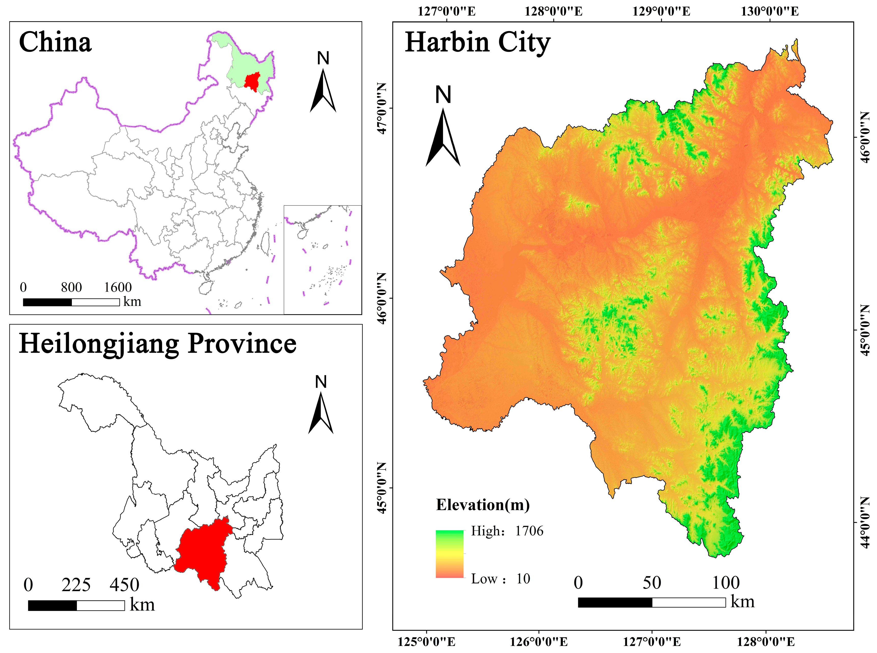
2.1. Overview of the Study Area

As a typical industrial city in northern China, Harbin has a total area of about 53,000 km² (Figure 1). Harbin is a typical industrial city with a long history, high population density [39], dense transportation, huge industrial coal consumption, and complex industrial structure [40]. Harbin City belongs to the mid-temperate continental monsoon climate, with four distinct seasons, and rainfall is mainly concentrated in summer [41]. The landform of Harbin City is high in the south and low in the north, which is an important grain production base in China.

2.2. Data Sources

The main data sources used in this study are shown in

Table 1. Data sources [42,43].

Data	Type	Data Source	Spatial Resolution	Accessed Date
Land use/land cover	Raster	GlobeLand30 (https://www.webmap.cn/commres.do?method=globeIndex)	30 m × 30 m	15 October 2022
Annual average precipitation	Raster	National Earth System Science Data Center, National Science and Technology Infrastructure of China (http://www.geodata.cn)	1 km × 1 km	15 October 2022
Reference evapotranspiration	Raster	National Earth System Science Data Center, National Science and Technology Infrastructure of China (http://www.geodata.cn)	1 km × 1 km	15 October 2022
Digital Elevation Model (DEM)	Raster	Geospatial data cloud (http://www.gscloud.cn)	30 m × 30 m	6 December 2022
NPP	Raster	U.S. Geological Survey (USGS) (https://lpdaac.usgs.gov/product_search/?view=list)	500 m × 500 m	8 March 2023
Grain production	.txt file	Harbin Statistical Yearbook (https://www.harbin.gov.cn/haerbin/c104482/list_navlist.shtml)	—	8 March 2023
Soil data	Raster	The dataset is provided by National Cryosphere Desert Data Center (http://www.ncdc.ac.cn)	1 km × 1 km	15 October 2022

.

2.3. Land Use Intensity Assessment

LUI reflects, to some extent, the intensity of anthropogenic disturbances. The formula for calculating the land use intensity index is [44]:

$$LUI=100\times \sum _{i=1}^n{A}_i\times C_i$$

(1)

where LUI means the comprehensive index of land use degree; A_i indicates the index of the land use degree classification of level i; and C_i is the percentage of the area of the land use degree classification of level i. A grid of 3 km × 3 km was used to sample the land use classification map of the study area, and 6221 sampling grids were obtained.

2.4. ESs Assessment

2.4.1. Food Supply

Harbin is one of the important grain production bases in China, with agricultural land accounting for about 50 percent of the city’s area. In this study, food supply services are quantified using NPP data and statistics yearbooks. The following calculation formula is used:

$$F_x=\frac{{NPP}_x}{NPP}\times F$$

(2)

where F_x represents the crop yield on the agricultural land grid cell x; F means the total annual crop yield in Harbin City; NPP_x is the NPP value of grid cell x in agricultural land; and NPP indicates the total annual NPP of agricultural land in Harbin city.

2.4.2. Water Conservation

The water conservation capacity refers to the amount of water that the soil layer can regulate after precipitation, minus both evapotranspiration and surface runoff. In this study, the water retention capacity was calculated by subtracting the surface runoff from the total water yield. The specific formula is as follows:

$${WR}_{xj}=Y_{xj}-{Runoff}_{xj}$$

(3)

$${Runoff}_{xj}=P_x\times C_j$$

(4)

where WR_xj represents the annual water retention of land cover type j in grid x; Y_xj denotes the annual water production of land cover type j in grid x; Runoff_xj stands for the annual surface runoff of land cover type j in grid x; P_x is the amount of precipitation in grid x; and C_j indicates the surface runoff coefficient for land cover type j.

The water yield module of the InVEST model calculates the rainfall minus evapotranspiration for each grid, mainly based on the water balance principle. The formula for water yield is:

$$Y_{xj}=\left(1-\frac{{AET}_{xj}}{P_x}\right)\times P_x$$

(5)

where Y_xj represents the water yield of land cover type j in grid x; AET_xj stands for the actual evapotranspiration of land cover type j in grid x; P_x indicates the precipitation of grid x; and AET_xj/P_x denotes the ratio of the actual evapotranspiration to the precipitation.

$$\frac{{AET}_{xj}}{P_x}=\frac{1+w_x{R}_{xj}}{1+w_x{R}_{xj}+\frac{1}{R_{xj}}}$$

(6)

$$w_x=Z\frac{{PAWC}_x}{P_x}$$

(7)

$$R_{xj}=\frac{k_{ij}\times {ET}_0}{P_x}$$

(8)

where R_xj is the Budyko dryness index of raster cell x on land cover type j; ω_x is the ratio of annual available water for vegetation to expected precipitation; Z is the Zhang coefficient; k_ij is the plant evapotranspiration coefficient, which represents the ratio of crop evapotranspiration to the reference evapotranspiration (ET₀) during the different developmental periods, with reference to the research results of the previous researchers and the user’s manual of the InVEST model [28,45], and combined with the actual assignment of the study area; and PAWC_x stands for the plant-available water content, and the specific calculation formula is as follows [46]:

$$\begin{array}{c}PAWC=54.509-0.132sand-0.003{sand}^2-0.055silt-0.006{silt}^2-\\ 0.738clay+0.007{clay}^2-2.688OM+0.501{OM}^2\end{array}$$

(9)

where sand is soil sand content; silt is soil silt content; clay is soil clay content; and OM is soil organic matter content.

2.4.3. Soil Conservation

The difference between potential soil erosion and actual soil erosion is calculated based on the USLE calculation method at the image element scale, and the result is the SC [47]. The formula is:

$${SC}_i={RKLS}_i-{USLE}_i$$

(10)

$${RKLS}_i=R_i\times K_i\times {LS}_i$$

(11)

$${USLE}_i=R_i\times K_i\times {LS}_i\times C_i\times P_i$$

(12)

where SC_i represents the annual soil conservation; RKLS_i indicates the potential soil erosion; USLE_i stands for the actual soil erosion; R is the rainfall erosivity factor; K is the soil erodibility factor; L stands for the slope length factor; S indicates the steepness factor; C represents the vegetation cover and crop management factor; and P is the soil and water conservation measures factor.

The rainfall erosivity factor (R) reflects the ability of rainfall to erode soil and was calculated in this study using the following equation:

$$R_j=\alpha P_j^{\beta }$$

(13)

where R_j is the rainfall erosive force in year j, P_j is the rainfall in year j, and α and β are model parameters.

The soil erodibility factor (K) was calculated as follows:

$$K=\left(-0.01383+0.51575K_{EPIC}\right)\times 0.1317$$

(14)

$$\begin{gathered} K_{EPIC}=\left\{0.2+0.3\exp \left[-0.0256m_s\left(1-\frac{m_{silt}}{100}\right)\right]\right\} \\ \times {\left[\frac{m_{silt}}{m_c+m_{silt}}\right]}^{0.3}\times \left\{1-\frac{0.25orgC}{\left[orgC+\exp \left(3.72-2.95orgC\right)\right]}\right\} \\ \times \left\{1-\frac{0.7\left(1-m_s/100\right)}{\left\{\left(1-m_s/100\right)+\exp \left[-5.51+22.9\left(1-m_s/100\right)\right]\right\}}\right\} \end{gathered}$$

(15)

where K is the soil erodibility factor, m_s is the sand content, m_silt is the powder content, m_c is the clay content, and orgC is the organic carbon content.

The vegetation cover and crop management factor (C) and the soil and water conservation measures factor (P) were corrected by combining the InVEST model user guide and the experience of previous researchers [48,49,50].

2.4.4. Carbon Stocks

The carbon storage module of the InVEST model is mainly based on aboveground biomass, belowground biomass, soil carbon pools, and dead organic matter to quantitatively assess carbon stocks, calculated as:

$$C_t=C_a+C_b+C_s+C_d$$

(16)

where C_t represents the carbon stock; C_a indicates the aboveground fraction of the carbon stock; C_b stands for the belowground fraction of the carbon stock; C_s is the soil carbon stock; and C_d indicates the carbon stock in dead organic matter.

This study corrected the carbon density according to the temperature and precipitation, in order to match the actual situation in the study area. The calculation formula is as follows [51]:

Regression model considering precipitation (MAT ≤ 10 °C):

$$C_{BP}=0.03\times \mathrm{M}\mathrm{A}\mathrm{P}+14.4$$

(17)

$$C_{SP}=0.07\times \mathrm{M}\mathrm{A}\mathrm{P}+79.1$$

(18)

$$C_{LP}=0.001\times \mathrm{M}\mathrm{A}\mathrm{P}+0.58$$

(19)

Regression model considering temperature (MAP ≤ 400 mm):

$$C_{BT}=-1.3\times \mathrm{M}\mathrm{A}\mathrm{T}+16.7$$

(20)

$$C_{ST}=-5.8\times \mathrm{M}\mathrm{A}\mathrm{T}+100.5$$

(21)

Regression model considering temperature (MAP > 400 mm):

$$C_{BT}=-0.4\times \mathrm{M}\mathrm{A}\mathrm{T}+43.0$$

(22)

$$C_{ST}=-3.4\times \mathrm{M}\mathrm{A}\mathrm{T}+157.7$$

(23)

$$C_{LT}=-0.03\times \mathrm{M}\mathrm{A}\mathrm{T}+2.03$$

(24)

where MAT is temperature; MAP is precipitation; C_BP and C_BT are fitted values of the vegetation carbon density taking into account MAP and MAT; C_SP and C_ST are fitted values of the soil carbon density taking into account MAP and MAT; and C_LP and C_LT are values of the carbon density of dead organic matter taking into account MAP and MAT.

Substituting the MAT and MAP for Harbin into the above equations yields C′_BP, C′_BT, C′_SP, C′_ST, C′_LP, and C′_LT, and substituting the MAT and MAP for the whole country or for Heilongjiang Province into the above equations yields C″_BP, C″_BT, C″_SP, C″_ST, C″_LP, and C″_LT, and the correction coefficients are derived using the equations:

$$K_{BP}=\frac{{C^{\prime }}_{BP}}{{C^{″}}_{BP}};K_{BT}=\frac{{C^{\prime }}_{BT}}{{C^{″}}_{BT}}$$

(25)

$$K_{SP}=\frac{{C^{\prime }}_{SP}}{{C^{″}}_{SP}};K_{ST}=\frac{{C^{\prime }}_{ST}}{{C^{″}}_{ST}}$$

(26)

$$K_{LP}=\frac{{C^{\prime }}_{LP}}{{C^{″}}_{LP}};K_{BT}=\frac{{C^{\prime }}_{LT}}{{C^{″}}_{LT}}$$

(27)

where K_BP is the correction factor for vegetation carbon density considering precipitation, K_BT is the correction factor for vegetation carbon density considering temperature, KSP is the correction factor for soil carbon density considering precipitation, K_ST is the correction factor for soil carbon density considering temperature, K_LP is the correction factor for dead organic matter carbon density considering precipitation, and K_BT is the correction factor for dead organic matter carbon density considering temperature.

$$K_B=Average(K_{BP},K_{BT})$$

(28)

$$K_S=Average(K_{SP},K_{ST})$$

(29)

$$K_L=Average(K_{LP},K_{LT})$$

(30)

where K_B is the correction coefficient for vegetation carbon density, K_S is the correction coefficient for soil carbon density, and K_L is the correction coefficient for dead organic matter carbon density. By multiplying the carbon density of the whole country or Heilongjiang Province by the correction coefficient, the carbon density data of Harbin City were calculated.

2.4.5. Water Purification

The Songhua River basin’s primary source of pollution at the moment is nitrogen pollution [52], and the increased nitrogen emission corresponds to a reduced capacity for water filtration. In this work, the NDR module of the InVEST model was used to compute the nitrogen output in Harbin City from 2000 to 2020, and the findings were back-normalized to assess the WP status. The following formula was used to determine nitrogen output:

$${ALV}_x={HSS}_x\times {pol}_x$$

(31)

where ALV_x stands for the adjusted output of raster x; HSS_x represents the hydrologic sensitivity score of raster x; and pol_x indicates the output coefficient of raster x.

2.4.6. Habitat Quality

The habitat quality module is a dimensionless indicator with a value of 0–1. The main calculation formula is as follows:

$$Q_{xj}=H_j\left(1-\left(\frac{D_{xy}^Z}{D_{xy}^Z+k^z}\right)\right)$$

(32)

where Q_xj indicates the habitat quality of grid cell x in land cover type j; H_j is the habitat suitability of land cover type j; $D_{xy}^Z$ represents the habitat stress level of grid cell x in land cover type j; k denotes the half-saturation coefficient, which is usually taken as half of the maximum value of $D_{xy}^Z$; and x represents a constant.

In this study, based on the experience of previous studies [34,53,54] and the actual situation of the study area, the relevant parameters were determined and the tables of input parameters for the Habitat Quality Module were produced (

Table 2. The threat source and related coefficients.

Threat	Max Distance/km	Weight	Attenuation Type
Agricultural land	4	0.5	Linear
Construction land	8	1	Exponential
Bare land	6	0.6	Linear

and

Table 3. The sensitivity of land use types to each threat source.

Name	Habitat Suitability		Sensitivity
		Agricultural Land	Construction Land	Bare Land
Agricultural land	0.6	0	0.9	0.5
Woodland	1	0.5	0.8	0.2
Grassland	1	0.2	0.5	0.3
Wetland	1	0.5	0.8	0.2
Water body	0.9	0.4	0.6	0.5
Construction land	0	0	0	0.1
Bare land	0.3	0.1	0.3	0

).

2.5. Statistical Analyses

2.5.1. Hotspot Delineation

Integrating different ESs facilitates a more comprehensive assessment of the intensity of integrated ESs in different areas of Harbin City and the integrated impacts of land use on the ecosystem. In this study, the top 10% of each ES hotspot was defined by Getis-Ord GI*; hotspot and non-hotspot areas were assigned 1 and 0, respectively; and the hotspot areas of each ES were superimposed to obtain the hotspot map of ESs in Harbin City. This helps to prioritize urban ecological restoration measures in Harbin City [29,55].

2.5.2. Spearman’s Correlation Analysis

The trade-offs and synergies between the ESs were ascertained using Spearman’s correlation analysis. The formula is:

$$R_{ab}=\frac{\sum _{i=1}^n\left(a_i-\overline{a}\right)(b_i-\overline{b})}{\sqrt{\sum _{i=1}^n{\left(a_i-\overline{a}\right)}^2\sum _{i=1}^n{(b_i-\overline{b})}^2}}$$

(33)

where R_ab is the correlation coefficient of the two ecosystem services; a_i and b_i are the values at the i-th sample point for ecosystem services a and b; $\overline{a}, \overline{b}$ are the mean values of ecosystem services a and b; and n is the number of samples.

2.5.3. Identification of ES Bundles

In this study, we used SOM to identify ecosystem service bundles in Harbin City, which is an unsupervised learning neural network approach to assign each grid to ecosystem service bundles based on the similarity of the spatial co-occurrence of ESs [56]. The method facilitates the analysis of the spatial distribution of ES bundles and the characterization of the ES within each bundle. Due to its clear clustering structure, it has been widely used in the study of ES bundles and spatial patterns [13,57]. In this study, the SOM was performed using the “kohonen” package in the R 4.0 software.

2.6. Bivariate Spatial Autocorrelation

The spatial autocorrelation analysis method can represent the spatial dependence between things or phenomena [58], and bivariate spatial autocorrelation analysis is used to measure the degree of spatial correlation between the attributes of two variables. In this study, the bivariate spatial autocorrelation model is used to analyze the spatial correlation characteristics and distribution of LUI and ESs. Moran’s I takes the value of [13,57], Moran’s I > 0 indicates a positive correlation, Moran’s I < 0 indicates a negative correlation, and Moran’s I = 0 indicates that the values of the attributes are randomly distributed. With the help of GeoDa1.20 software, the LISA clustering map (local indicator of spatial association) was plotted based on the Z-value test (p = 0.05) to reflect the spatial dependence and correlation between LUI and ESs.

3. Results

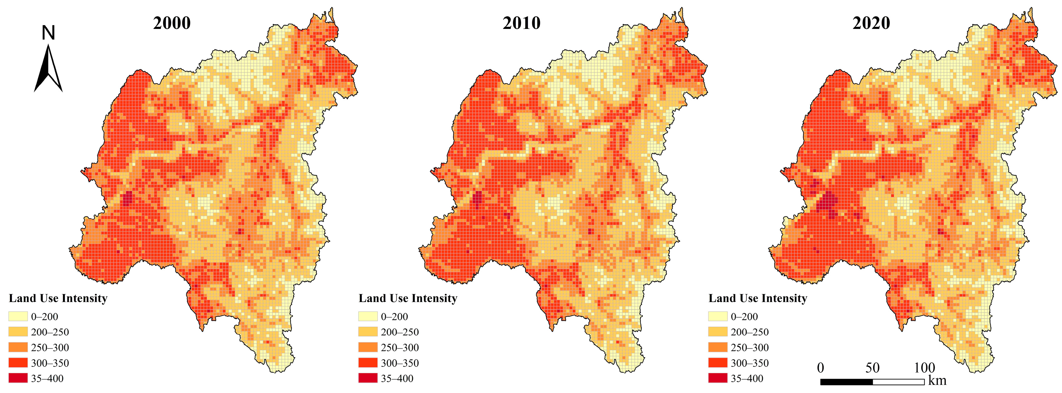
3.1. Changes in LUI during 2000–2020

Forest and agricultural land made up more than 80% of the total area of the land used for land use types in Harbin (

Table 4. Land use transition matrix (km²).

Years	Types	Agriculture Land	Forest	Grassland	Wetland	Water Body	Construction Land	Bare Land	Total
2000–2010	Agriculture land	26,010.70	311.72	468.93	6.78	56.47	273.00	0.10	27,127.68
	Forest	224.17	17,868.14	694.83	3.54	39.44	11.52	0	18,841.63
	Grassland	350.91	445.27	3112.82	32.41	85.51	99.83	0.01	4126.76
	Wetland	31.91	19.16	70.33	691.89	32.61	0.24	0	846.14
	Water body	71.60	22.95	26.88	11.16	473.16	0.76	0	606.52
	Construction land	266.69	14.65	57.64	0.07	1.53	1168.67	0	1509.26
	Bare land	0.0036	0.0009	0.01	0	0	0	0.02	0.03
2010–2020	Agriculture land	24,972.92	644.56	405.91	161.12	91.81	669.29	11.58	26,957.19
	Forest	286.71	17,397.62	872.70	30.97	35.96	59.77	0.85	18,684.58
	Grassland	321.87	950.90	2884.56	94.29	82.25	94.40	3.72	4431.98
	Wetland	14.33	0.16	5.90	594.66	126.44	4.43	0	745.93
	Water body	47.19	20.32	12.54	24.18	582.59	2.36	0.01	689.18
	Construction land	167.61	4.44	13.13	0.83	2.13	1365.17	0.72	1554.03
	Bare land	0.02	0.0045	0.05	0	0	0	0.06	0.12
2000–2020	Agriculture land	24,619.39	796.67	651.25	159.99	115.99	772.89	11.51	27,127.68
	Forest	353.66	17,341.01	999.92	30.86	56.13	59.22	0.83	18,841.63
	Grassland	463.11	832.77	2465.07	117.01	100.42	144.65	3.74	4126.76
	Wetland	42.27	13.27	22.00	576.09	187.45	5.07	0	846.14
	Water body	81.19	20.48	20.71	21.36	458.24	4.47	0.07	606.52
	Construction land	249.84	11.10	35.41	0.58	2.45	1209.12	0.76	1509.26
	Bare land	0.0027	0	0.01	0	0	0	0.02	0.03
	Total	25,809.46	19,015.30	4194.37	905.89	920.68	2195.42	16.93	53,058.02

). The western portion of the city was primarily made up of agricultural areas, whereas the northern and eastern portions of the city were heavily covered in forest. All other land use types accounted for less than 10% of the area. Almost every pair of land use types experienced land conversion from 2000 to 2020. The most significant was the conversion of forest to grassland, with 694.83 and 872.70 km² of forest converted to grassland in 2000–2010 and 2010–2020, respectively. This was followed by the conversion of grassland to forest (832.77 km²) and agricultural land to forest (796.67 km²), and then by the conversion of agricultural land to construction land (772.89 km²).

Figure 2 depicts the LUI in Harbin City in 2000, 2010, and 2020. The LUI space had a general pattern of “high in the west and low in the east”. With average values of 255.60 in 2000, 255.46 in 2010, and 255.58 in 2020, with a few minor changes, the average value of LUI from 2000 to 2020 exhibited a trend of dropping and then increasing. The low-LUI zones were mainly located in Tonghe County, Fangzheng County, Shangzhi City, and the southern part of Wuchang City, where there was a high coverage of forest and a low degree of interference from human activities, and thus the LUI was relatively low. The high-LUI zones were mainly concentrated in the built-up areas of the city and were most obvious in the areas with a high level of urbanization in the counties and districts. The medium-LUI zones were concentrated in the western part and the agricultural land in the southeastern corner of the city, which accounted for nearly 50% of the total area of Harbin City, and they were highly influenced by human activities and had certain natural attributes.

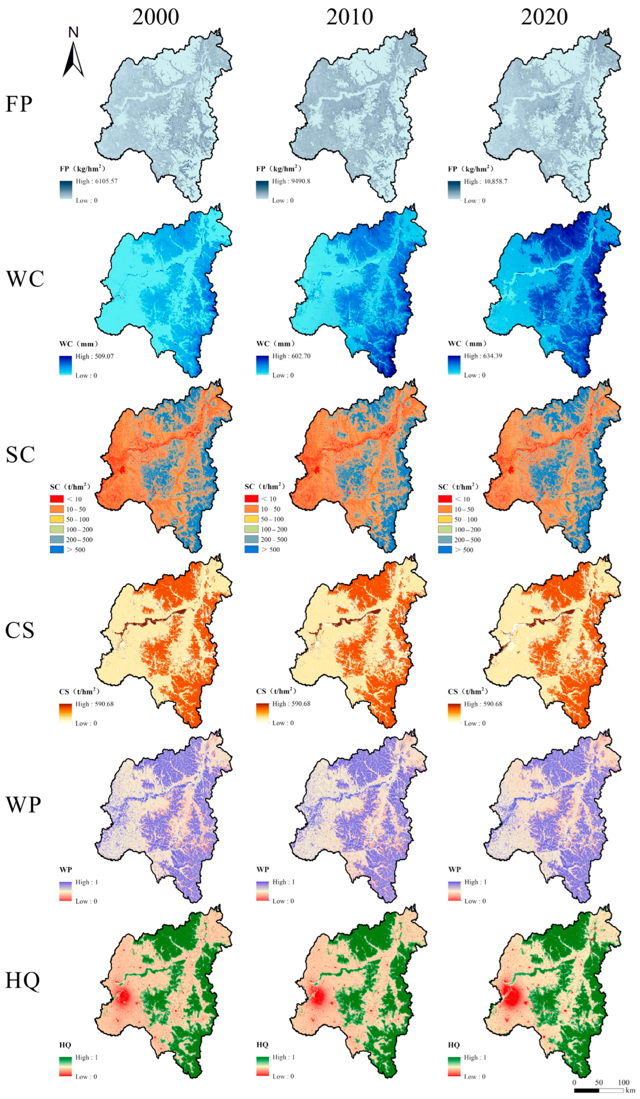
3.2. Changes in ESs during 2000–2020

From 2000 to 2020, Harbin City’s ESs had substantial changes (Figure 3). Except for FP, which showed a pattern of “high in the west and low in the east”, all other ESs showed a geographical distribution pattern of “low in the west and high in the east”. In 2000, 2010, and 2020, the overall quantities of FP were 6.95 × 10⁶ t, 1.26 × 10⁷ t, and 1.22 × 10⁷ t, respectively. The amount of FP per unit area was 1310.05 kg/hm², 2372.98 kg/hm², and 2304.65 kg/hm², respectively. The western part of the city, where agricultural land was the dominant land use type, had a high FP, whereas the Zhangguangcai Range and Xiaoxing’an Mountains’ ecological barrier area located in the east, where there was less human interference and where forest was the dominant land use type, had a low FP.

In 2000, 2010, and 2020, the average depths of WC were 58.07 mm, 130.40 mm, and 239.92 mm, respectively, showing a significant upward trend, and WC increased significantly from 3.08 × 10⁹ m³ in 2000 to 12.73 × 10⁹ m³ in 2020. From the perspective of spatial distribution, Harbin City’s distribution of WC in 2000, 2010, and 2020 was more constant, presenting an overall “west low east high” spatial distribution pattern. With an average depth of less than 200 mm, the low-WC areas were mostly found in urban areas, Bayan County in the west, and Bin County in the center, whereas the high-WC areas were mostly found in Tonghe County in the north, Fangzheng County, and Shangzhi City in the east, with an average depth of more than 300 mm.

In 2000, 2010, and 2020, SC decreased from 2.18 × 10⁹ t to 2.07 × 10⁹ t and then increased to 2.77 × 10⁹ t. Western urban areas, where agricultural land and construction land are the main land use types, had lower SC intensity, while the Zhangguangcai Range ecological barrier area, where forest was the main land use type, as well as Xiaoxing’an Mountains ecological barrier area, had significantly higher SC.

The overall trend of CS in Harbin City during 2000–2020 was relatively smooth and fluctuating, with unit area averages of 258.00 t/hm², 256.42 t/hm², and 257.10 t/hm², respectively, with no significant changes in the districts and counties, and both decreases and increases were small. The northern, central, and eastern parts of the city were located in the zone of high CS values, while the western part of the city was located in the zone of low values.

The back-normalized nitrogen output served as the WP index, and regions with higher nitrogen output had weaker WP. WP was measured using nitrogen output capacity as a negative indicator. The total nitrogen output was 1.35 × 10⁷ kg, 1.32 × 10⁷ kg, and 1.34 × 10⁷ kg, respectively, with nitrogen output intensities of 2.70 kg/hm² in 2000, 2.64 kg/hm² in 2010, and 2.68 kg/hm² in 2020. The general downward trend in nitrogen output meant that Harbin City’s WP was increasing.

From 2000 to 2020, habitat quality showed an overall upward trend, with an average value of 0.7215 in 2000 and 0.7279 in 2020, an increase of 0.89% in 2020 compared to 2000, with smaller fluctuations in all districts and counties. From a spatial point of view, the western built-up area was located in the low-value zone and had a continuing trend of expansion, posing a serious threat to the surrounding ecological environment.

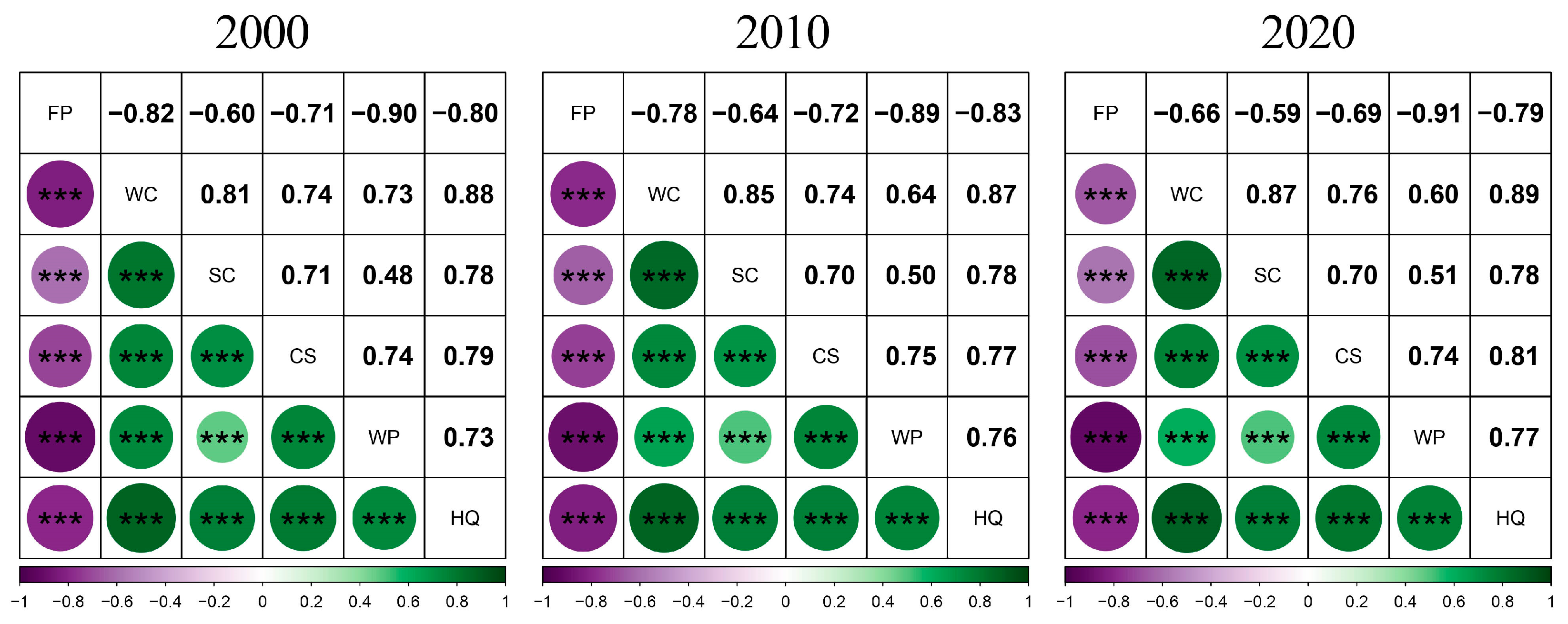
3.3. Spearman’s Correlation Analysis

On the 3 km × 3 km grid, the six major ESs in Harbin City from 2000 to 2020 displayed statistically significant associations (Figure 4). FP showed significant negative correlations with the other five ESs, and the degree of trade-offs decreased year by year. The other five ESs showed significant positive correlations with each other, where the degree of synergy between WC and SC increased year by year, while the degree of synergy between WC and WP decreased year by year.

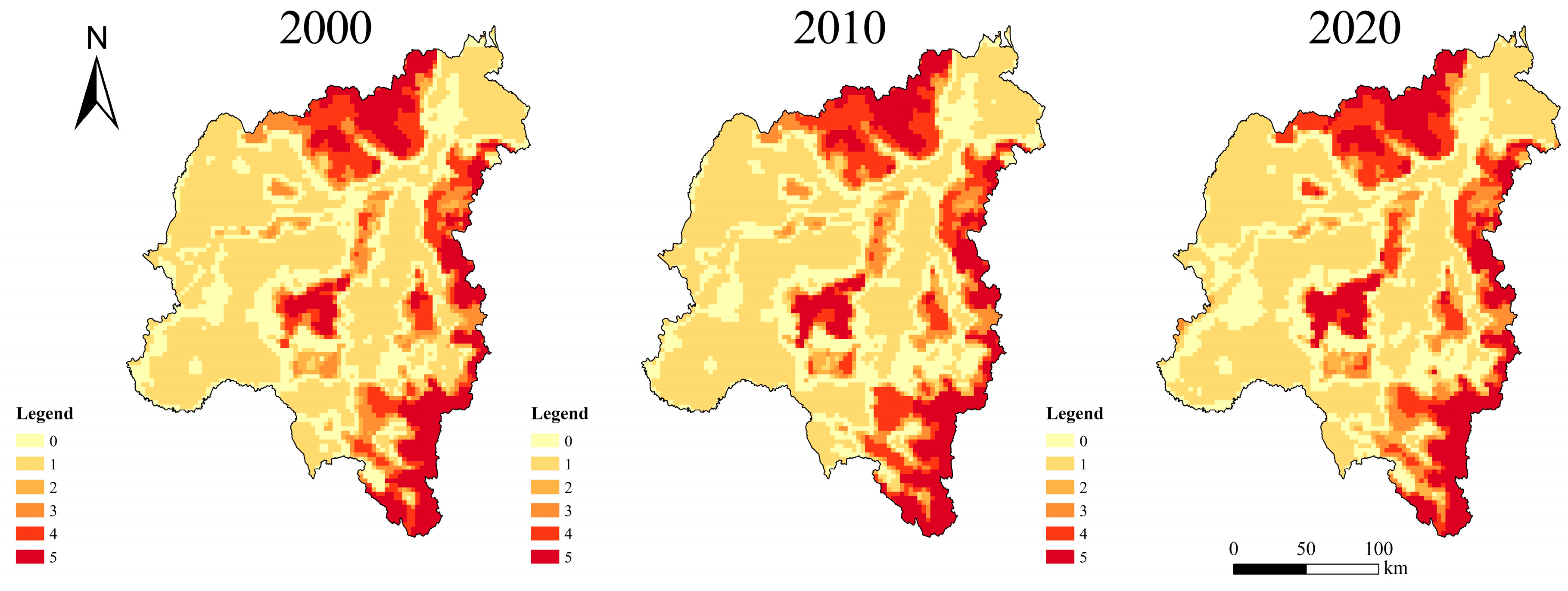
3.4. Identification of ES Hotspots

The hotspot area overlay analysis can reflect the comprehensive strength of ESs. The highest number of hotspots in Harbin is five, indicating that no region has all six ESs in the high-value area (Figure 5,

Table 5. Number of hotspots in different years in Harbin.

Hotspot Value	Area (km2)			Share (%)
	2000	2010	2020	2000	2010	2020
0	11,797.40	11,929.00	11,872.40	22.23	22.48	22.37
1	23,427.40	22,951.00	22,504.70	44.14	43.24	42.40
2	2289.40	2484.19	2428.52	4.31	4.68	4.58
3	3884.24	3422.17	3460.84	7.32	6.45	6.52
4	4855.82	5377.83	5182.12	9.15	10.13	9.76
5	6820.19	6910.29	7625.89	12.85	13.02	14.37

). The hotspots of ESs are mainly concentrated in the north and east side of the city, which are located in the area of high topographic relief, showing a contiguous distribution. The area of the level five hotspot area is increasing year by year, from 12.85% in 2000 to 14.37% in 2020, indicating that the area of the comprehensive high-value area of ESs is expanding in favor of the development of ESs. It shows that the area of the comprehensive high-value area of ESs is expanding, which is favorable for the ecological environment development of Harbin City.

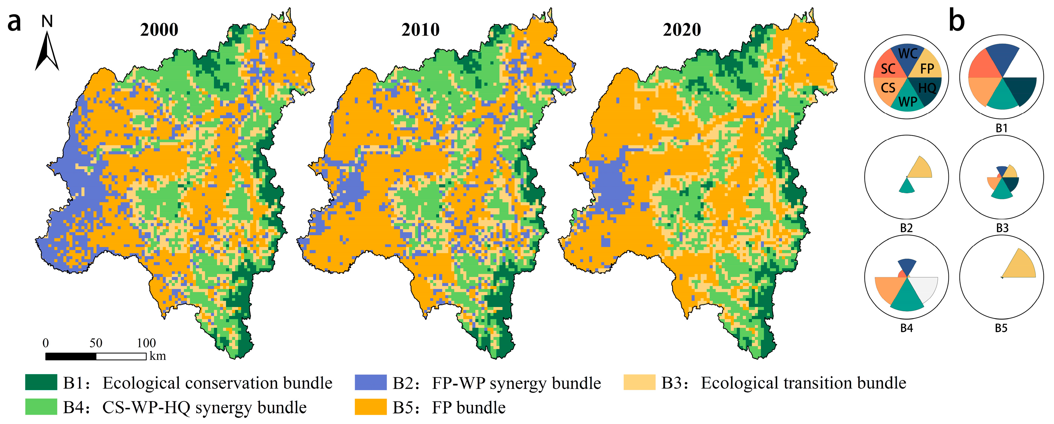
3.5. Spatial–Temporal Patterns of ES Bundles

In this study, five types of ES bundles in Harbin City were identified based on a 3 km × 3 km grid using the “kohonen” package in R (Figure 6). Different ES bundles reflect different ES aggregation characteristics. Within each cluster, a larger percentage of a given ES area represents a higher mean value within the corresponding grid (Figure 6b). According to the distribution features of each ES bundle, the bundles were termed the ecological conservation bundle (B1), FP–WP synergistic bundle (B2), ecological transition bundle (B3), CS–WP–HQ synergistic bundle (B4), and FP bundle (B5). B1 stands for high levels of all ESs except FP. B2 represents the ES bundle with high mean values of FP and WP. B3, on the other hand, represents a more balanced set of ESs, with no one ES being more prominent. B4 denotes ES bundles with high values of CS, WP, and HQ and low values of the other ESs. B5 indicates the ES bundle with high values of FP.

In B1, the types of ESs were primarily characterized by WC, SC, CS, WP, and HQ. FP was virtually nonexistent in this cluster. This bundle offered significant ecological value, which was consistent with the conditions typical of forest use types. B1 was mainly concentrated in the northern and eastern parts of the city, covering a smaller proportion of the area. B2 was primarily characterized by FP and WP as the main types of ESs. It not only boasted a significant capacity for food supply but also exhibits a robust capability for water quality purification. B2 was primarily concentrated in the agricultural areas surrounding the developed regions in the western part of the city. B3 exhibited a balanced distribution of ESs, possessing a certain ecological value. It was primarily located in the transitional areas between forests and agricultural lands. B4 was characterized mainly by CS, WP, and HQ and was concentrated in the ecological barrier zones of the Xiaoxing’an Mountains and Zhangguangcai Range. B5, on the other hand, was dominated by extensive agricultural lands in the western part of the city, boasting a very high food provision capacity.

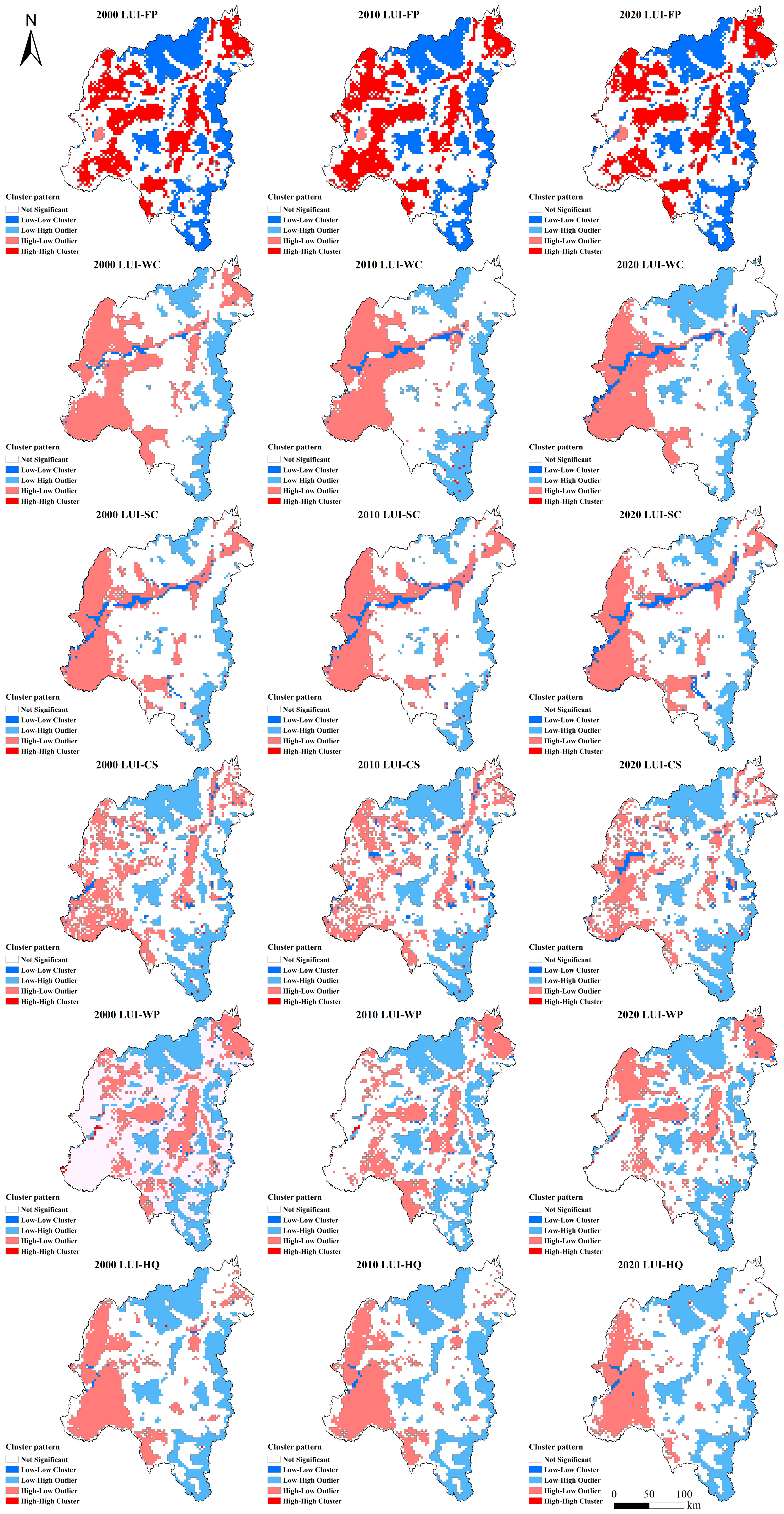
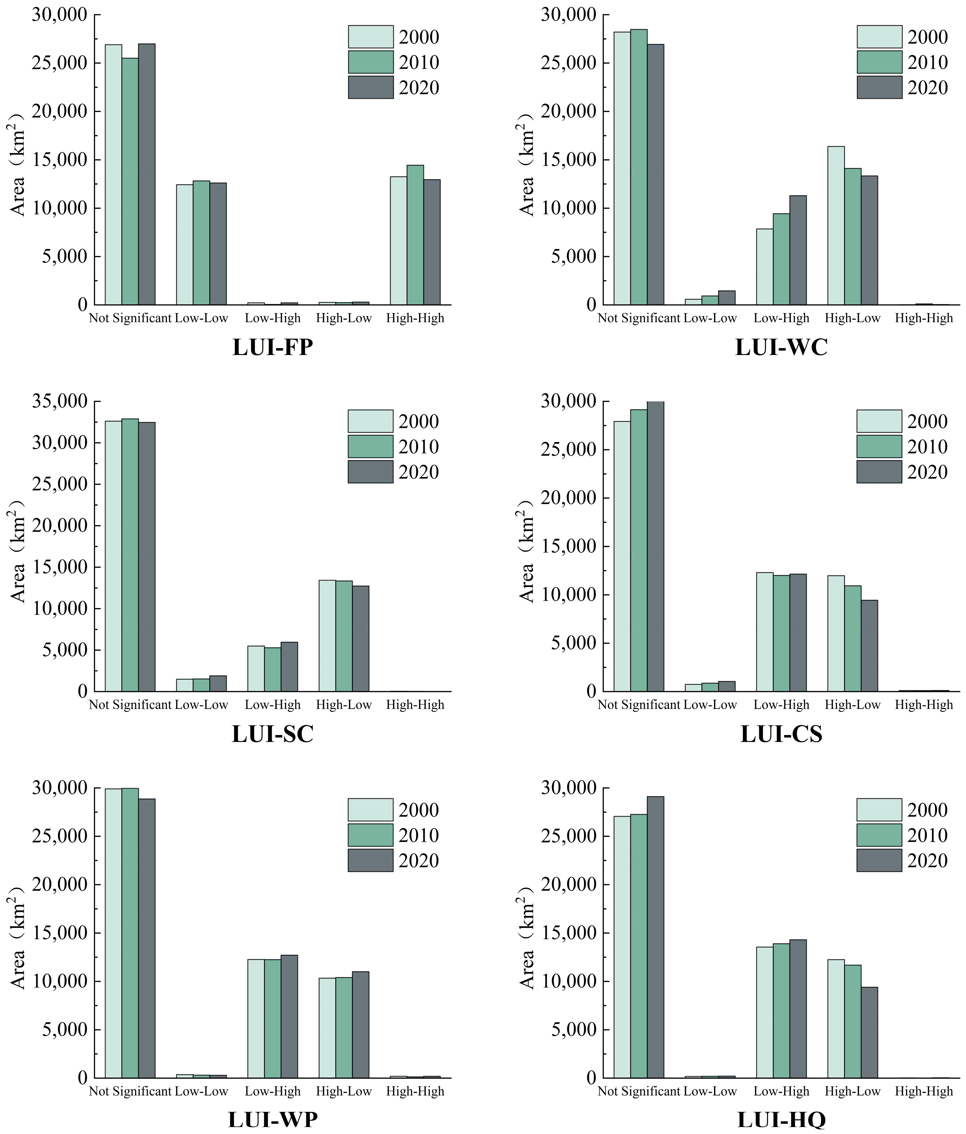
3.6. Impacts of LUI Changes on ESs

To further explore the influence of LUI on ESs, this study introduces a bivariate spatial autocorrelation model. The higher the LUI, the bigger the degree of influence of human activities on ESs.

Table 6. Global Moran’s I of LUI and ESs in different years.

Years	LUI-FP	LUI-WC	LUI-SC	LUI-CS	LUI-WP	LUI-HQ
2000	0.758	−0.763	−0.587	−0.750	−0.661	−0.845
2010	0.777	−0.780	−0.571	−0.742	−0.669	−0.847
2020	0.728	−0.765	−0.586	−0.718	−0.683	−0.847

displays the worldwide Moran index for the years 2000, 2010, and 2020; at this stage, p = 0.001 passes the significance test, suggesting a significant association between the LUI and the ESs. Apart from a positive correlation with FP, LUI was significantly negatively correlated with other ESs (ecosystem services). This meant that the stronger the LUI, the lower the level of ESs. Moreover, the negative correlation between the two is relatively stable, without evident changes in intensity.

The bivariate local spatial autocorrelation is shown in Figure 7. From 2000 to 2020, there were two significant spatial clustering types between LUI and FP in Harbin City, namely “Low LUI-Low FP” and “High LUI-High FP”. The “High LUI-High FP” was primarily located in the western part of the city, while “Low LUI-Low FP” was mainly concentrated in the northern and eastern parts of the city. Apart from FP, the relationship between LUI and other ESs was mainly characterized by the clustering types of “Low LUI-High ESs” and “High LUI-Low ESs”, while the proportions of “Low LUI-Low ESs” and “High LUI-High ESs” were relatively smaller.

“Low LUI-High WC”, “Low LUI-High SC”, “Low LUI-High CS”, and “Low LUI-High HQ” were mainly concentrated in the north and east of the study area, located inside the ecological barriers of Zhangguangcai Range and Xiaoxing’an Mountains. The lower LUI represented a lower degree of human disturbance, and its natural ecosystem was less affected and had higher Ess. While “High LUI-Low CS” displayed erratic distribution in the western part of the city, “High LUI-Low WC”, “High LUI-Low SC”, and “High LUI-Low HQ” were primarily concentrated in the western part of the city and displayed a continuous distribution. The land use type was dominated by construction land and agricultural land, which were more affected by human activities, and the stronger human activities seriously affected the function of the Ess, causing their WC and SC to be greatly reduced. With rare dispersal in other locations, “Low LUI-High WP” was mostly found in the city’s southeast and center. The “High LUI-Low WP” exhibited a consistent concentration in the city’s northern region, but it was dispersed over all districts and counties.

Figure 8 displays the areas of various spatial aggregation forms between LUIs and Ess. The results demonstrated that from 2000 to 2020, the areas of “Low LUI-Low FP” and “High LUI-High FP” both had a tendency of “first increasing and then declining”, and the area of the “High LUI-High FP” aggregation type was consistently higher than that of “Low LUI-Low FP”. The area share of “Low LUI-High WC” showed an increasing trend from 14.81% to 21.29%, while the area share of “High LUI-Low WC” decreased from 30.88% in 2000 to 25.14% in 2020, indicating that the water conservation capacity of Harbin City has been increasing in recent years, and the interference of LUI on WC has decreased. While the area of “high LUI-low SC” fell from 13,427.17 km² in 2000 to 12,728.19 km² in 2020, the area of “low LUI-high SC” showed a declining and then increasing trend, showing that Harbin City’s soil and water management has received positive feedback. The area of “Low LUI-High CS” decreased and then increased, while the area of “High LUI-Low CS” continued to decrease.

“Low LUI-High WP” showed a trend of “decreasing and then increasing”, decreasing from 12,271.30 km² to 12,251.17 km² in 2000, and then increasing to 12,710.84 km² in 2020, while the area proportion of “High LUI-Low WP” showed a continuous increase from 19.48% in 2000 to 20.74% in 2020. The percentage of the “High LUI-Low WP” area, on the other hand, showed a consistent rise from 19.48% in 2000 to 20.74% in 2020. As a significant “granary” for China, the annual application of massive amounts of chemical fertilizers has seriously harmed the ecosystem, and issues with water quality have become worse [45,59]. The area of “Low LUI-High HQ” kept growing, but the area of “High LUI-Low HQ” kept shrinking. This demonstrated that habitat quality in Harbin City was improving and that human disturbance activities had decreased, leading to a decline in habitat quality damage.

4. Discussion

4.1. Spatial Pattern and Evolution Characteristics in LUI and ESs

During the study period, different land use types demonstrated a complex two-way conversion between them. Influenced by the reform and opening-up policy and the policy of revitalizing the old industrial bases in Northeast China, urbanization and industrialization have continued to advance, and the area of land used for construction in Northeast China has expanded rapidly [60,61]. The FP displayed a geographic distribution pattern of “high in the west and low in the east” in the years 2000, 2010, and 2020, but the other ESs displayed a pattern of “low in the west and high in the east.” This is because ESs are impacted by a variety of causes, including alterations in land use, disturbance from people, and climate change [62]. Forest, grassland, and wetland generally have high ESs because they are less exposed to human disturbance activities, store large amounts of carbon, are rich in biodiversity, and are ideal environments for plants and animals [63,64]. Construction land and bare land have poorer ESs because rapid urbanization and industrialization are often accompanied by environmental degradation [65].

FP shows a distribution pattern of “high in the west and low in the east”, which is related to the land use structure of Harbin City. The western part of the city is dominated by agricultural land, which serves the function of food production, and thus has a higher FP. In addition to FP, other ES low-value areas are mainly located in the western part of the city. The main reason for this is that the land use type in this area is dominated by construction land and agricultural land, which is more affected by human interference, with lower vegetation cover, less interception of precipitation, and flatter topography, so the integrated ESs are weaker. This is consistent with the experience of previous studies [57,66,67]. The areas with high values of composite ESs are mainly located near the ecological barriers of Zhangguangcai Range and Xiaoxing’an Mountains, where forest, as the main land use type, has a high CS. This area has high vegetation cover, which has a strong saving effect on precipitation, coupled with a layer of deadfall that increases surface roughness, thus slowing down the rate of surface runoff, resulting in a high WC, and this result is consistent with previous studies [13,28]. At the same time, this area is in good SC and HQ condition due to its high elevation, high degree of topographic relief, and low intensity of anthropogenic disturbance.

The high-value areas of nitrogen output are located in Bayan, Yilan, and Bin counties. Because of its role as an important commercial grain base, a place of human long-term agricultural activities, the growth of crops grown on agricultural land has long depended on the use of pesticides and fertilizers, and most of them enter the surrounding water bodies with irrigation drainage and precipitation surface runoff, becoming the main source of nitrogen output, which has a significant impact on water quality. The 13th Five-Year Plan for the Revitalization of Northeast China (2016–2020), issued by the National Development and Reform Commission in 2016, advocates for the implementation of green production and lifestyle and the strengthening of pollution prevention and control. With the increase in environmental regulation, the water quality in the northeast region is on an improving trend [68].

4.2. Impact of LUI on ESs

The structure and function of ESs are impacted by the complex effects of land use change [69]. To explore the relationship between LUI and ESs, previous studies have focused more on quantifying the quantitative relationship between the two by using the land transfer matrix and simple statistical correlation [60], but they lacked the consideration of the spatial relationship. This study explores the influence of LUI on ESs from a spatial perspective, which is of great significance for scientific and rational spatial planning of land in the study area.

LUI in Harbin City seriously affects ESs. In 2000–2020, LUI showed a significant positive correlation with FP and a significant negative correlation with other ESs. A large number of studies have found that as LUI increases, provisioning services tend to increase while regulating or supporting services tend to decrease [18,70]. The present study verifies this observation. The areas of “High LUI-Low WC”, “High LUI-Low SC”, “High LUI-Low CS”, and “High LUI-Low HQ” all showed a continuous decreasing trend. The main reason is that a large amount of agricultural land has been converted to forest in the past 20 years, and the LUI has decreased, which has a positive impact on WC, CS, SC, and HQ. In addition, in recent years, the city has carried out a series of ecological protection plans and policies, such as the “Green Shield” and special operations to combat the destruction of wetland resources, and the return of agricultural land to forest, which, to a large extent, have contributed to the benign development of natural ecosystems and have served as a meaningful protection of land resources in the region.

Agricultural land in Harbin accounts for nearly 50% of the city’s total area and has natural attributes compared to urban ecosystems that are entirely dominated by humans, but compared to forest ecosystems, which are virtually unaffected by human activities, it is largely subject to a greater degree of human interference. The use of large quantities of pesticides and fertilizers and the discharge of household waste in the city have resulted in serious pollution of soil and water quality. Despite the fact that the agricultural pollution in Harbin City is still serious and the “High LUI-Low WP” is continuously increasing [38,71], it is urgent to improve the WP.

Therefore, in order to protect the ecological environment of Harbin City and improve its ESs, the management of land conversion should be strengthened and the transfer of land from areas with high ESs to areas with low ESs should be reduced. Special attention should be paid to strengthening the implementation of ecological projects during the development of agriculture and industry to prevent environmental degradation caused by over-exploitation.

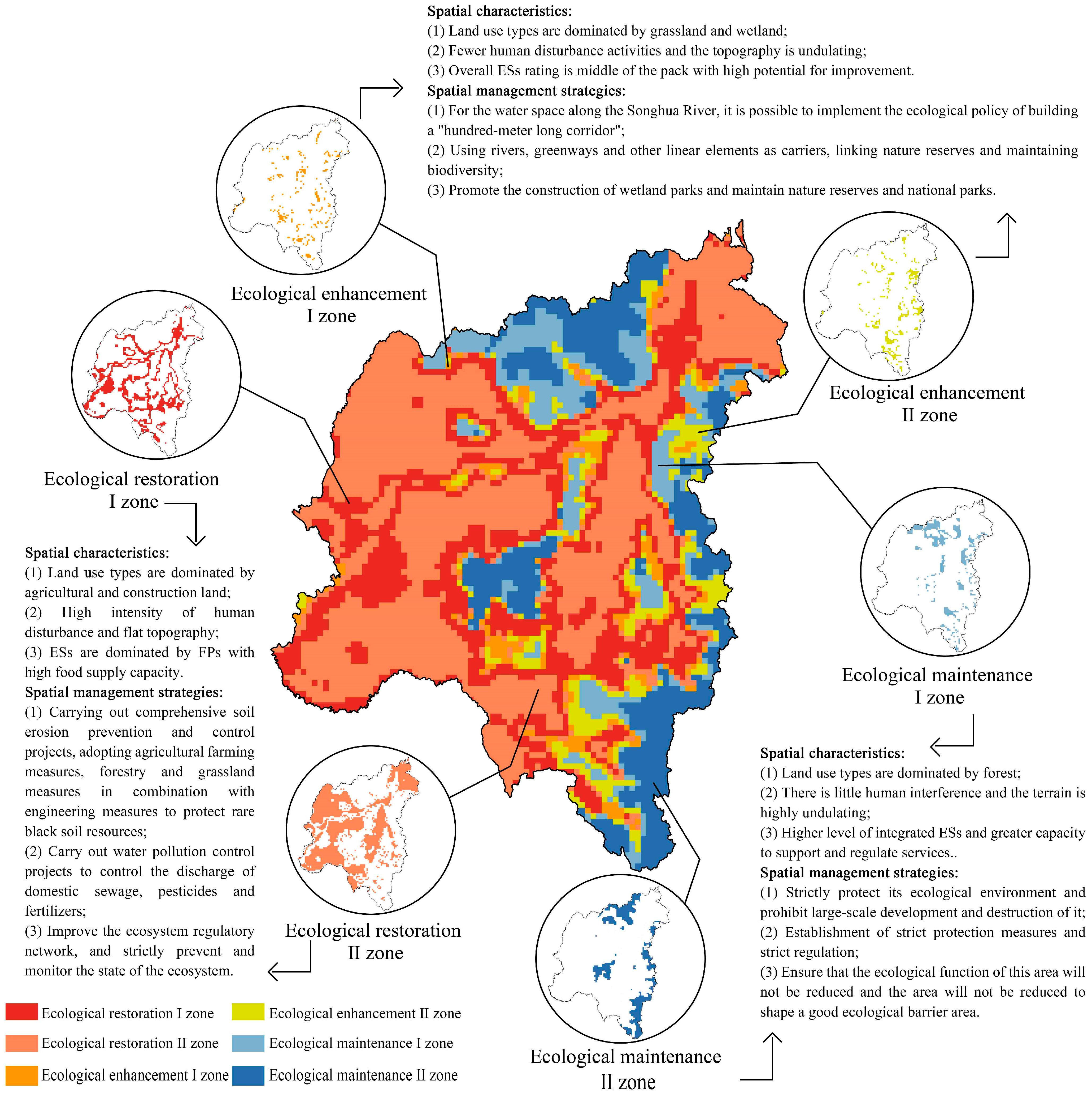
4.3. Policy Implications

The contribution of natural ecosystems to human society is irreplaceable, and ecosystem services are the vehicle for spatial planning for natural resource value shaping [72]. The spatial distribution pattern of ESs in Harbin City from 2000 to 2020 and the relationship with its LUI can provide a scientific reference basis for urban territorial spatial planning to cope with possible strategic issues raised in the introduction.

For the enhancement of integrated ESs, this study divides the territorial space into ecological restoration Ⅰ, ecological restoration Ⅱ, ecological enhancement Ⅰ, ecological enhancement Ⅱ, ecological maintenance Ⅰ, and ecological maintenance Ⅱ zones according to the hotspot area class (Figure 9), corresponding to hotspot grades from 0 to 5. Different ecological management strategies are proposed according to different ecological function zones. Policymakers can focus on the western part of the city as an FP maintenance area and a priority treatment area for WC and SC and carry out WC upgrading and erosion control to reduce the use of pesticides and fertilizers and protect the rare black soil layer. For food-rich regions, an appropriate increase in ecological land use is conducive to the promotion of regulating services [73]. The ecological barriers of Xiaoxing’an Mountains and Zhangguangcai Range are regarded as key protection zones for ESs, and relevant policies and regulations are introduced to strictly control the impacts of human disturbance activities to avoid reducing their ESs. At the same time, because farming, planting, and human daily life all affect WP, water quality pollution should be controlled in an integrated manner, and pollutant management should be strengthened and intensified in rural living areas. The use of green organic fertilizers should be promoted in the planting industry, while the management of excreta pollution from the cultivation industry should be intensified [38]. Carrying out wetland development, protection, and management projects along the Songhua River; focusing on the rare value of wetland; focusing on the protection of wetland ecosystems; continuing to promote the ecological protection and high-quality development planning of the Songhua River Hundred Mile Corridor; and combining the spatial functional zoning of the national territory are necessary to enhance the sustainable development of ESs.

5. Conclusions

In this work, we used the InVEST model to quantify six important ESs in Harbin City in 2000, 2010, and 2020; the “kohonen” package of the R programming language to identify five important ecosystem service bundles; and bivariate spatial autocorrelation to examine the effects of LUI on ESs. The following are the primary conclusions:

(1)

The main land uses in Harbin were agricultural land and forest, with the area of agricultural land continuing to decrease. The area of forest and wetland showed a trend of decreasing and then increasing, the area of grassland increased and then decreased, and the area of water bodies, construction land, and bare land continued to increase. The overall LUI showed a spatial distribution pattern of “high in the west and low in the east”, and during the period of 2000–2020, land use in Harbin City experienced a more drastic change, with the overall LUI showing a trend of decreasing and then increasing.

(2)

Except for FP, all other ESs showed a similar spatial distribution pattern of “low west and high east”, with WC showing a continuous and significant increase. WC showed a continuous increase, and the increase was very significant. Nitrogen export intensity decreased slightly, so WP showed a slight upward trend, while SC showed a decreasing and then an increasing trend and CS and HQ were generally stable, with little change. Based on the dominant ecosystem service types, Harbin City can be categorized into five ecosystem service bundles.

(3)

There is a significant positive correlation between LUI and FP and a significant negative correlation with other ESs. “High LUI-High FP” is mainly located in the western part of the city. “Low LUI-High WC”, “Low LUI-High SC”, “Low LUI-High CS”, and “Low LUI-High HQ” were mainly concentrated in the ecological barrier areas of Xiaoxing’an Mountains and Zhangguangcai Range.

The study’s findings can aid in delineating the impact of LUI on ESs and offer Harbin City a logical and practical scientific foundation for land resource allocation and ecological conservation. In future studies, attempts will be made to predict future LUI and ESs to help urban planners better understand potential ecosystem service trends so that preventive management measures can be taken.

References

1. Costanza, R.; D’Arge, R.; de Groot, R.; Farber, S.; Grasso, M.; Hannon, B.; Limburg, K.; Naeem, S.; O’Neill, R.V.; Paruelo, J.; et al. The value of the world’s ecosystem services and natural capital. Nature 1997, 387, 253–260. [Google Scholar] [CrossRef]
2. Haberl, H.; Wackernagel, M.; Wrbka, T. Land use and sustainability indicators. An introduction. Land Use Policy 2004, 21, 193–198. [Google Scholar] [CrossRef]
3. Mooney, H.; Duraiappah, A.; Larigauderie, A. Evolution of natural and social science interactions in global change research programs. Proc. Natl. Acad. Sci. USA 2013, 110, 3665–3672. [Google Scholar] [CrossRef]
4. Wang, Y.; Zhao, J.; Fu, J.; Wei, W. Quantitative assessment of water conservation function and spatial pattern in Shiyang River basin. Acta Ecol. Sin. 2018, 38, 4637–4648. [Google Scholar]
5. Liu, Y.; Zhao, W.; Jia, L. Soil conservation service: Concept, assessment, and outlook. Acta Ecol. Sin. 2019, 39, 432–440. [Google Scholar]
6. Terrado, M.; Acuña, V.; Ennaanay, D.; Tallis, H.; Sabater, S. Impact of climate extremes on hydrological ecosystem services in a heavily humanized Mediterranean basin. Ecol. Indic. 2014, 37, 199–209. [Google Scholar] [CrossRef]
7. Guo, J.; Jiang, C.; Wang, Y.; Yang, J.; Huang, W.; Gong, Q.; Zhao, Y.; Yang, Z.; Chen, W.; Ren, H. Exploring ecosystem responses to coastal exploitation and identifying their spatial determinants: Re-orienting ecosystem conservation strategies for landscape management. Ecol. Indic. 2022, 138, 108860. [Google Scholar] [CrossRef]
8. Wang, P.; Wang, J.; Zhang, J.; Ma, X.; Zhou, L.; Sun, Y. Spatial-temporal changes in ecosystem services and social-ecological drivers in a typical coastal tourism city: A case study of Sanya, China. Ecol. Indic. 2022, 145, 109607. [Google Scholar] [CrossRef]
9. Bai, Y.; Zheng, H.; Ouyang, Z.; Zhuang, C.; Jiang, B. Modeling hydrological ecosystem services and tradeoffs: A case study in Baiyangdian watershed, China. Environ. Earth Sci. 2013, 70, 709–718. [Google Scholar] [CrossRef]
10. Li, J.; Xie, B.; Gao, C.; Zhou, K.; Liu, C.; Zhao, W.; Xiao, J.; Xie, J. Impacts of natural and human factors on water-related ecosystem services in the Dongting Lake Basin. J. Clean. Prod. 2022, 370, 133400. [Google Scholar] [CrossRef]
11. Sample, J.E.; Baber, I.; Badger, R. A spatially distributed risk screening tool to assess climate and land use change impacts on water-related ecosystem services. Environ. Modell. Softw. 2016, 83, 12–26. [Google Scholar] [CrossRef]
12. Vihervaara, P.; Rönkä, M.; Walls, M. Trends in ecosystem service research: Early steps and current drivers. Ambio 2010, 39, 314–324. [Google Scholar] [CrossRef] [PubMed]
13. Xia, H.; Yuan, S.; Prishchepov, A.V. Spatial-temporal heterogeneity of ecosystem service interactions and their social-ecological drivers: Implications for spatial planning and management. Resour. Conserv. Recycl. 2023, 189, 106767. [Google Scholar] [CrossRef]
14. Verhagen, W.; Van Teeffelen, A.J.A.; Baggio Compagnucci, A.; Poggio, L.; Gimona, A.; Verburg, P.H. Effects of landscape configuration on mapping ecosystem service capacity: A review of evidence and a case study in Scotland. Landsc. Ecol. 2016, 31, 1457–1479. [Google Scholar] [CrossRef]
15. Liu, L.; Liu, H.; Ren, J.; Bian, Z.; Ding, S. Research progress on the mechanism of ecosystem services generation. Chin. J. Appl. Ecol. 2017, 28, 2731–2738. [Google Scholar]
16. Zeng, Z.; Yang, H.; Ning, Q.; Tang, H. Temporal and spatial evolution of land use intensity and its impact on ecosystem services in Dongting Lake Zone. Econ. Geogr. 2022, 42, 176–185. [Google Scholar]
17. Felipe-Lucia, M.; Com, N.F.; Bennett, E. Interactions among ecosystem services across land uses in a floodplain agroecosystem. Ecol. Soc. 2014, 19, 360–375. [Google Scholar] [CrossRef]
18. Kindu, M.; Schneider, T.; Teketay, D.; Knoke, T. Changes of ecosystem service values in response to land use/land cover dynamics in Munessa–Shashemene landscape of the Ethiopian highlands. Sci. Total Environ. 2016, 547, 137–147. [Google Scholar] [CrossRef] [PubMed]
19. Allan, E.; Manning, P.; Alt, F.; Binkenstein, J.; Blaser, S.; Grassein, F.; Klaus, V.; Kleinebecker, T.; Morris, E.; Oelmann, Y.; et al. Land use intensification alters ecosystem multifunctionality via loss of biodiversity and changes to functional composition. Ecol. Lett. 2015, 18, 834–843. [Google Scholar] [CrossRef] [PubMed]
20. Xu, C.; Pu, L.; Zhu, M.; Li, J.; Chen, X.; Wang, X.; Xie, X. Ecological security and ecosystem services in response to land use change in the coastal area of Jiangsu, China. Sustainability 2016, 8, 816. [Google Scholar] [CrossRef]
21. Li, J.; Dong, S.; Li, Y.; Wang, Y.; Li, Z.; Li, F. Effects of land use change on ecosystem services in the China–Mongolia–Russia economic corridor. J. Clean. Prod. 2022, 360, 132175. [Google Scholar] [CrossRef]
22. Xin, X.; Zhang, T.; He, F.; Zhang, W.; Chen, K. Assessing and simulating changes in ecosystem service value based on land use/cover change in coastal cities: A case study of Shanghai, China. Ocean Coast. Manag. 2023, 239, 106591. [Google Scholar] [CrossRef]
23. Cai, Y.; Zhang, P.; Wang, Q.; Wu, Y.; Ding, Y.; Nabi, M.; Fu, C.; Wang, H.; Wang, Q. How does water diversion affect land use change and ecosystem service: A case study of Baiyangdian wetland, China. J. Environ. Manag. 2023, 344, 118558. [Google Scholar] [CrossRef]
24. Wang, Z.; Liu, S.; Li, J.; Pan, C.; Wu, J.; Ran, J.; Su, Y. Remarkable improvement of ecosystem service values promoted by land use/land cover changes on the Yungui Plateau of China during 2001–2020. Ecol. Indic. 2022, 142, 109303. [Google Scholar] [CrossRef]
25. Li, H.; Ye, C.; Hua, J. Impact of land use change on ecosystem service value in Nanchang City. Res. Soil Water Conserv. 2020, 27, 277–285, 293. [Google Scholar] [CrossRef]
26. Xia, H.; Kong, W.; Zhou, G.; Sun, O.J. Impacts of landscape patterns on water-related ecosystem services under natural restoration in Liaohe River Reserve, China. Sci. Total Environ. 2021, 792, 148290. [Google Scholar] [CrossRef]
27. Vigerstol, K.L.; Aukema, J.E. A comparison of tools for modeling freshwater ecosystem services. J. Environ. Manag. 2011, 92, 2403–2409. [Google Scholar] [CrossRef]
28. Bai, Y.; Ochuodho, T.O.; Yang, J. Impact of land use and climate change on water-related ecosystem services in Kentucky, USA. Ecol. Indic. 2019, 102, 51–64. [Google Scholar] [CrossRef]
29. Yohannes, H.; Soromessa, T.; Argaw, M.; Warkineh, B. Spatio-temporal changes in ecosystem service bundles and hotspots in Beressa watershed of the Ethiopian highlands: Implications for landscape management. Environ. Chall. 2021, 5, 100324. [Google Scholar] [CrossRef]
30. Yohannes, H.; Soromessa, T.; Argaw, M.; Dewan, A. Impact of landscape pattern changes on hydrological ecosystem services in the Beressa watershed of the Blue Nile Basin in Ethiopia. Sci. Total Environ. 2021, 793, 148559. [Google Scholar] [CrossRef]
31. Wang, Y.; Dai, E. Spatial-temporal changes in ecosystem services and the trade-off relationship in mountain regions: A case study of Hengduan Mountain region in Southwest China. J. Clean. Prod. 2020, 264, 121573. [Google Scholar] [CrossRef]
32. Liu, W.; Zhan, J.; Zhao, F.; Wang, C.; Zhang, F.; Teng, Y.; Chu, X.; Kumi, M.A. Spatio-temporal variations of ecosystem services and their drivers in the Pearl River Delta, China. J. Clean. Prod. 2022, 337, 130466. [Google Scholar] [CrossRef]
33. Pan, H.; Wang, J.; Du, Z.; Wu, Z.; Zhang, H.; Ma, K. Spatiotemporal evolution of ecosystem services and its potential drivers in coalfields of Shanxi Province, China. Ecol. Indic. 2023, 148, 110109. [Google Scholar] [CrossRef]
34. Wei, Q.; Abudureheman, M.; Halike, A.; Yao, K.; Yao, L.; Tang, H.; Tuheti, B. Temporal and spatial variation analysis of habitat quality on the PLUS-InVEST model for Ebinur Lake Basin, China. Ecol. Indic. 2022, 145, 109632. [Google Scholar] [CrossRef]
35. Cai, C.; Shang, J. Supply-demand level and development capability of Harbin urban ecosystem. Chin. J. Appl. Ecol. 2009, 20, 163–169. [Google Scholar]
36. Jin, H.; Li, S.; Wang, S. Impacts of climatic change on permafrost and cold regions environments in China. Acta Geogr. Sin. 2000, 55, 161–173. [Google Scholar]
37. Wang, N.; Zang, S.; Zhang, L. Spatial and temporal variations of spermafrost thickness in Heilongjiang province in recent years. Geogr. Res. 2018, 37, 622–634. [Google Scholar]
38. Yang, Y.; Meng, X. Study on emission characteristics of agricultural non-point source pollution in Heilongjiang. Ecol. Econ. 2018, 34, 184–190. [Google Scholar] [CrossRef]
39. Xie, L.; Yang, Z.; Cai, J.; Cheng, Z.; Wen, T.; Song, T. Harbin: A rust belt city revival from its strategic position. Cities 2016, 58, 26–38. [Google Scholar] [CrossRef]
40. Ma, L.; Li, B.; Liu, Y.; Sun, X.; Fu, D.; Sun, S.; Thapa, S.; Geng, J.; Qi, H.; Zhang, A.; et al. Characterization, sources and risk assessment of PM2.5-bound polycyclic aromatic hydrocarbons (PAHs) and nitrated PAHs (NPAHs) in Harbin, a cold city in Northern China. J. Clean. Prod. 2020, 264, 121673. [Google Scholar] [CrossRef]
41. Xiao, L.; Wang, W.; He, X.; Lv, H.; Wei, C.; Zhou, W.; Zhang, B. Urban-rural and temporal differences of woody plants and bird species in Harbin city, northeastern China. Urban For. Urban Green. 2016, 20, 20–31. [Google Scholar] [CrossRef]
42. Peng, S.; Ding, Y.; Liu, W.; Li, Z. 1 km monthly temperature and precipitation dataset for China from 1901 to 2017. Earth Syst. Sci. Data 2019, 11, 1931–1946. [Google Scholar] [CrossRef]
43. Peng, S.; Ding, Y.; Wen, Z.; Chen, Y.; Cao, Y.; Ren, J. Spatiotemporal change and trend analysis of potential evapotranspiration over the Loess Plateau of China during 2011–2100. Agric. For. Meteorol. 2017, 233, 183–194. [Google Scholar] [CrossRef]
44. Zhuang, D.; Liu, J. Study on the model of regional differentiation of land use degee in China. J. Nat. Resour. 1997, 12, 105–111. [Google Scholar]
45. Yang, S.; Bai, Y.; Alatalo, J.M.; Wang, H.; Jiang, B.; Liu, G.; Chen, J. Spatio-temporal changes in water-related ecosystem services provision and trade-offs with food production. J. Clean. Prod. 2021, 286, 125316. [Google Scholar] [CrossRef]
46. Zhou, W.; Liu, G.; Pan, J.; Feng, X. Distribution of available soil water capacity in China. J. Geogr. Sci. 2005, 15, 3–12. [Google Scholar] [CrossRef]
47. He, S.; Zhu, W.; Cui, Y.; He, C.; Ye, L.; Feng, X.; Zhu, L. Study on soil erosion characteristics of Qihe Watershed in Taihang Mountains based on the InVEST model. Resour. Environ. Yangtze Basin 2019, 28, 426–439. [Google Scholar]
48. Sheng, M.; Fang, H.; Sun, Y.; Guo, M. Analysis of factors affecting soil erosion and sediment yield at catchments in the black soil region of Northeast China. J. Shaanxi Norm. Univ. Nat. Sci. Ed. 2015, 43, 86–92. [Google Scholar]
49. Liu, M.; Zhang, H.; Ren, H.; Pei, H. Spatiotemporal Variations of the Soil Conservation in the Agro-pastoral Ecotone of Northern China Under Grain for Green Program. Res. Soil Water Conserv. 2021, 28, 172–178. [Google Scholar]
50. Yan, L.; Gong, J.; Xu, C.; Cao, E.; Li, H.; Gao, B.; Li, Y. Spatiotemporal variations and influencing factors of soil conservation service based on InVEST model: A case study of Miyun Reservoir upstream basin of Zhangcheng area in Hebei. J. Soil Water Conserv. 2021, 35, 188–197. [Google Scholar]
51. Tang, X.; Zhao, X.; Bai, Y.; Tang, Z.; Wang, W.; Zhao, Y.; Wan, H.; Xie, Z.; Shi, X.; Wu, B.; et al. Carbon pools in China’s terrestrial ecosystems: New estimates based on an intensive field survey. Proc. Natl. Acad. Sci. USA 2018, 115, 4021–4026. [Google Scholar] [CrossRef] [PubMed]
52. Ye, K.; Meng, F.; Zhang, L.; Yao, Z.; Xue, H.; Cheng, P.; Zhang, D. Spatial-temporal variation characteristics and source analysis of nitrogen pollution in the Songhua River Basin. Res. Environ. Sci. 2020, 33, 901–910. [Google Scholar]
53. Zheng, L.; Wang, Y.; Li, J. Quantifying the spatial impact of landscape fragmentation on habitat quality: A multi-temporal dimensional comparison between the Yangtze River Economic Belt and Yellow River Basin of China. Land Use Policy 2023, 125, 106463. [Google Scholar] [CrossRef]
54. Zhang, X.; Song, W.; Lang, Y.; Feng, X.; Yuan, Q.; Wang, J. Land use changes in the coastal zone of China’s Hebei Province and the corresponding impacts on habitat quality. Land Use Policy 2020, 99, 104957. [Google Scholar] [CrossRef]
55. Li, Y.; Zhang, L.; Qiu, J.; Yan, J.; Wan, L.; Wang, P.; Hu, N.; Cheng, W.; Fu, B. Spatially explicit quantification of the interactions among ecosystem services. Landsc. Ecol. 2017, 32, 1181–1199. [Google Scholar] [CrossRef]
56. Shen, J.; Li, S.; Liu, L.; Liang, Z.; Wang, Y.; Wang, H.; Wu, S. Uncovering the relationships between ecosystem services and social-ecological drivers at different spatial scales in the Beijing-Tianjin-Hebei region. J. Clean. Prod. 2021, 290, 125193. [Google Scholar] [CrossRef]
57. Shen, J.; Li, S.; Liang, Z.; Liu, L.; Li, D.; Wu, S. Exploring the heterogeneity and nonlinearity of trade-offs and synergies among ecosystem services bundles in the Beijing-Tianjin-Hebei urban agglomeration. Ecosyst. Serv. 2020, 43, 101103. [Google Scholar] [CrossRef]
58. Zhu, Z.; Alimujiang, K. Analysis and simulation of the spatial autocorrelation pattern in the ecosystem service value of the oasis cities in dry areas. J. Ecol. Rural Environ. 2019, 35, 1531–1540. [Google Scholar]
59. Wang, B.; Wang, Y.; Wang, S. Improved water pollution index for determining spatiotemporal water quality dynamics: Case study in the Erdao Songhua River Basin, China. Ecol. Indic. 2021, 129, 107931. [Google Scholar] [CrossRef]
60. Li, Q.; Zhang, X.; Liu, Q.; Liu, Y.; Ding, Y.; Zhang, Q. Impact of land use intensity on ecosystem services: An example from the agro-pastoral ecotone of central Inner Mongolia. Sustainability 2017, 9, 1030. [Google Scholar] [CrossRef]
61. Zhou, Y.; Gu, G.; Ren, Q.; Yang, J. Research on the relationship between business cycle and industrial fluctuations in northeast China based on complete ensemble empirical mode decomposition with adaptive noise. Complexity 2021, 2021, 8832201. [Google Scholar] [CrossRef]
62. Fang, J.; Song, H.; Zhang, Y.; Li, Y.; Liu, J. Climate-dependence of ecosystem services in a nature reserve in northern China. PLoS ONE 2018, 13, e192727. [Google Scholar] [CrossRef] [PubMed]
63. Escobar-Ocampo, M.; Castillo-Santiago, M.; Ochoa-Gaona, S.; Enríquez, P.; Sibelet, N. Assessment of habitat quality and landscape connectivity for forest-dependent cracids in the Sierra Madre del Sur Mesoamerican biological corridor, Mexico. Trop. Conserv. Sci. 2019, 12, 324260266. [Google Scholar] [CrossRef]
64. Fernández-Alonso, M.J.; Rodríguez, A.; García-Velázquez, L.; Dos Santos, E.; de Almeida, L.; Lafuente, A.; Wang, J.; Singh, B.; Fangueiro, D.; Durán, J. Integrative effects of increasing aridity and biotic cover on soil attributes and functioning in coastal dune ecosystems. Geoderma 2021, 390, 114952. [Google Scholar] [CrossRef]
65. Xu, L.; Chen, S.S.; Xu, Y.; Li, G.; Su, W. Impacts of land-use change on habitat quality during 1985–2015 in the Taihu Lake Basin. Sustainability 2019, 11, 3513. [Google Scholar] [CrossRef]
66. Zhang, J.; Guo, W.; Cheng, C.; Tang, Z.; Qi, L. Trade-offs and driving factors of multiple ecosystem services and bundles under spatiotemporal changes in the Danjiangkou Basin, China. Ecol. Indic. 2022, 144, 109550. [Google Scholar] [CrossRef]
67. Chen, T.; Feng, Z.; Zhao, H.; Wu, K. Identification of ecosystem service bundles and driving factors in Beijing and its surrounding areas. Sci. Total Environ. 2020, 711, 134687. [Google Scholar] [CrossRef] [PubMed]
68. He, G.; Wang, S.; Zhang, B. Watering down environmental regulation in China. Q. J. Econ. 2020, 135, 2135–2185. [Google Scholar] [CrossRef]
69. Wang, S.; Meng, W.; Jin, X.; Zheng, B.; Zhang, L.; Xi, H. Ecological security problems of the major key lakes in China. Environ. Earth Sci. 2015, 74, 3825–3837. [Google Scholar] [CrossRef]
70. Xu, Y.; Tang, H.; Wang, B.; Chen, J. Effects of land-use intensity on ecosystem services and human well-being: A case study in Huailai County, China. Environ. Earth Sci. 2016, 75, 416. [Google Scholar] [CrossRef]
71. Yue, Y.; Cheng, H.; Yang, S.; Hao, F. Integrated assessment of non-point source pollution in Songhuajiang River Basin. Sci. Geogr. Sin. 2007, 27, 231–236. [Google Scholar]
72. Li, R.; Li, Y.; Hu, H. Support of ecosystem services for spatial planning theories and practices. Acta Geogr. Sin. 2020, 75, 2417–2430. [Google Scholar]
73. Liang, J.; Li, S.; Li, X.; Li, X.; Liu, Q.; Meng, Q.; Lin, A.; Li, J. Trade-off analyses and optimization of water-related ecosystem services (WRESs) based on land use change in a typical agricultural watershed, southern China. J. Clean. Prod. 2021, 279, 123851. [Google Scholar] [CrossRef]
Figure 1. Location of the study area.
Sustainability 15 14877 g001
Figure 2. Spatial distribution pattern of LUI in different years in Harbin.
Sustainability 15 14877 g002
Figure 3. Spatial distribution pattern of ESs in different years in Harbin.
Sustainability 15 14877 g003
Figure 4. Trade-offs and synergies between pairs of ESs from 2000 to 2020. Notes: *** indicates significance at 0.001 probability levels.
Sustainability 15 14877 g004
Figure 5. Overlay map of hotspot areas.
Sustainability 15 14877 g005
Figure 6. (a) Spatial–temporal patterns of ES bundles. (b) Composition and relative magnitude of ESs in ES bundles. Longer segments represent higher ES supply.
Sustainability 15 14877 g006
Figure 7. Local spatial auto-correlation distribution of LUI and Ess in the study area in different years.
Sustainability 15 14877 g007
Figure 8. Local spatial autocorrelation type area for LUI and ESs.
Sustainability 15 14877 g008
Figure 9. Spatial management and planning strategies.
Sustainability 15 14877 g009