Analyzing Spatial Dependence of Rice Production in Northeast Thailand for Sustainable Agriculture: An Optimal Copula Function Approach

Abstract

Rice is not only central to Thailand’s economy and dietary consumption but also plays a significant role in global food security. Northeast Thailand, in particular, is a principal region for rice cultivation. However, with the mounting concerns of climate change, it becomes paramount to understand the interplay between regional weather patterns and rice yields, aiming to develop effective adaptive agricultural strategies. The current study aimed to fill the research gap by investigating an optimal copula for the spatial dependence of rice production and related meteorological variables in this area. The objective of this study is to understand how rice production in different areas relates to each other in order to improve farming practices and address challenges such as suitable weather. To achieve this goal, we apply three families of copulas—elliptical, Archimedean, and extreme—to analyze crop and meteorological variables across the watershed in the northeastern region of Thailand. With a data foundation extending from 1981 to 2021 from the Regional Office of Agricultural Economics Sector 4, Thailand, this study offers a comprehensive analysis of the spatial dynamics driving rice production across twenty provinces in Northeast Thailand. Using a piecewise linear model, we dissected rice yield trends, revealing distinct slopes in production and yield across various periods. The analysis leaned on elliptical, Archimedean, and extreme copula families, using the maximum likelihood estimation to discern marginal distribution residuals. Through rigorous bootstrap goodness-of-fit tests and cross-validation, the most appropriate copula for each province was identified. Key findings demonstrate pronounced spatial interdependencies in rice yields, with the Frank copula prominently capturing the product relationship between provinces such as Maha Sarakham and Roi-Et. Conversely, the Clayton copula better characterized regions such as Srisaket and Ubon Ratchathani. Moreover, the results underscore the considerable influence of meteorological factors, notably rainfall and temperature, on rice production, especially in regions like Ubon Ratchathani. In distilling these multifaceted relationships, the study charts a pathway for crafting sustainable, localized agricultural strategies. As the world grapples with climate change’s ramifications, the insights from this research stand crucial, offering direction for fostering resilience, adaptation, and optimizing rice productivity across Thailand’s diverse agrarian landscapes.

1. Introduction

By 2050, the world population is expected to increase to 10 billion people. Agricultural countries around the world are waking up to the need to produce enough food to meet the needs of the world’s population. Thailand is an agricultural country that has the opportunity to produce food for the world’s population [1], especially through rice production, which is the main food and contributes to the food security of the world’s population [2]. In 2022, Thailand exported 7.69 million tonnes of rice with an export value of USD 3.971 billion [3]. The type of rice that Thailand exports in large quantities is white rice, followed by Jasmine rice, Parboiled rice, Broken rice, Glutinous rice, and Brown rice [4]. In the 2020/2021 crop year, Thailand had a rice plantation area of 10.99 million hectares, and most rice plantations are located in the northeastern, lower northern, and central regions [4].

In 2022, Thailand was ranked as one of the top three rice-exporting countries in the world [3], but the yield of Thai rice is quite low when compared to the neighboring countries [5]. For example, rice yields per hectare in Vietnam are as high as 5.69 tons; at the same time, Thailand’s rice production is only 3.01 tons per hectare [2]. In Thailand, rice cultivation is generally carried out during the rainy season with a rain-fed system [6]. Factors affecting rice production in Thailand include climate change, soil fertility, soil quality, high cost of farm chemicals, and rising labor costs [5,6,7]. One of the main problems facing Thai farmers is rising production costs, but rice productivity is still low [5]. The cost of rice cultivation is expected to increase from 9831 THB/ton/year in 2021 to 10,500–11,000 THB/ton/year in 2024 [4].

Northeast Thailand is the main area of rice cultivation in Thailand [8]. Eighty percent of Northeast Thailand is an undulating plateau with extremely low soil fertility with a sandy texture and low water-holding capacity in the soil [6,9] In addition, the soil in the Northeast in some areas still faces the problem of saline soil which also affects rice productivity [10]. About 1.84 Mha of Northeast Thailand are affected by saline soils, including Nakhon Ratchasima, Khon Kaen, and Maha Sarakham province [11]. Saline soil distribution in Northeast Thailand is expected to increase in the future due to climate change [11,12]. All the problems mentioned above, combined with global climate change, will have a greater impact on agriculture worldwide. Facing a long drought due to global warming, Thai farmers need to adapt to farming that uses less water for sustainable farming [5]. Rice farming is very important for Thailand, especially in the Northeast. The current study aimed to fill the research gap by investigating an optimal copula for the spatial dependence of rice production and related variables in this area. To the best of our knowledge, rarely previous studies have been conducted on this specific type of data in Northeast Thailand. The objective of this study is to understand how rice production in different areas relates to each other in order to improve farming practices and address challenges such as suitable weather. Although there is a substantial amount of data available, a thorough investigation is still needed to comprehend how rice yields change over time, particularly in the context of climate change issues. To achieve this goal, we apply three families of copulas—elliptical, Archimedean, and extreme—to analyze crop and meteorological variables across the watershed in the northeastern region of Thailand.

The rest of this paper is organized as follows: Section 2 introduces the geographical region of interest for this research along with the data we have employed. An extensive overview of the materials and techniques utilized for this research is provided in Section 3. In Section 4, we discuss the outcomes of our research, with a particular emphasis on the spatial aspects and the performance of the copula models. Section 5 is devoted to an in-depth discussion of these findings, offers our conclusions and suggests recommendations based on our research.

2. Materials and Methods

2.1. Study Area

Northeast Thailand, located on the Khorat Plateau between the Phetchabun Range and the Mekong River, has varied terraces susceptible to droughts and floods, impacting their farming potential [13]. Typically, these lands are categorized into high, middle, and low terraces, each with distinct vulnerabilities to droughts and floods, affecting their suitability for cultivating rice and other field crops [14]. The majority of the plateau’s cultivable soils are sandy, acidic, and nutrient-poor, predominantly composed of quartz and kaolinite resulting from extensively weathered source materials. Additionally, regions, especially towards the west, face significant salt challenges, affecting agricultural productivity. Figure 1 shows land use map of the northeast region of Thailand as below:

2.2. Data

Thailand experiences three distinct seasons: the hot season (March to June), the rainy season (July to October), and the winter season (November to February). Each of these seasons can affect agricultural activities in Thailand, especially agriculture. For instance, rice farming is significantly influenced by the rainy season, which provides the necessary water for paddy fields, especially rain-fed paddy fields. In addition, the elevated nature of high terraces makes them more prone to droughts as water drains off quickly; middle terraces with their mid-level elevation have a mixed susceptibility to both droughts and occasional floods, while the low terraces, being closer to water sources, often grapple with frequent flooding and waterlogging [15].

In the Northeast, similar to other parts of the region, rice cultivation takes place in two primary seasons: the wet (WS) and dry (DS) seasons. The majority of the rice fields depend on rainwater, primarily produced during the WS, which spans from May to October. The DS spans from November to February. The disparity between these seasons is notably more pronounced in Northeast Thailand compared to other regions in mainland Southeast Asia [16]. Although rainfall during the WS can be unpredictable, it is often so abundant and frequent that it leads to localized flooding. Representing 46% of Thailand’s agricultural holdings and 47% of its farmable land, the Northeast boasts an average holding size of 3.2 hectare [17]. This research further delves into the attribute types, notation, and predictor variables, which are elaborated on in

Table 1. Attribute types, notation, and predictor variables.

Attribute Type	Attribute	Unit	Notation
Crops	cultivated area	hectare (ha)	CA
	harvested area	hectare (ha)	HA
	Productivity	ton	Product
	yield per rai	Kilogram (kg)	Yield
Meteorological variables	Average rainfall	mm.	Ave_rain
	Cumulative rainfall	Millimeter (mm)	sum_rain
	Average temperature	°C	Ave_tem
	Average relative humidity	%	Ave_rh

Note: Observational data from the Regional Office of Agricultural Economics 4 and the Thai Meteorological Department.

. For a detailed breakdown of cultivated and harvested areas, productivity, and yield rates for both the WS and DS in the Northeast from 1991–2021, see

Table 2. Average (with Standard Deviation) of cultivated area (1000 ha), harvested area (1000 ha), productivity (1000 ton), and yield per ha (1000 kg) for both wet (WS) and dry seasons (DS) in northeastern regions: data from selected years (1991–2021).

Province	Cultivated Area (1000 ha)		Harvested Area (1000 ha)		Productivities (1000 ton)		Rice Yield (1000 kg/ha)
	WS	DS	WS	DS	WS	DS	WS	DS
Loei	63.03 (8.59)	0.26 (0.20)	59.44 (9.14)	0.26 (0.20)	145.70 (23.87)	0.75 (0.62)	2.46 (0.42)	2.78 (0.29)
Nong Bua Lamphu	131.70 (15.93)	2.58 (2.29)	122.22 (15.93)	2.53 (2.24)	245.06 (36.95)	8.16 (7.75)	2.01 (0.48)	3.01 (0.18)
Udon Thani	343.60 (62.40)	5.74 (4.68)	323.83 (61.37)	5.65 (4.69)	594.18 (113.77)	16.32 (14.03)	1.89 (0.36)	2.77 (0.40)
Nong Khai	149.39 (41.40)	8.77 (5.61)	135.80 (36.55)	8.58 (5.58)	254.84 (60.16)	26.87 (19.19)	1.93 (0.40)	2.94 (0.29)
Beung Kan	80.06 (4.64)	1.89 (0.43)	72.96 (4.01)	1.85 (0.43)	144.78 (11.62)	5.89 (1.38)	1.99 (0.05)	3.18 (0.15)
Nakhon Phanom	177.07 (31.95)	5.74 (4.56)	161.75 (35.81)	5.58 (4.59)	305.63 (118.50)	15.97 (14.46)	1.84 (0.43)	2.61 (0.36)
Sakon Nakhon	285.71 (39.87)	5.74 (4.79)	266.95 (43.40)	5.61 (4.77)	498.75 (143.50)	16.25 (15.53)	1.84 (0.47)	2.56 (0.31)
Mukdahan	61.71 (11.46)	0.13 (0.11)	58.69 (11.58)	0.12 (0.11)	119.83 (40.91)	0.33 (0.30)	2.00 (0.48)	2.56 (0.35)
Amnat Charoen	153.29 (9.53)	0.47 (0.41)	146.66 (9.57)	0.46 (0.41)	290.51 (44.58)	1.32 (1.29)	1.98 (0.51)	2.58 (0.23)
Khon Kaen	337.23 (50.20)	17.57 (11.84)	301.86 (46.92)	17.17 (11.70)	574.82 (145.96)	57.69 (43.00)	1.88 (0.39)	3.24 (0.26)
Maha Sarakham	287.09 (46.29)	17.06 (12.05)	261.66 (43.39)	16.81 (11.88)	514.93 (165.13)	62.15 (46.16)	1.93 (0.29)	3.58 (0.39)
Roi Et	427.01 (51.46)	18.75 (16.54)	390.71 (44.30)	18.44 (16.26)	758.48 (215.67)	65.04 (58.38)	1.92 (0.43)	3.37 (0.41)
Kalasin	202.17 (32.47)	30.58 (16.42)	190.60 (30.67)	30.33 (16.41)	403.76 (102.12)	111.26 (65.00)	2.09 (0.42)	3.54 (0.28)
Yasothon	178.88 (23.82)	6.65 (7.48)	166.99 (20.81)	6.57 (7.35)	312.01 (93.54)	21.35 (24.29)	1.84 (0.39)	3.04 (0.38)
Chaiyaphum	215.43 (43.61)	8.09 (10.14)	188.72 (37.26)	7.99 (10.10)	381.36 (119.24)	26.64 (33.48)	1.98 (0.46)	3.13 (0.33)
Nakhon Ratchasima	499.14 (73.48)	18.95 (21.81)	446.72 (65.86)	18.60 (21.27)	851.80 (241.23)	69.48 (81.89)	1.88 (0.51)	3.44 (0.34)
Buriram	437.58 (36.53)	3.12 (4.74)	408.58 (39.62)	3.08 (4.67)	806.89 (180.42)	9.30 (14.46)	1.96 (0.49)	2.68 (0.34)
Surin	445.30 (60.76)	3.91 (5.25)	421.33 (57.23)	3.86 (5.19)	860.70 (229.94)	10.72 (15.07)	2.03 (0.41)	2.59 (0.38)
Sisaket	398.81 (62.36)	6.31 (6.12)	380.56 (62.19)	6.16 (5.93)	769.45 (235.29)	18.27 (18.86)	1.99 (0.48)	2.64 (0.38)
Ubon Ratchathani	567.08 (62.66)	14.49 (9.13)	541.65 (65.74)	14.38 (9.12)	959.87 (270.57)	37.69 (29.25)	1.76 (0.48)	2.37 (0.36)

.

For the WS, as observed in Table 2, Ubon Ratchathani, Nakhon Ratchasima, Surin, Burirum, and Roi-Et province rank in the top five in terms of cultivated area (1000 ha), harvest area (1000 ha), and productivity (1000 ton). However, they do not lead in terms of rice yield (1000 kg/ha). The top five provinces for rice yield (1000 kg/ha) include Loei, Kalasin, Surin, Mukdahan, and Nong Bua Lamphu, respectively. In contrast, for the DS, as indicated in Table 2, Kalasin, Nakhon Ratchasima, Roi Et, Khon Kaen, and Maha Sarakham province consistently dominate the top five positions for cultivated area (1000 ha), harvest area (1000 ha), productivity (1000 ton), and rice yield (1000 kg/ha). This underlines the need to investigate the weather’s impact on rice productivity across different regions. In this research, copula methodology has been chosen to analyze the correlations among these datasets. Additionally, trend analysis is employed to examine the association between predictor and outcome variables, especially when the relationship is not uniform across the entire predictor variable range. Figure 2 presents essential meteorological data for Northeast Thailand spanning the years 1981–2021. Among the regions studied, Nakhon Phanom registered the highest annual mean and cumulative rainfall (measured in mm). Nakhon Ratchasima exhibited the peak annual average temperature (in Celsius), while Kalasin recorded the maximum annual average relative humidity (expressed as a percentage).

2.3. Methodology

2.3.1. Trend Analysis

The segmented regression model, also referred to as a piecewise linear model, emerges as a powerful methodology to delineate the relationship between a predictor and its corresponding response variable, especially when this relationship does not maintain a constant presence throughout the predictor variable’s full range. At its core, this model fuses various linear segments that intersect at designated junctions, often labeled as breakpoints or knots. The foundational equation for a segmented regression model, characterized by a singular breakpoint, can be expressed via Equation (1):

$$Y_i={\beta }_0+{\beta }_1{X}_i+{\beta }_2(X_i-\tau )\times I(X_i>\tau )+{ϵ}_i.$$

(1)

Within this equation, $Y_i$ symbolizes the response variable, while $X_i$ stands for the predictor variable. $\tau$ designates the breakpoint, and $I\left(\right)$ acts as the indicator function (amounting to 1 when $X_i$ > $\tau$, and 0 in other scenarios). The parameters ${\beta }_0$, ${\beta }_1$, and ${\beta }_2$ are subject to estimation, and $E_i$ indicates the error term. Here, ${\beta }_1$ demarcates the line’s slope leading up to the breakpoint, while ${\beta }_1+{\beta }_2$ outlines the slope post-breakpoint. In essence, ${\beta }_2$ elucidates the shift in slope at the breakpoint’s location. These models extend a robust mix of adaptability and clarity, making them invaluable when dissecting intricate, non-linear data relationships, especially in contexts demanding the pinpointing of thresholds or breakpoints [18]. The chosen crop attributes serve as the response variable, while time (years) is used as the predictor variable.

A depiction of variations in rice yield spanning from 1981 to 2021, framed within dual productivity-area combinations during WS, accompanied by segmented regression lines for the Ubon Ratchathani province, can be observed in Figure 3. The analysis distinctly highlights two separate slopes in the production (ton) regression line (blue line)—one from 1921–2000 and the other from 2001–2021, both of which are on an upward trend. For the area (ha), there is a declining slope from 1921–2000, which reverses into an increasing trend from 2001 upwards. Notably, from 2015, both the production and area regression lines converge, indicating that as the area increases, production correspondingly rises.

2.3.2. Copula Function

Recently, the field of copulas has seen rapid advancements, demonstrating significant potential in analyzing multivariate joint distributions and conducting multivariate frequency assessments. The primary strength of copulas lies in their ability to capture the interdependence among variables, enabling the computation of joint probabilities without being affected by the marginal tendencies of the variables in question. Essentially, using copula functions seamlessly merges several univariate marginal distributions to generate their associated joint distribution. The copula function stands as a multivariate distribution where all its univariate margins align with $U(0,1)$. Considering a random vector $(X_1,\dots ,X_n)$, it is characterized by a joint distribution function $H(X_1,\dots ,X_n)$ and a continuous marginal distribution function $(F_i\left(X_1\right)=u_i)$. Here, $U_i$ possesses a uniform distribution over $[0,1]$ for $i=1,\cdots ,d$. Consequently, a unique d-dimensional copula C emerges [19,20,21,22]. In addition, the optimal copula function approach provides a comprehensive and flexible framework for understanding spatial dependencies, especially with its ability to capture diverse and non-linear relationships. Its strength lies in distinguishing marginal distributions and dependencies, as well as in capturing tail dependencies often overlooked by traditional methods. However, this approach can be computationally intensive, requires careful model selection, and may not inherently consider spatial continuity as efficiently as some geostatistical or Bayesian models. Although it offers advantages over deterministic and some stochastic methods in terms of flexibility and depth, the choice to use copulas should be based on the specific research objectives, data characteristics, and the need to model spatial continuity.

2.3.3. Copulas Families

Sklar’s theorem, proposed in 1959 by Sklar [21], describes the relationship between marginal distributions and heterogeneous distributions, known as the “copula”. Thus, any cumulative distribution function (CDF), $(F(X_1,X_2)$, of two random variables $(X_1,X_2)$ can be stated as Equation (2);

$$F(X_1,X_2)=C(F_1\left(x_1\right),F_2\left(x_2\right)),$$

(2)

where $F_1\left(x_1\right)$ and $F_2\left(x_2\right)$ are the marginal CDFs of variables $X_1$ and $X_2$, and C is a bivariate copula function.

Among all copula families, the elliptical copula family and the Archimedean copula family have been widely used in many areas. There is a variety of forms for both two copula families. In this study, the elliptical copulas (Normal copula and t copula), the Archimedes copulas (Clayton copula, Frank copula, and Joe copula) and the extreme value copula (Gumbel copula, Gumbel–Hougaard copula, and Husler–Reiss copula) are selected, which show in

Table 3. The family of copula.

Family	Copula Name	Function	Range
Elliptical	Student-t	$C(u_1,u_2,\cdots ,u_d;\mathsf{\nu },\mathsf{\Sigma })=t_{\mathsf{\nu },\mathsf{\Sigma }}(t_{\mathsf{\nu }}^{-1}\left(u_1\right),t_{\mathsf{\nu }}^{-1}\left(u_2\right),\cdots ,t_{\mathsf{\nu }}^{-1}\left(u_d\right))$	$-\infty <x<\infty$
	Normal	$C_{\rho }(u,v)={\Phi }_{\rho }({\Phi }^{-1}\left(u\right),{\Phi }^{-1}\left(v\right))$	$-\infty <x<\infty$
Archimedean	Clayton	$C_{\theta }(u,v)={(u^{-\theta }+v^{-\theta }-1)}^{-1/\theta }$	$-1<\theta <\infty$
	Frank	$C_{\theta }(u,v)=-\frac{1}{\theta }ln\left(1+\frac{(e^{-\theta u}-1)(e^{-\theta v}-1)}{e^{-\theta }-1}\right)$	$-\infty <\theta <\infty$
	Joe	$C_{\theta }(u,v)=1+(u^{-\theta }-1)+(v^{-\theta }-1)$	$1\le \theta <\infty$
Extreme	Gumbel	$C_{\theta }(u,v)=exp\left\{-{\left[{(-log\left(u\right))}^{\theta }+{(-log\left(v\right))}^{\theta }\right]}^{1/\theta }\right\}$	$1\le \theta <\infty$
	Galambos	$C_{\theta }(u,v)=u·v·exp\left\{-\left[{(-log\left(u\right))}^{\theta }+{(-log\left(v\right))}^{\theta }\right]\right\}$	$0<\theta <\infty$
	Husler–Reiss	$C_{\theta }(u,v)=u·v·\Phi \left\{\sqrt{2\theta }\left(log\left(u^{-1/2}\right)+log\left(v^{-1/2}\right)\right)\right\}$	$0<\theta <\infty$

, to analyze the joint probability of data for their simplicity and wide representation [23,24]. These copulas are especially suitable for analyzing our crop and meteorological data, as these sets do not adhere to a normal distribution [25,26].

In this study, we analyze the spatial correlations (spatial dependence) of the data between the ranking data with Kendall’s correlation coefficient as Equation (3) under the null hypothesis of independence of X and Y [27];

$$\tau =\frac{2}{\widetilde{n(n-1)}}\left[\sum _{i<j}sgn(x_i-x_j)sgn(y_i-y_j)\right].$$

(3)

Then, we selected each pair of the highest spatial correlations to analyze the copula function as Equation (4) follows.

$$F(x_1,x_2,\cdots ,x_n)=C(F_1\left(x_1\right),F_2\left(x_2\right),\cdots ,F_n\left(x_n\right)),$$

(4)

when $F_1\left(x_1\right),F_2\left(x_2\right),\cdots ,F_n\left(x_n\right)$ are marginal distribution function, then copula function, C, is unique [28].

In this study, we showed the correlation matrix with the Kendall’s tau $\left(\tau \right)$ between interested variables by “corrplot” package in R program [29]. Furthermore, Kendall’s tau $\left(\tau \right)$ is a non-parametric statistic used to measure the strength and direction of the association between two variables by comparing the relative ranks of these variables; essentially, it gauges the degree of similarity between two data sets in their orderings [27]. The relationship between Kendall’s tau and a copula’s parameter can be leveraged to gauge correlations within copula families [21].

2.4. Goodness-of-Fit Statistical Tests

The goodness-of-fit test is a statistical method used to assess the correlation between variables and determine if the collected data conform to a specific distribution. This test evaluates the performance of both marginal and joint probability functions. It plays a crucial role in hypothesis testing to check the normality of residuals and to compare two samples (observed and from the marginal distribution) to verify if they originate from identical distributions. In this study, the estimation of empirical non-exceedance probabilities for crop dataset and meteorological dataset utilized the Kolmogorov–Smirnov test and Cramer–von Misés test; these tests were employed to evaluate the performance of the joint probabilities in the bivariate case. In our models, these tests offer insights into the model’s accuracy in fitting the observed data, allowing us to gauge how closely our predicted values align with actual observations and thereby validating the suitability of our chosen models.

2.4.1. Kolmogorov–Smirnov Test (K-S Test)

The Kolmogorov–Smirnov (K-S) test is favored because it does not hinge on assumptions regarding data distribution. It measures the largest discrepancy between the observed and theoretical cumulative distribution functions. As defined by [30], the K-S test metric ($D_{n,n^{\tau }}$) serves as a criterion to evaluate the acceptability of parameters:

$$D_{n,n^{\tau }}=\underset{x}{sup}|F_{1,n}\left(x\right)-F_{2,n^{\tau }}\left(x\right)|.$$

Here, $F_{1,n}$ represents the observed distribution; $F_{2,n^{\tau }}$ stands for the theoretical distribution, and sup is the supremum function. In executing the goodness-of-fit test, we adopt the null hypothesis; it is only validated if the deviation from the theoretical is less than the anticipated amount for the sample in question.

2.4.2. Cramer–Von Mis és Test (CvM)

To assess the fit of the extreme value copula function, we employ the Cramer–von Mises test, as detailed in [31]. This test uses a parametric bootstrap, as represented in Equation (5):

$$S_n^{gof}={\int }_{{[0,1]}^d}n{(C_n\left(u\right)-C_{{\theta }_n}\left(u\right))}^{2}d{C}_n\left(u\right)=\sum _{i=1}^n{(C_n\left(u_i\right)-C_{\theta n}\left(\widehat{u}i\right))}^2,$$

(5)

where C is a unique cumulative distribution function having uniform margins on (0,1), $C_n\left(u\right)$ is a consistent estimator of the true underlying copula C, $C_{{\theta }_n}$ is a parametric estimate of $C_{\theta }$ , $\theta$ is parameters, u is observations and $i=1,2,\cdots ,n$. An estimated p-value derived from $S_n^{gof}$ can be achieved through a parametric bootstrap. The asymptotic soundness of this approach is further explored in [32].

2.5. Selection Models

This research employs the XV-CIC statistic to determine the most suitable copulas, utilizing the Leave-One-Out Cross Validation (LOOCV) method for evaluating performance and model generalization capacity, as highlighted by [33]. The model’s efficacy can be gauged using the formula $-2\left(log{L}_{cv}\right)+2\left(df\right)$, where $log{L}_{cv}$ represents the average log-likelihood across the cross-validation sets, and $df$ denotes the model’s effective parameter count, factoring in the degrees of freedom from the cross-validation process. The XV-CIC method starts by partitioning the dataset into training and validation subsets. Models are trained on the former and then make predictions on the latter. Residuals are calculated as differences between actual and predicted values. Using these residuals, the XV-CIC statistic combines both the variance and bias, offering a holistic measure of prediction error. The models are then ranked based on their XV-CIC values, with a lower value indicating a better fit and predictive capability. This systematic approach ensures the chosen model aptly fits the data while maintaining robust predictive performance on unseen data [33].

The XV-CIC (Cross-Validation Information Criterion) statistic is a valuable tool for evaluating copula models in statistical analysis. It assists in determining the most suitable copula model by balancing goodness of fit with model complexity. The formula for XV-CIC is defined as:

$$\text{XV-CIC}=-2\left(log{L}_{cv}\right)+2\left(df\right),$$

where XV-CIC is a comparative metric for copula models, $log{L}_{cv}$ is the average log-likelihood calculated across cross-validation sets, indicating how well the chosen copula model fits the data during cross-validation and $df$ is effective parameter count, factoring in degrees of freedom from the cross-validation process, to account for model complexity. Researchers often select the copula model with the lowest XV-CIC value, as it reflects an optimal trade-off between model fit and complexity. However, the exact calculation details may vary based on the research methodology and software tools employed. It is advisable to refer to the original research source or relevant citations for specific application details [34].

3. Results

To understand how crop values depend on factors that affect rice productivity, we employed seven unique two-dimensional copula models, as outlined in the previous section. These models included the Student-t, Normal, Clayton, Frank, Joe, Gumbel, Galambos, and Husler–Reiss copulas. We derived the parameters for these selected copulas using a two-stage maximum likelihood technique.

3.1. Data Analysis

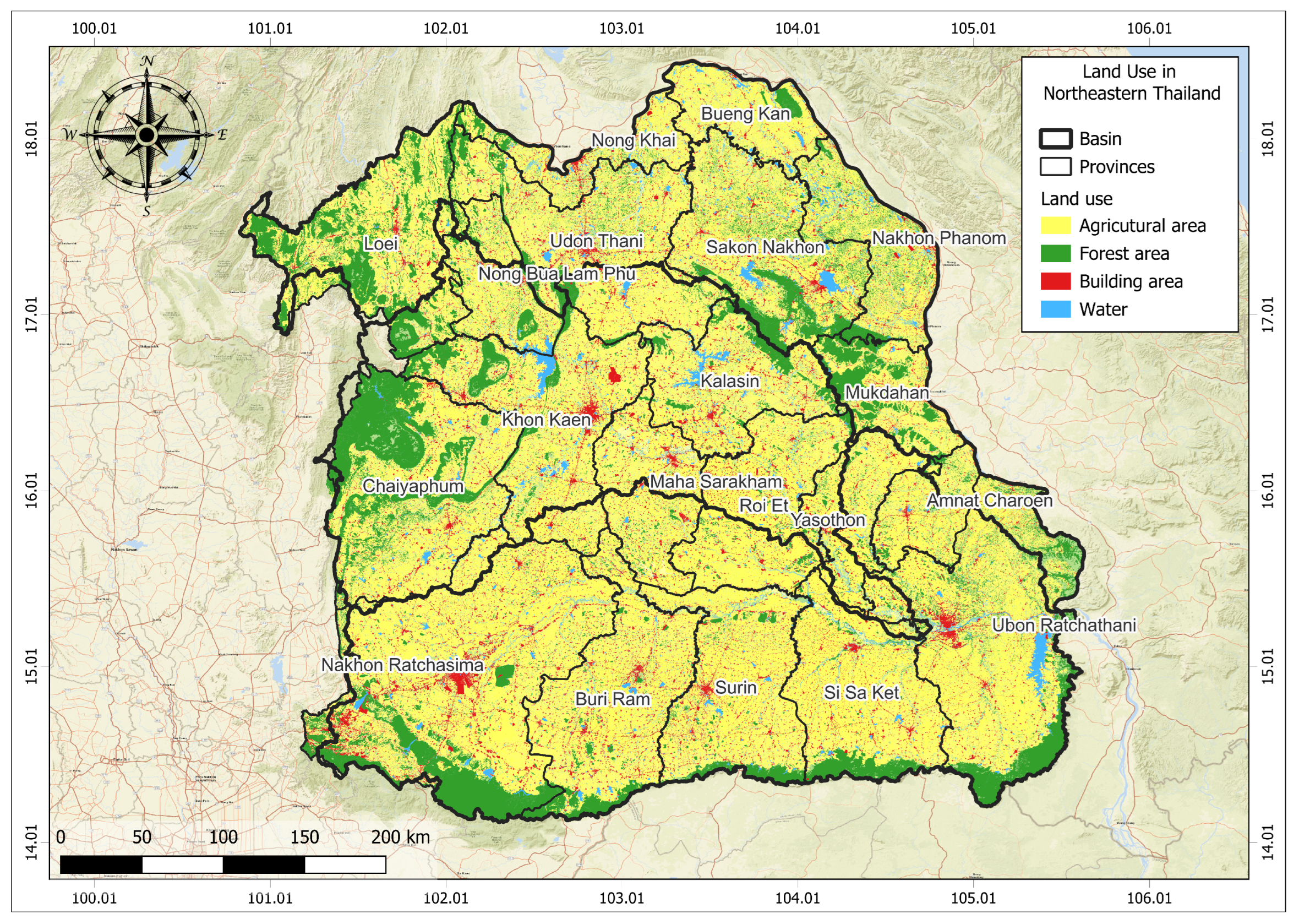
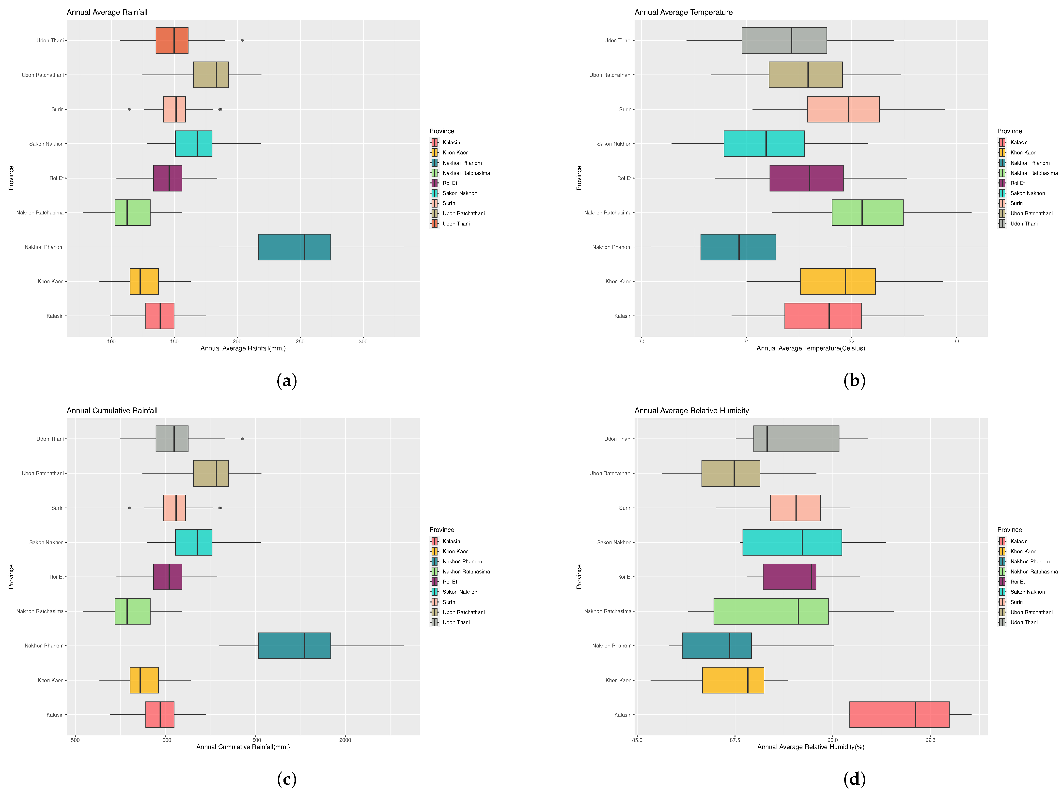
A summary of crop data from the Northeast regions between 1981–2021, including cultivated area (ha), harvested area (ha), productivities (ton), and yield (kg/ha), can be found in the Supplementary Material (Tables S2–S4). Additionally, a comparison between rice productivity and other crop data, encompassing cultivated area (ha), harvested area (ha), and yield per ha (kg) for selected provinces from 1981–2021 is illustrated in Figure 4, Figure 5, Figure 6 and Figure 7.

Rice production and yield in select provinces saw a significant rise from 1981, starting at 13.4 million tons and reaching 38.1 million tons by 2011, marking an impressive growth over a span of 40 years (as depicted in Figure 4, Figure 5, Figure 6 and Figure 7). The initial 20 years witnessed a moderate yearly growth, which nearly doubled post the year 2000. However, post-2011, there has been an observable decline and fluctuation in production. This growth between 1981 to 2011 can be attributed to two factors:

• An expansion in rice cultivation areas, growing from 7.3 million hectares to 12.0 million hectares (a jump of 64%).
• A surge in yield rates, rising from 1.8 tons per hectare to 3.2 tons per hectare. This represents a 78% increase, averaging an annual growth rate of 35.9 kg per hectare.

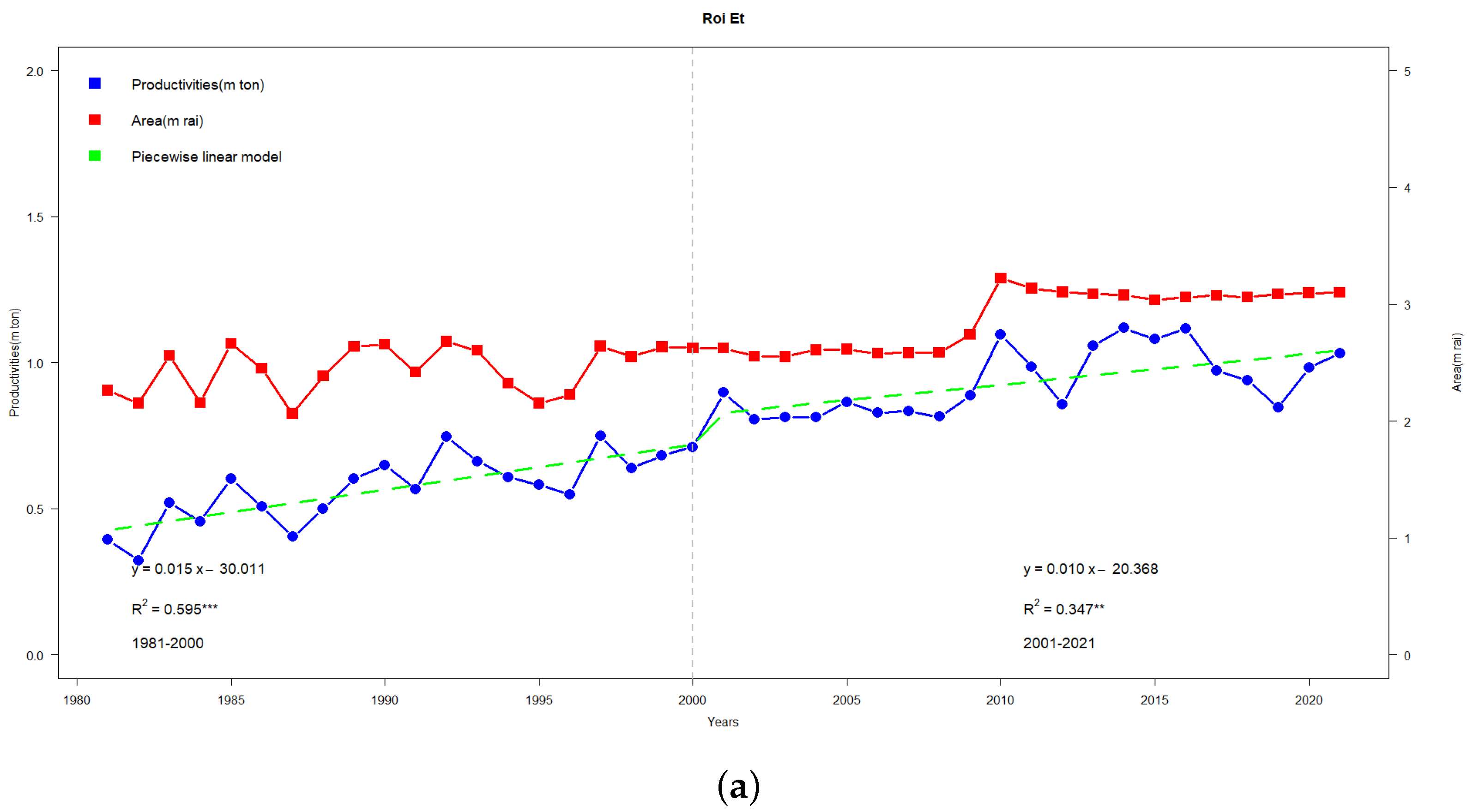
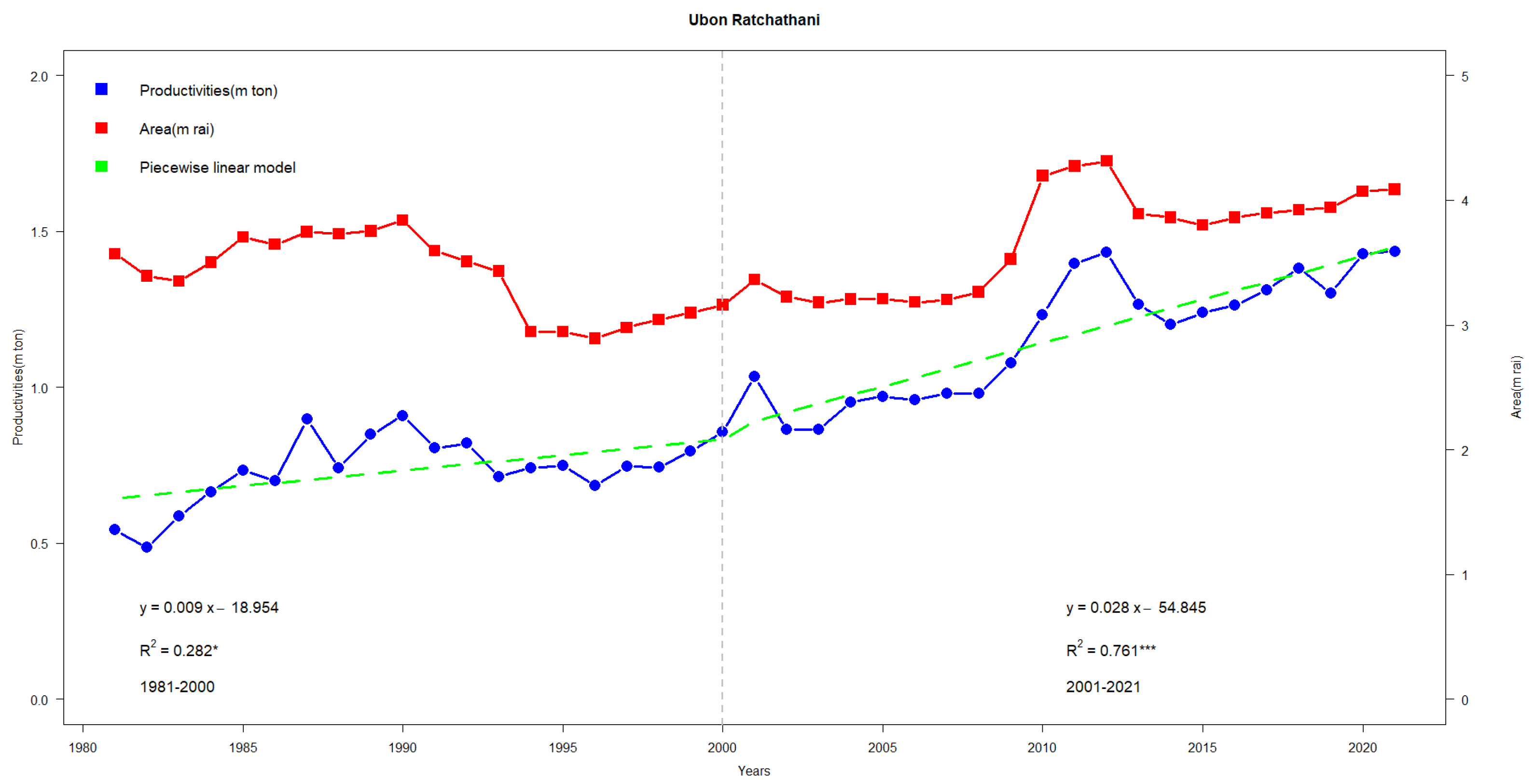
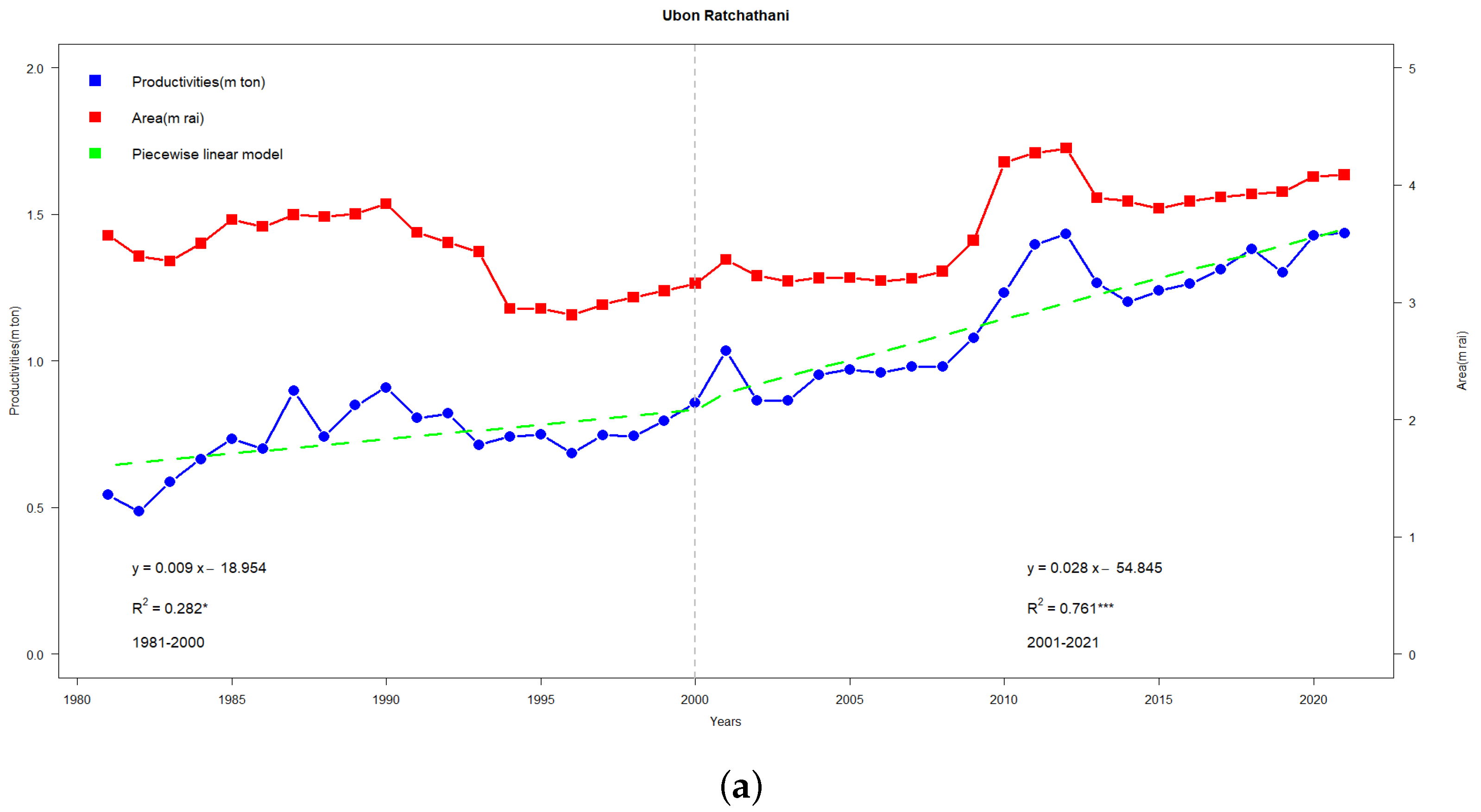
Figure 4a shows highlights on two separate slopes in the production (ton) regression line (blue line)—one from 1981–2000 and the other from 2001–2021, both of which are on an upward trend. For the area (ha), there is a declining slope from 1981–2000, which reverses into an increasing trend from 2001 onwards. These patterns correspond to two regression models: $\widehat{y}=0.009X-18.951$ with $R^2=0.282$ and $\widehat{y}=0.028X-54.845$ with $R^2=0.761$, respectively. From 2000 onwards, there is a noticeable intersection of the production and area regression lines, signaling that an expansion in area is paired with an increase in production.

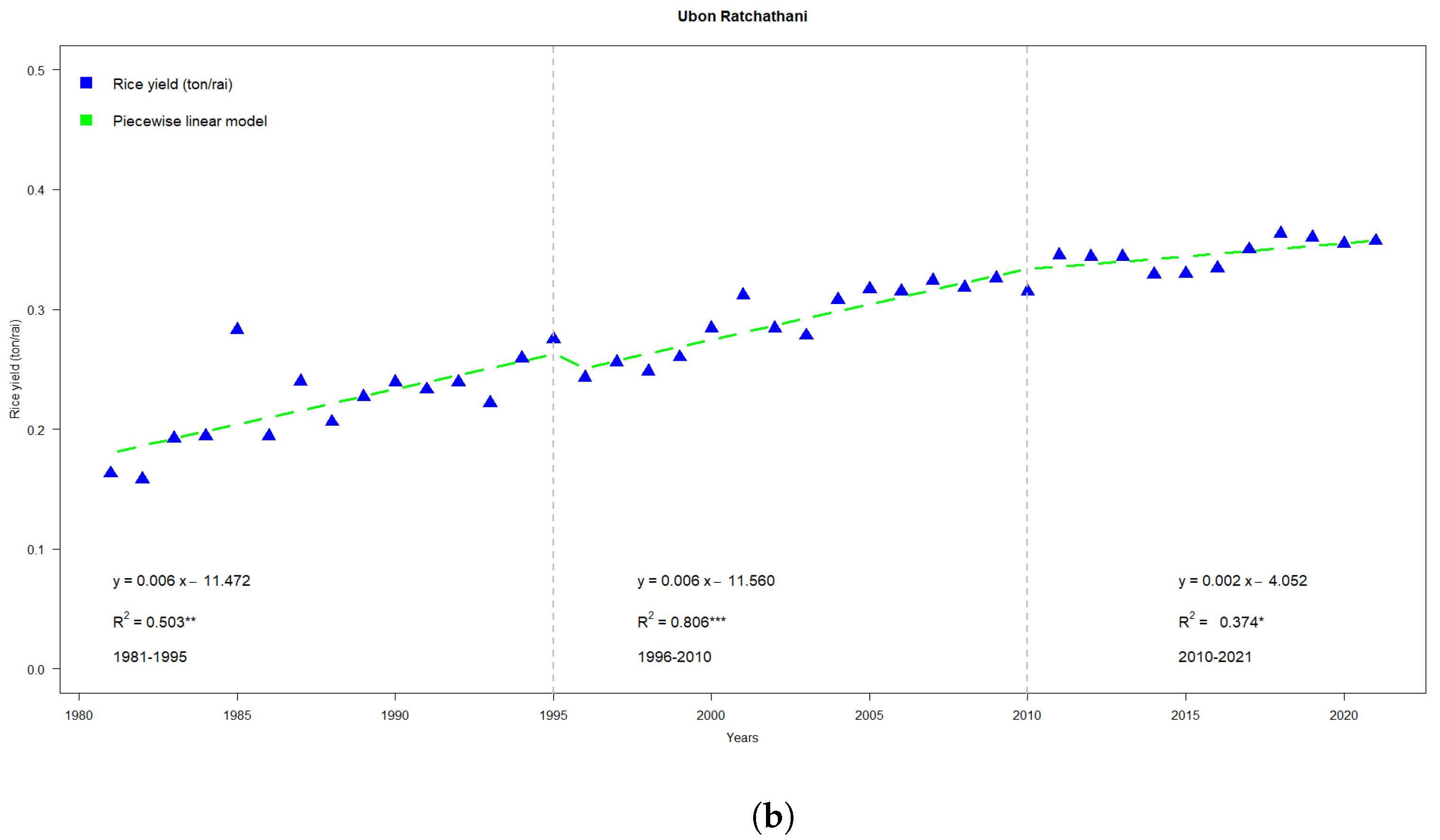
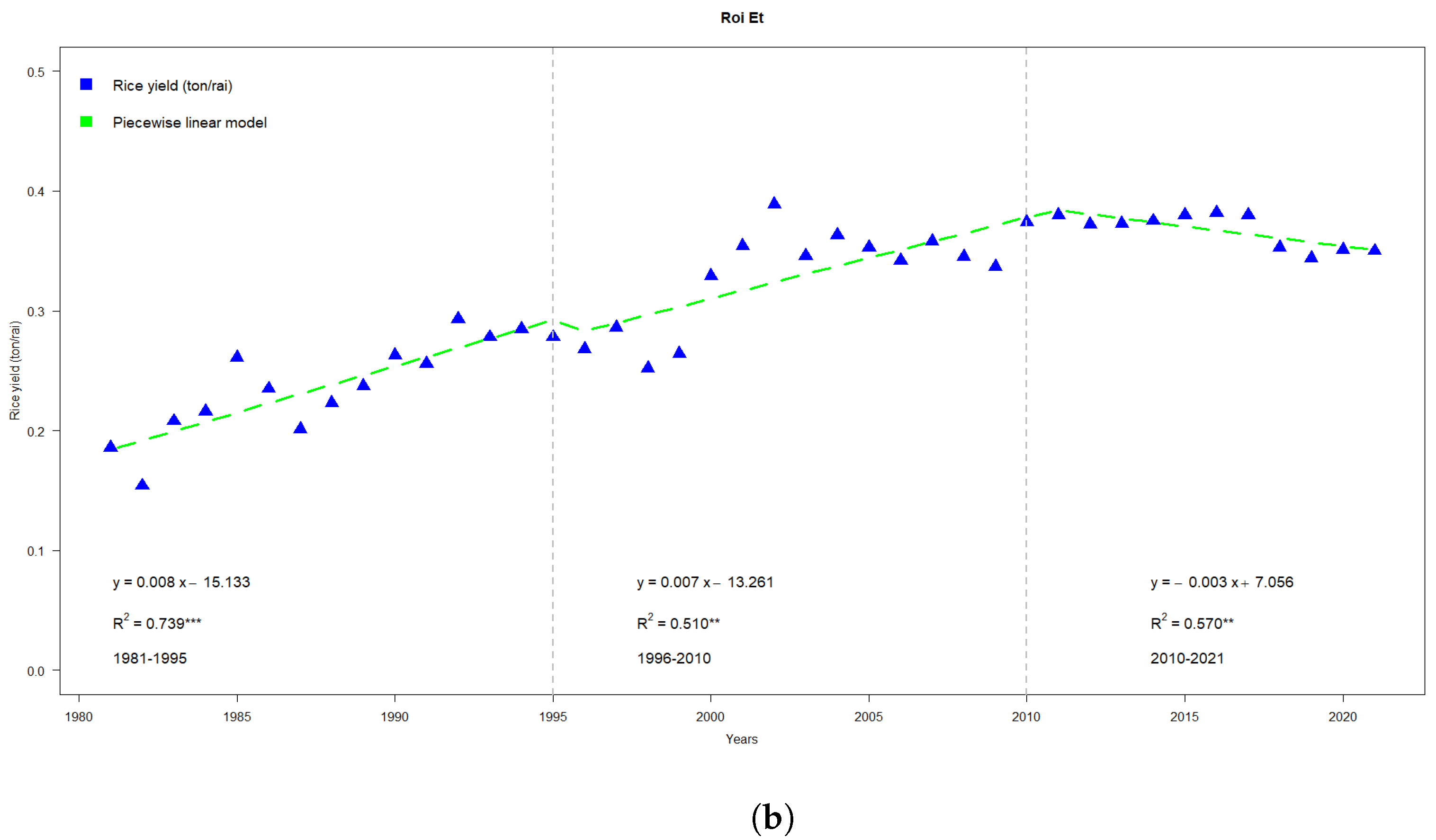
Additionally, Figure 4b shows highlights for three separate slopes in the rice yield (ton/ha)—one from 1981–1995, from 1996–2010, and the other from 2010–2021, all of which are on an upward trend. These patterns correspond to three regression models: $\widehat{y}=0.006x-11.472$ with $R^2=0.503$, $\widehat{y}=0.006x-11.560$ with $R^2=0.806$ and $\widehat{y}=0.002x-4.052$ with $R^2=0.374$, respectively.

Figure 5a illustrates the production (ton) regression line (blue line) with two distinct slopes: a decreasing trend from 1981–2000 and a stable trajectory from 2001–2021. Similarly, the area (ha) showcases a downward slope from 1981–2000, transitioning to a consistent trend from 2001 and beyond. These patterns correspond to two regression models: $\widehat{y}=0.002x+5.201$ with $R^2=0.009$ and $\widehat{y}=0.008X-15.325$ with $R^2=0.461$, respectively.

Additionally, Figure 5b shows highlights for three separate slopes in the rice yield (ton/ha)—one from 1981–1995, from 1996–2010, and the other from 2010–2021, all of which are on an upward trend. These patterns correspond to three regression models: $\widehat{y}=0.01x-2.357$ with $R^2=0.01$, $\widehat{y}=0.003x-4.947$ with $R^2=0.294$ and $\widehat{y}=0.002x+3.451$ with $R^2=0.204$, respectively.

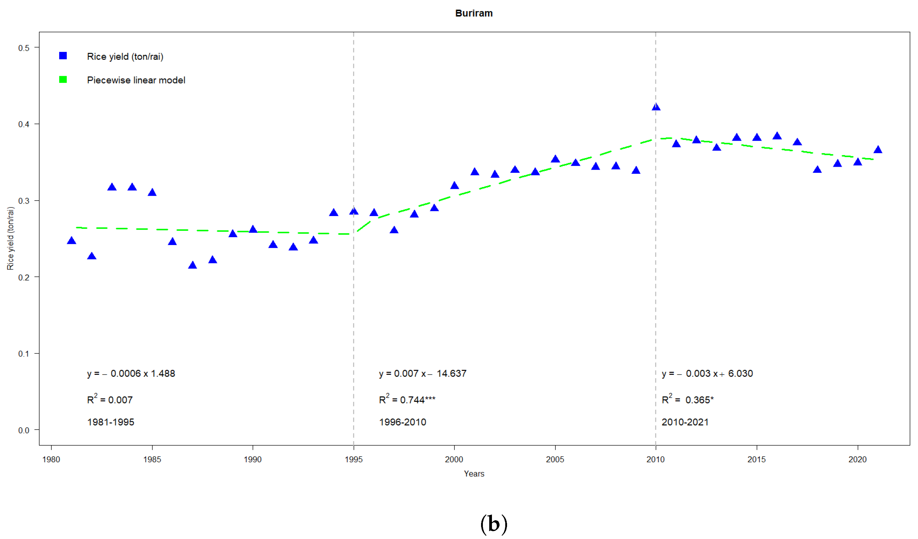
Figure 6a illustrates the production (ton) regression line (blue line) with two distinct slopes: a decreasing trend from 1981–2000 and a decreasing trend with a lower slope from 2001–2021. Similarly, the area (ha) showcases an upward slope from 1981–2000, transitioning to a decreasing trend from 2001 and beyond. These patterns correspond to two regression models: $\widehat{y}=0.015x-30.011$ with $R^2=0.595$ and $\widehat{y}=0.010x-20.368$ with $R^2=0.347$, respectively.

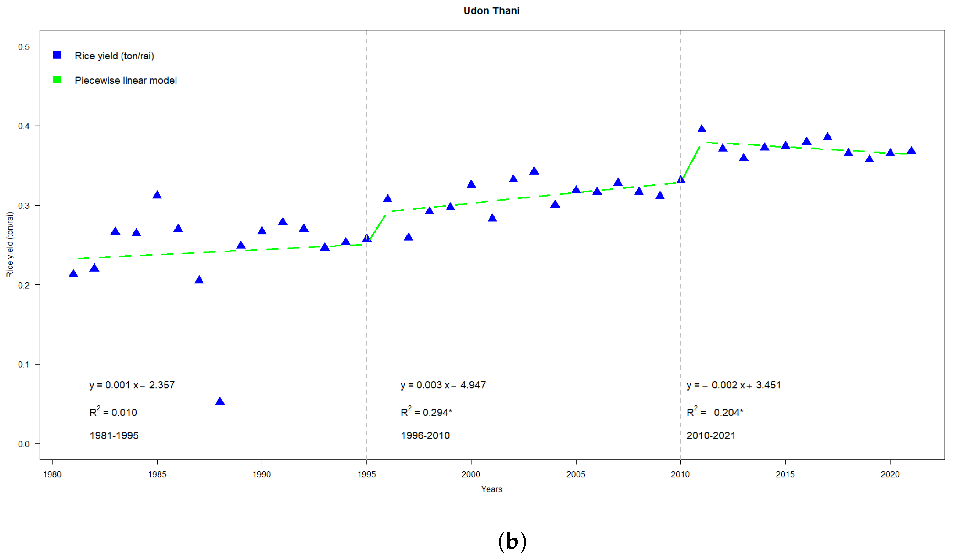
Additionally, Figure 6b shows highlights for three separate slopes in the rice yield (ton/ha)—one from 1981–1995, from 1996–2010, and the other from 2010–2021, two of which are on an upward trend, and the last one is one downward trend. These patterns correspond to three regression models: $\widehat{y}=0.008x-15.133$ with $R^2=0.739$, $\widehat{y}=0.007x-13.261$ with $R^2=0.510$ and $\widehat{y}=0.003x+7.056$ with $R^2=0.570$, respectively.

Figure 7a illustrates the production (ton) regression line (blue line) with two distinct slopes: a decreasing trend from 1981–2000 and a decreasing trend with a lower slope from 2001–2021. Similarly, the area (ha) showcases an upward slope from 1981–2000, transitioning to a decreasing trend from 2001 and beyond. These patterns correspond to two regression models: $\widehat{y}=0.0096x-18.450$ with $R^2=0.173$ and $\widehat{y}=0.004x-7.090$ with $R^2=0.047$, respectively.

Additionally, Figure 7b shows highlights for three separate slopes in the rice yield (ton/ha)—one from 1981–1995, one from 1996–2010, and the other from 2010–2021, two of which are on an upward trend and the last one is on a downward trend. These patterns correspond to three regression models: $\widehat{y}=0.0006x-1.488$ with $R^2=0.007$, $\widehat{y}=0.007x-14.637$ with $R^2=0.744$, and $\widehat{y}=0.003x+6.030$ with $R^2=0.365$, respectively.

In addition, we note that the 1980s were marked by an expansion in rice cultivation areas. This trend plateaued during the 1990s through the early 2000s but then picked up pace rapidly between 2005 and 2011. Unfortunately, post-2011, the cultivated area saw some fluctuations, eventually dipping to 8.7 million hectares by 2016. In terms of yield, the initial decade starting from 1981 experienced a slower growth rate of 20.3 kg per hectare annually, culminating at 1.95 tons per hectare in 1990 (as shown in Figure 4b, Figure 5b, Figure 6b and Figure 7b). The following 21 years up to 2011 marked a rate of increase of 53.5 kg per hectare annually, which translates to a 1.7% yearly surge. However, the subsequent seven years leading up to 2021 did not witness any further rise in yield. The causes behind these shifts in production will be explored in subsequent sections.

3.2. Dependence Analysis

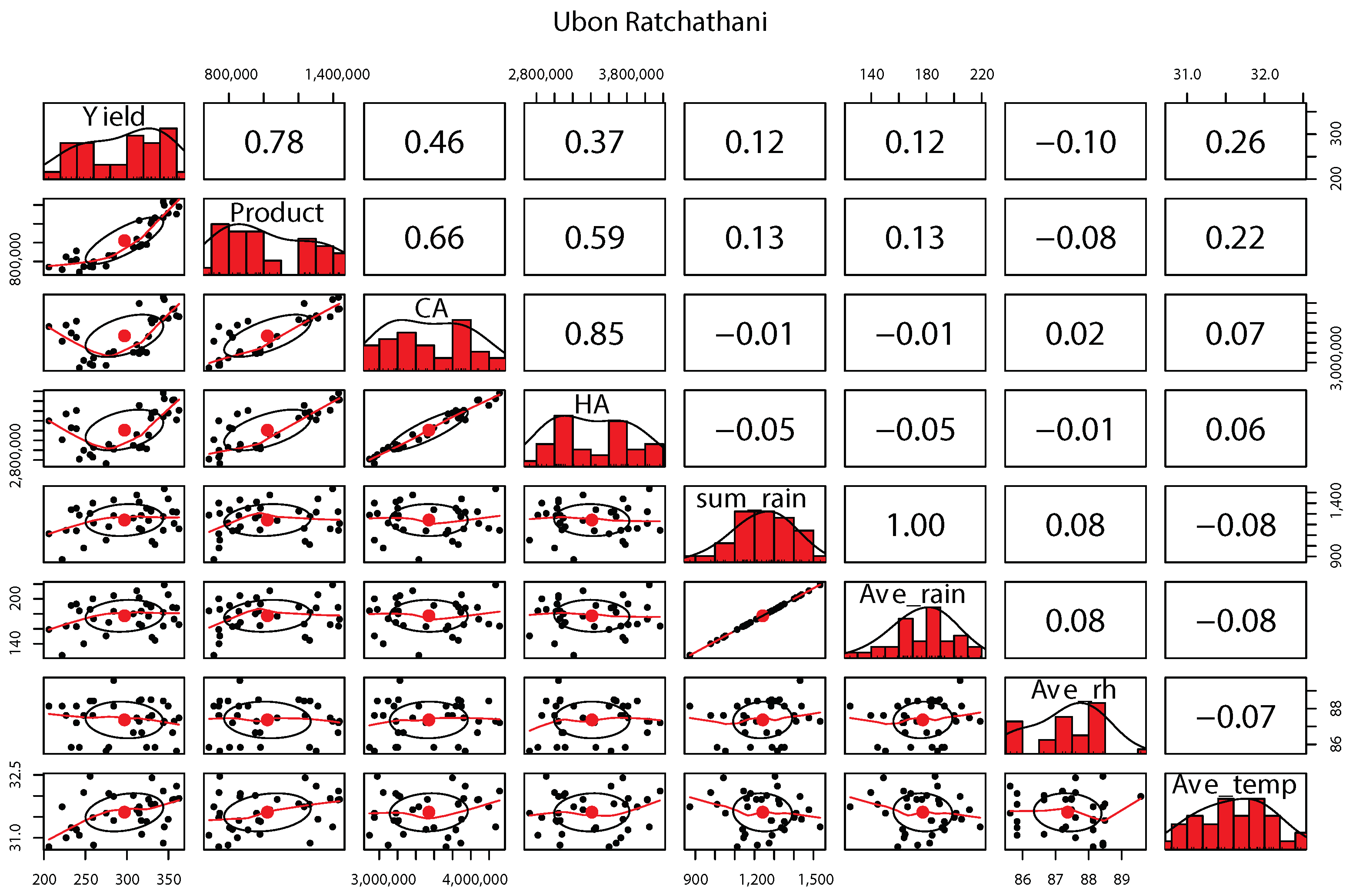
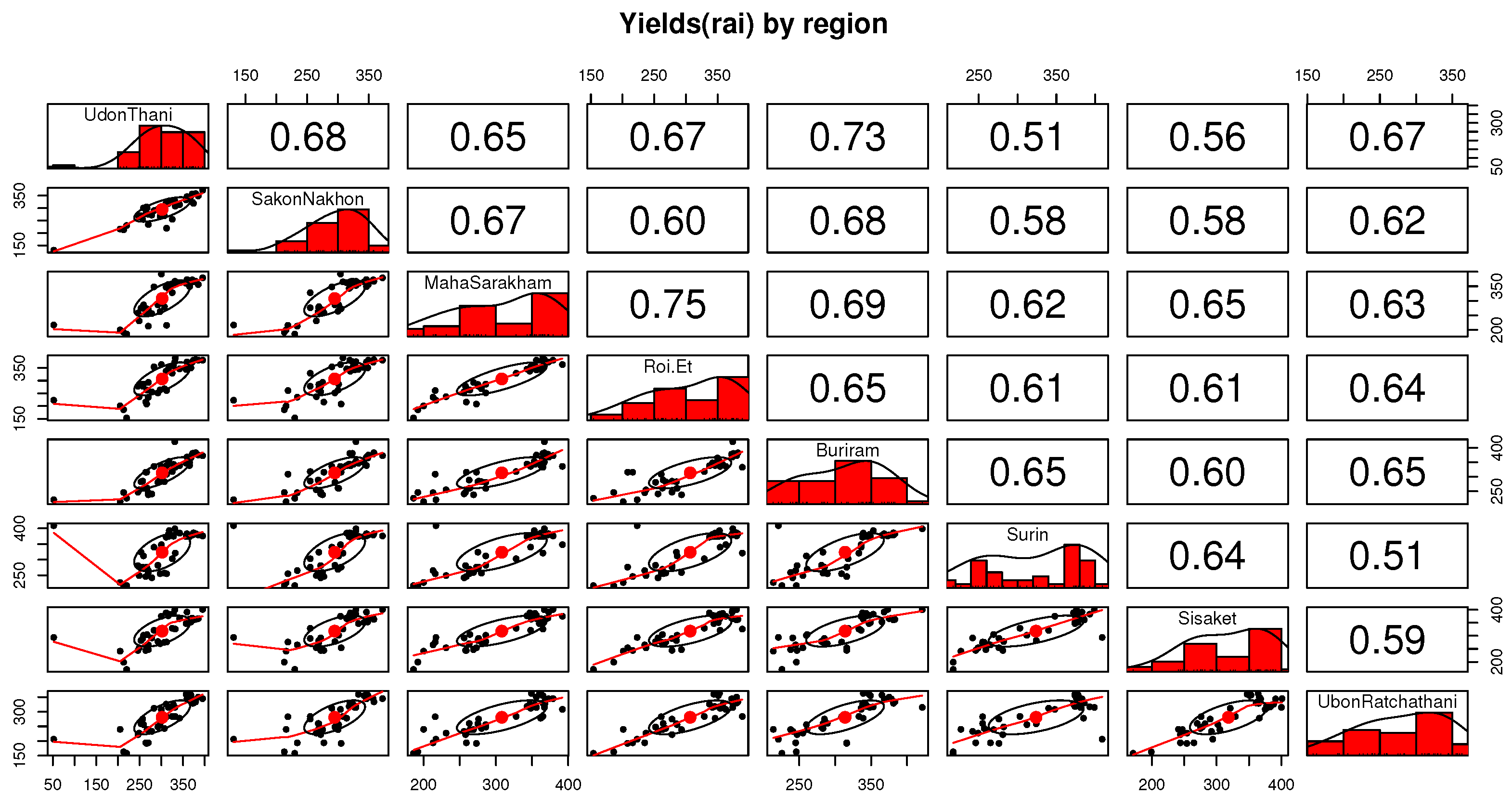
To investigate the interplay between rice production and yield in designated provinces, we utilized seven distinct two-dimensional copula models, as previously described. Figure 8 displays the connection between yields and the selected provinces. In contrast, Figure 9 emphasizes the linkage between crop variables and key meteorological elements.

Figure 8 reveals a strong correlation within agricultural planning for neighboring areas, influenced by water management practices within each watershed. Concurrently, Figure 9 demonstrates the impact or risk assessment of critical meteorological variables, such as cumulative rainfall (mm) and average temperature (°C), on yield (kg) and production (ton).

Results detailing the estimated parameters of the probability distribution for production and yield across various provinces are provided in

Table 4. The estimated parameters of probability distribution for product by each provinces.

Province	Distribution	Estimated Parameters				KS-Test (p-Value)
		Location	Scale	Shape	Rate
Loei	Logistic	768,998.36	-	123,771.70	-	0.06 (0.77)
Nong Bua Lamphu	Logistic	2007.50	-	4.91	-	0.05 (0.79)
Udon Thani	Log-normal	12.42	0.24	-	-	0.13 (0.64)
Nong Khai	Gamma	14.96	-	-	0.001	0.18 (0.57)
Bueng Kan	Normal	144,781.82	11,075.68	-	-	0.02 (0.56)
Sakon Nakhon	Log-normal	13.52	0.31	-	-	0.08 (0.67)
Nakhon Phanom	Gamma	12.35	-	-	-	0.04 (0.64)
Mukdahan	Logistic	525,093.33	97,158.15	-	-	0.09 (0.76)
Amnat Charoen	Log-normal	0.14	12.40	-	-	0.12 (0.65)
Khon Kaen	Weibull	-	445,198.12	4.71	-	0.13 (0.54)
Maha Sarakham	Weibull	-	882,503.07	5.33	-	0.03 (0.54)
Roi Et	Log-normal	12.6159	0.31	-	-	0.08 (0.55)
Kalasin	Normal	2001.50	11.54	-	-	0.06  (0.79)
Yasothon	Log-normal	11.64	0.35	-	-	0.09 (0.63)
Chaiyaphum	Weibull	-	635,372.24	4.90	-	0.11 (0.74)
Nakhon Ratchasima	Log-normal	0.39	12.56	-	-	0.13 (0.51)
Buriram	Normal	864,636.30	226,791.06		-	0.04  (0.84)
Surin	Weibull	-	556,319.22	4.13	-	0.07 (0.77)
Sisaket	Logistic	147,454.04	12,211.24	-	-	0.04 (0.83)
Ubon Ratchathani	Logistic	601,413.29	59,138.35	-	-	0.03 (0.67)

and

Table 5. The estimated parameters of probability distribution for yields by region.

Region	Distribution	Estimated Parameters			KS-Test (p-Value)
		Location	Scale	Shape
UdonThani	Logistic	305.9399	33.9950	-	0.05 (0.47)
SakonNakhon	Weibull	-	313.9020	7.7314	0.05 (0.78)
MahaSarakham	Logistic	312.6092	37.4440	-	0.35 (0.65)
Roi-Et	Weibull	-	332.0968	5.9746	0.26 (0.73)
Buriram	Weibull	-	336.0878	6.9120	0.11 (0.58)
Surin	Logistic	326.8991	37.7011	-	0.36 (0.48)
Sisaket	Weibull	-	342.0744	6.6396	0.18 (0.51)
UbonRatchathani	Weibull	-	304.0702	5.9564	0.12 (0.64)

, categorized based on the main rivers (Khong, Chi, and Mun).

Table 6. The estimated parameters of probability distribution for crop and meteorologic variables for Ubon Ratchathani province.

Region	Distribution	Estimated Parameters			KS-Test (p-Value)
		Location	Scale	Shape
Yield	Weibull	-	316.55	7.84	0.13 (0.54)
Product	Log-normal	13.81	0.24	-	0.15 (0.51)
CA	Normal	1,021,846.29	245,561.08	-	0.15 (0.52)
HA	Log-normal	15.04	0.12	-	0.17 (0.01)
sum_rain	Weibull	-	1305.85	9.70	0.03 (0.84)
Ave_rain	Weibull	-	186.56	9.71	0.03 (0.84)
Ave_rh	Weibull	-	87.85	95.94	0.08 (0.79)
Ave_temp	Normal	31.61	0.45	-	0.05 (0.80)

displays the estimated probability distribution parameters for crop and meteorological variables specific to Ubon Ratchathani province. Each table highlights the fitting distribution and pertinent statistics. In this study, pseudodata based on rank variables are estimated using a copula function, so the estimation of an appropriate peripheral probability distribution is important. Probability distributions such as Weibull distribution, Normal distribution, Log-normal distribution, Gamma distribution, Logistic distribution, and Exponential distribution were considered. The KS test can be used to assess how well each chosen probability distribution fits the data for each province.

Table 4 displays the appropriate distribution of the product for each province, categorized by their respective watersheds: Khong, Chi, and Mun, located in the Northeast. Six distributions, namely Log-normal, Logistic, Gamma, Weibull, and Normal, are identified as suitable for various provinces within the Northeast region. Furthermore, Table 5 presents the fitting distribution of yields for selected provinces. Across all regions, the Logistic and Weibull distributions were found to be the most fitting. Table 6 displays the suitable distribution for both crop and meteorological data specific to the Ubon Ratchathani province.

The subsequent step in our analysis was to validate if the relationships illustrated by the estimated copulas were an accurate reflection of real-world data and whether they were apt for empirical modeling. To evaluate how well the estimated copulas match the empirical data related to rice production and yield, we implemented the described methodology.

One way to gauge the accuracy of copula parameter estimation is to compare the coefficients inferred from the chosen copula with the empirical Kendall coefficients, denoted as $\widehat{\tau }$. We obtained estimates of the Kendall coefficient ($\tau$) for all copulas via a simulation method. These results can be found in

Table 7. The results of the copula function of product between Maha Sarakham and Roi-Et.

Region		$\widehat{\mathit{\tau }}$	Copula	Estimated $\mathit{\theta }$ (s.e.)	S (p-Value)	xv-CIC
Maha Sarakham	Roi-Et	0.77	Normal	0.91 (0.02)	0.04 (0.01)	30.58
			Clayton	2.98 (0.69)	0.12 (0.0005)	10.05
			Frank	15.12 (3.36)	0.02 (0.07)	34.49
			Joe	4.08 (0.86)	0.08 (0.01)	20.41
			Gumbel	3.42 (0.62)	0.003 (0.09)	17.51
			Galambos	2.70 (0.64)	0.003 (0.09)	13.89
			Husler–Reiss	3.20 (0.99)	0.004 (0.09)	10.68

,

Table 8. The results of the optimal copula functions for yields in each regions.

Region		$\widehat{\mathit{\tau }}$	Copula	Estimated $\mathit{\theta }$ (s.e.)	S (p-Value)	xv-CIC
Udon Thani	Sakon Nakhon	0.68	Gumbel	3.17 (0.57)	0.01 (0.05)	28.89
Maha Sarakham	Roi Et	0.75	Frank	12.98 (3.10)	0.02 (0.12)	31.98
Buriram	Surin	0.65	Frank	9.55 (0.92)	0.04 (0.06)	20.70
	Sisaket	0.60	Frank	8.01 (1.85)	0.03 (0.18)	18.37
	UbonRatchathani	0.65	Frank	10.08 (1.62)	0.04 (0.06)	20.76
Surin	Sisaket	0.64	Clayton	3.49 (1.06)	0.03 (0.20)	25.36
	UbonRatchathani	0.59	Clayton	2.83 (1.06)	0.04 (0.18)	19.80
Sisaket	UbonRatchathani	0.51	Clayton	2.07 (0.62)	0.06 (0.03)	12.14

and

Table 9. The results of the copula function between correlated variables at Ubon Ratchathani province.

Variables		$\widehat{\mathit{\tau }}$	Copula	Estimated $\mathit{\theta }$ (s.e.)	S (p-Value)	xv-CIC
Yield	Ave_rain	0.12	Clayton	0.52  (0.39)	0.02 (0.57)	0.35
	Ave_temp	0.26	Clayton	0.97 (0.39)	0.03 (0.40)	3.64
Product	Ave_rain	0.13	Frank	1.16 (1.09 )	0.04 (0.06)	0.04
	Ave_temp	0.22	Gumbel	1.26 (0.16)	0.02 (0.92)	0.78

.

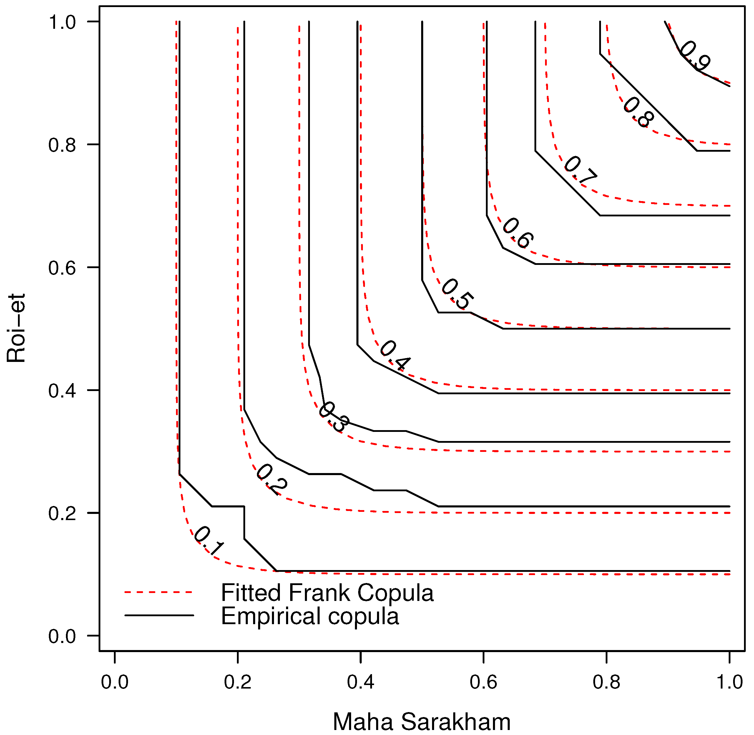
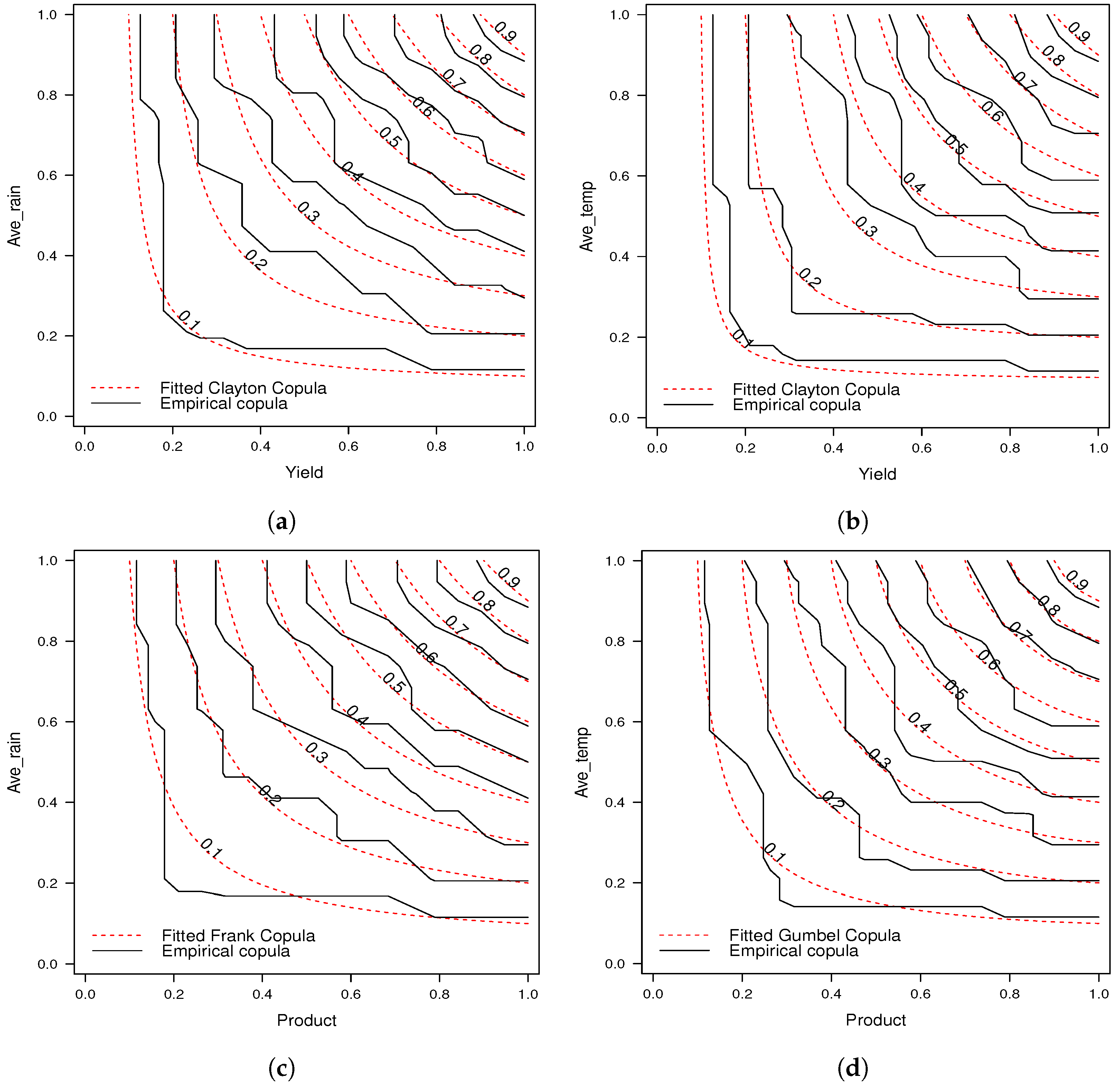
Table 7 presents the outcomes derived from the copula function that examines the product relationship between the Maha Sarakham and Roi-Et provinces. A pronounced correlation is evident, with the Frank copula emerging as the most fitting, having an estimated parameter value of 15.12 and a standard error of 3.36. For enhanced clarity, Figure 10 visually compares the empirical copulas with the fitted copula specific to the Maha Sarakham and Roi-Et provinces, which indicates minimal variance between the empirical and theoretical copula functions.

At the same time, Table 8 presents the Kendall correlation coefficient values, $\widehat{\tau }$, extracted from the sampled data. Every estimated correlation in this table is positive and statistically significant. Among pairs of agricultural products, the combination of Maha Sarakham and Roi-Et provinces displays the most robust correlation with the highest xv-CIC linked to the Frank copula, featuring an estimated parameter of 12.95 and a standard error of 3.10. Conversely, the pair of Srisaket and Ubon Ratchathani exhibits the least substantial correlation associated with the Clayton copula.

Subsequently, Table 9 outlines the results of the copula function relating variables in the Ubon Ratchathani province. The most fitting copula between yield and average rainfall, as well as average temperature, is the Clayton copula. For the correlation between product and average rainfall, the Frank copula is most apt, whereas the Gumbel copula best describes the relationship between product and average temperature.

The findings in Table 8 and Table 9 and Figure 11 corroborate the assessment of how well the copulas fit using the Kendall coefficient $\tau$ and xv-CIC value. For the observation pairs Maha Sarakham and Roi-Et, Burirum and Surin, as well as Sisaket and Ubon Ratchathani, the Frank copula offers the most optimal fit. Conversely, the Clayton copula appears to be the best match for pairs such as Surin and Srisaket and Sisaket and Ubon Ratchathani, while the Gumbel copula is best suited for the Udonthani and Sakon Nakorn pair.

In the case of Ubon Ratchathani province, when examining the relationship between correlated variables, the Clayton copula best represents the link between yield and average rainfall, the Frank copula aptly captures the connection between production and average rainfall, and the Gumbel copula is most fitting for the relationship between production and average temperature.

4. Discussion

Thailand, recognized as a vital player in the global rice market, faces a looming challenge: to sustainably bolster its rice productivity amidst the constraints of environmental and economic adversities. Northeast Thailand, the hub of rice cultivation in the nation, presents a unique case study with its undulating plateau terrain, soil with low fertility, and challenges of saline soil, which are predicted to exacerbate due to climate change [17].

This study aimed to fill the research gap by investigating an optimal copula for the spatial dependence of rice production and related variables in this area. The objective of this study is to understand how rice production in different areas relates to each other in order to improve farming practices and address challenges such as suitable weather. To achieve this goal, we apply three families of copulas—elliptical, Archimedean, and extreme—to analyze crop and meteorological variables across the watershed in the northeastern region of Thailand. Our study identified significant growth in rice production from 1981 to 2011, with variations evident in the specific regions of Udonthani, Roi-Et, Burirum, and others. These patterns have been meticulously represented through regression models that unveil the trends in both cultivated area and yield over the 40-year span. It is not just about recognizing growth patterns. As evident, while Thailand stands tall in rice exports, its yield per hectare lags behind neighbors like Vietnam. Factors, both agronomic and economic—such as soil fertility, climate change impacts, increasing costs of farm chemicals, and labor—are at play [35].

Through the application of two-dimensional copula models, we have explored the intricate spatial dependencies between rice production and yield across various provinces. These models provide an in-depth understanding of how rice productivity in different regions correlates, which is pivotal for formulating region-specific agricultural strategies. Given the challenges confronting Thai farmers, from saline soils to climate-induced droughts, understanding these spatial dependencies is crucial for resilience and sustainability. The distinctiveness in rice production and yield trends across various provinces underscores the regional variations in Thailand’s agricultural landscape.

Maha Sarakham and Roi-Et’s strong dependence contrasts sharply with the relatively weaker correlation observed between Srisaket and Ubon Ratchathani. These variations could be attributed to factors such as local agricultural practices, water resource management, soil fertility, and regional climate conditions. The utilization of different copulas (Frank, Clayton, and Gumbel) to best fit these relationships further accentuates the unique characteristics of each province’s agricultural dynamics. The findings highlight the profound impact of meteorological factors, specifically average rainfall and temperature, on rice production and yield, particularly in Ubon Ratchathani. As climate change continues to influence global weather patterns, understanding these correlations becomes paramount for future agricultural planning and risk management.

Moreover, our data underscore the urgency to adapt to changing climates, especially in regions like Northeast Thailand that are already grappling with saline soils and water scarcity. Global warming’s exacerbation of these challenges emphasizes the need for Thai farmers to innovate and adapt to more water-efficient farming practices. Through our application of elliptical, Archimedean, and extreme copulas, we have tried to solve the research gap, offering a nuanced look into the spatial dependencies of rice production in Northeast Thailand. This understanding is not just academic; it holds profound implications for future agricultural strategies, policy decisions, and on-ground practices to ensure the sustainable progression of Thailand’s rice sector in an ever-evolving global landscape.

5. Conclusions

Thailand’s role as a central player in global agriculture, predominantly in rice cultivation, holds significant implications for both national and global food security. With a projected population increase to 10 billion population by 2050, it becomes increasingly critical to harness innovative techniques that maximize food production, especially in key rice-producing regions like Northeast Thailand. This region, characterized by its unique environmental and climatic challenges, such as saline soils and fluctuating weather patterns, necessitates a dynamic approach to rice cultivation. Our comprehensive study spanning 1981–2021 illuminated nuanced trends in rice production across pivotal provinces in the Northeast. The data reveal a promising trajectory in yields up to 2011, followed by a period of variability, emphasizing the need for adaptive strategies. With the omnipresent challenges of evolving climatic conditions, terrain-specific difficulties, and the looming pressure of escalating production costs, there is a clear mandate for re-imagining agricultural strategies. Utilizing the advanced two-dimensional copula models, our study casts a spotlight on the intricate spatial interdependencies influencing rice yields across the region. This methodology, while invaluable, also highlights the necessity for continual refinement and the adoption of even more sophisticated data analysis techniques in the future.

Conclusively, as Thailand grapples with the dual challenge of sustaining its global market position and addressing its domestic agricultural challenges, the findings from this study provide a pivotal foundation. Emphasizing the importance of region-specific, sustainable agricultural initiatives, the results underscore the value of a more holistic understanding of the factors influencing rice productivity. For future research, it is worth considering the integration of advanced analytical methods, possibly leveraging machine learning or artificial intelligence, to delve even deeper into predicting yield trends and optimizing agricultural practices in the face of changing environmental scenarios.