Abstract
Thousands of debris dangerous to personnel are generated during controlled explosion of warheads containing explosives. To ensure the safety of people, it is necessary to define a zone in which people can stay without risking their lives. A major focus of modern engineering is to maximize the safety of operating technical equipment. In order to implement the above, it is necessary to determine the kinetic energy of the fragments, for which the safe level is below 17 joules (like for air gun). Simultaneous registration of the velocity of such a large amount of fragments is a significant research problem. The article presents a comparison of the two methods of measuring the velocity of splinters formed during detonation of the fragmentation generator. The first common method is to use a chronometer and aluminum foil. The second method, new for this application, is to use a Doppler radar. It allows you to measure the velocity at any moment of the path traveled by the splinter. The article also describes attempts to measure the velocity with both methods, using different variants of Doppler radar settings. Difficulties resulting from the measurements were described, as well as the methods of their elimination.
1. Introduction
The evaluation of the effective range of potential metal fragments generated during work with warheads and explosives is an essential element determining the safety of personnel. The currently applied numerical calculation methods allow for obtaining (by performing numerical simulations) the characteristics of the splitting of the fragments and the distribution of their velocity.
Nowadays, a few different numerical methods are used in the analysis of fragmentation. The authors of the work [1] used different solvers and computer hydrocodes to study the fracture behavior of a 25 mm steel shell. Other scientists [2] investigated the velocity distribution of fragments created by the explosion of a cased charge with two numerical simulation techniques: 2D simulations, 3D simulations using the smoothed-particle hydrodynamic (SPH) method. The numerical simulation of the fragmentation process varying the mechanical characteristics of the shell and type of explosive filling was successfully carried out by the authors of the paper [3]. The SPH method was used by the researchers [4] to investigate numerically the fragmentation process of a cylindrical metal casing. Another research [5] studied the fragmentation calculations of a 120 mm high explosive shell when it was loaded with an advanced HMX-plastic explosive.
Finally, the simulation results should be compared with the real field verification of the quality of fragmentation of the case during stationary tests. However, tests of such type are very costly and time consuming [6,7,8,9,10,11,12,13,14].
In this paper [15], a combined numerical–experimental approach was used to investigate the fragmentation of the warhead. The authors from the Military Institute of Armament Technology (Poland) conducted the experimental tests with the aim of gathering data, which will be useful for the verification of the subsequent simulations. During the experiments after the detonation of the explosive, the fragments of the ruptured shell were collected. The number and the mass distribution of the fragments were examined. Then, numerical simulations were conducted with the same explosive fragmentation geometry as in the experiments. The correctness of the conducted simulations and the applicability of the used numerical technique were verified by comparing the numerical results, especially the fragments’ number and their mass distribution, with the conducted experimental tests’ outcomes. The reasonable agreement between the examined parameters was achieved, which shows that the technique can be used in the future to predict the behavior of fragments [15]. According to the authors’ conclusions, the analysis and comparison of the results obtained from the stationary tests and from the simulation show that the mean total number of fragments created and the number of fragments in the particular mass ranges are very close. The highest differences occur in the number of fragments of the lowest mass range. The differences result from the fact that during stationary tests, it is very hard to recollect such small elements, and that is why the full mass of the casing was not recovered. However, with the increase in fragment mass, the agreement between the simulation results and the experiment rises [15]. The chosen simulations’ results of fragmentation are shown in Figure 1 and Figure 2 and the comparable results of the experimental fragmentation (Figure 3).
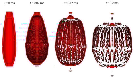
Figure 1.
Example of the analysis of fragmentation of the expanding steel shell [15].
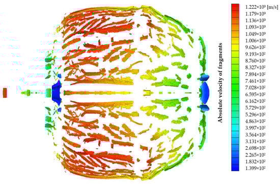
Figure 2.
Velocity distribution of fragments in the simulation [15].
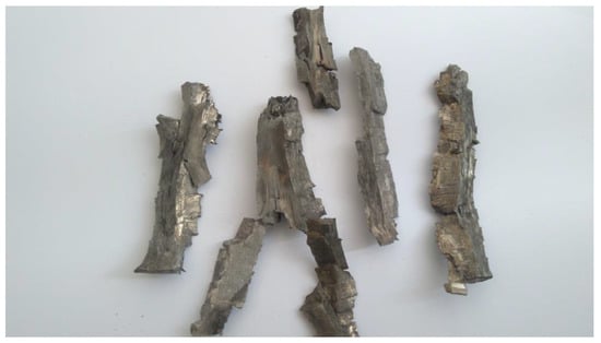
Figure 3.
A few splinters obtained during stationary detonation of the steel shell [15].
With reference to the research results obtained by the authors of the publication [15], the most important aspect is the experimental verification of the velocity of the splinters generated during stationary shell detonation, which at a later stage allows for determining their effective energy, and it compares with simulation results. Obtaining the possibility to compare the velocities of fragments in the experiment and simulations is an important aspect of the verification of the adopted numerical model. In order to be effective, the fragment (splinter) formed as a result of detonation must have appropriate kinetic energy (the kinetic energy of the effective fragment should not be less than 78 joules [16]). For example, fragmentation into large but relatively slow fragments, while also having some advantages, is generally not desirable. Smaller splinters, but in large numbers, are more effective. In addition, they minimize the risk that the targets will be missed [16,17,18,19,20,21]. This article presents a new approach to the problem of recording the velocity of splinters.
2. Materials and Methods
The measurements of the velocity of the fragments were carried out during an experiment of the fragmentation of a stationary steel shell. A 70 mm shell was mounted on a tripod, which was surrounded by large plates—witnesses allocated at various distances. Depending on the needs, they were made of plywood, steel, or aluminum. A replacement fuse was screwed into the shell and detonated remotely. During the fragmentation of the shell, a cloud of debris spread around, striking the witness plates. Individual impacts and punctures can be observed on the plates. The plates usually stick to each other to form a full circle around the fragmented projectile. Traces on the plates made it possible to estimate the size of the fragments, their number, propagation, and arrangement per square meter. By adjusting the distance of the plates from the projectile and changing their thickness, it was possible to estimate the effective radius of destruction of the fragments in a practical way. However, in this case, several fragmentations had to be carried out, which was associated with a high cost of research. Alternatively, a circle of plates can be divided into several parts, and each part can be placed at a different distance from the fragmented projectile. From the scientific and research point of view, determining the velocity of the fragments with their known mass would allow determination of the kinetic energy. To measure the velocity of standard objects, such as projectiles, the most commonly used are appropriate induction gates, optical gates, or a Doppler radar. However, there are difficulties in measuring the velocity of the fragments that are not present in the case of measuring the velocity of the projectile. When measuring the velocity of the projectile, the direction of the flight path is well known. Moreover, the projectile is the only object that moves during the measurement. In the case of a series of projectiles, the time difference between the individual shots is long enough for undisturbed measurement.
In the case of determining the velocity of the fragments, the process becomes more complicated. The debris spreads out simultaneously in different directions. It is impossible to use gates or a Doppler radar directly close to the fragmented shell. The equipment would be damaged by the detonation wave and debris.
Until now, the velocity of fragments was measured using a chronometer and aluminum foils. It is based on delivering two signals to the chronometer: starting and stopping time measurement. The moment of detonation of the shell is the start of the measurement of time, and the moment the fragment hits the plate, the measurement of time is stopped. Knowing additionally the distance from the shell to the plate, it is possible to calculate the average velocity of the fragment on the flight path.
The measurement is started by two leads attached to the head and connected to a chronometer. They are isolated from each other. Upon detonation, the high temperature melts the insulation between them, causing an electrical short circuit. The chronometer interprets this as a signal to start the measurement. The individual boards are covered with aluminum foils, insulated from the steel board with a laminate. One wire is connected to the steel plate, and the other wire to the aluminum foil. When the aluminum foil, laminate, and board are punctured by a splinter, the foil is shorted with the board, and the circuit is closed, and the timer interprets it as a signal to stop the time measurement. An illustrative diagram is shown in Figure 4.
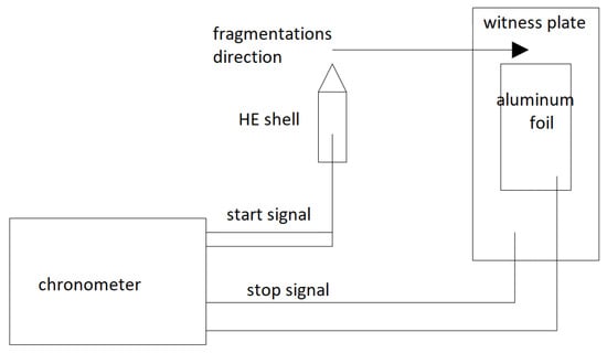
Figure 4.
Diagram of the station for measuring the velocity of the splinters with the contact method.
The method described above is quite simple but considerably inaccurate. Generally, after fragmentation, the plates are covered with splinters’ holes, and it is impossible to estimate which splinter stopped the time measurement. The aluminum foil method does not solve this basic problem and only allows for calculating the average velocity of the splinter. In conclusion, the method with aluminum foils is not accurate enough.
Taking the above into account, the authors decided to use Doppler radar technology for the velocity measurement of the splinters. Two Weibel’s Doppler radars were used during the tests. The first radar (SL-528PE) was located in the bunker about 4 m from the fragmented shell. It was directed towards the most distant plate. The second radar (SL-520P) was placed in the bunker behind the plate. It was directed with a mirror towards the fragmented shell through a small window in the plate (Figure 5).
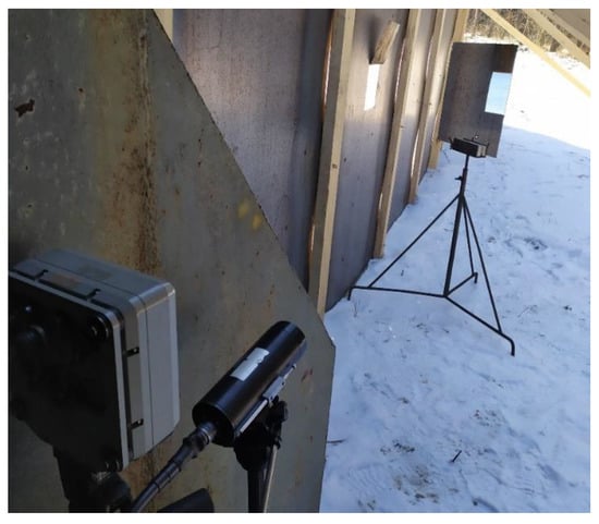
Figure 5.
The Doppler radar with the mirror.
The radar could not be allocated directly at the detonating object because of the possibility of damage of the equipment. The window in the plate reduced this possibility to the minimum. The configuration scheme is shown in Figure 6.
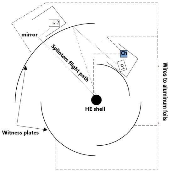
Figure 6.
The configuration of the Doppler radars. Ch—chronometer; R—Doppler radar.
3. Results
During the stationary detonation test, the 70 mm steel shell was used. The shell was surrounded by four quarter circles made of steel plates with four different radii: 5, 9, 14, 21 m. On each quarter circle, one aluminum foil was stuck and connected to the chronometer. The shell filled by the explosive was detonated by using a blaster and a replacement fuse (Figure 7).
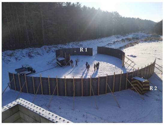
Figure 7.
The configuration of the fragmentation test stand.
After the detonation, the measurement results were recorded and then analyzed. Both radars recorded the velocities of the splinters. Radar 2 emitted the radiation through the mirror and was able to record the fragment, which moved in a straight line, and registered the velocity of the splinters (directly from the radar point of view). Radar 1, observing the plate from the inside, recorded much more debris, which distorted the velocity chart. Due to its hardware limitation, the chronometer only measured time in three quarter circles.
The velocity versus time graphs (Figure 8, Figure 9, Figure 10 and Figure 11) and the corresponding data in the tables (Table 1 and Table 2) are shown below for the chosen detonation, additionally comparing radars 1 and 2.
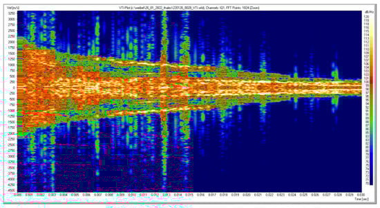
Figure 8.
The screen of the graph of radial velocity versus time of all recorded fragments (radar 1). Left vertical axis—radial velocity (m/s); right vertical axis—signal frequency (dB, Hz); horizontal axis—time (s).
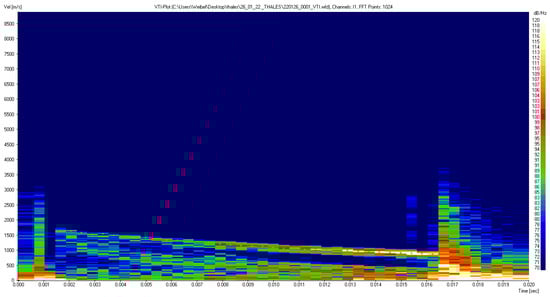
Figure 9.
The screen of the graph of radial velocity versus time of all recorded fragments (radar 2). Left vertical axis—radial velocity (m/s); right vertical axis—signal frequency (dB, Hz); horizontal axis—time (s).
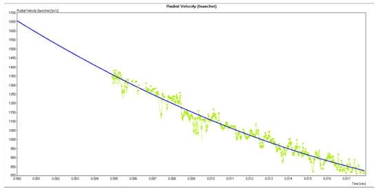
Figure 10.
The graph of the radial velocity versus time of a separated single splinter (radar 1). Left vertical axis—radial velocity (m/s); horizontal axis—time (s).
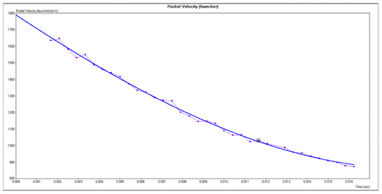
Figure 11.
The graph of the radial velocity versus time of a separated single splinter (radar 2). Left vertical axis—radial velocity (m/s); horizontal axis—time (s).

Table 1.
Recorded data for a separated single splinter (radar 1).
Table 2.
Recorded data for a separated single splinter (radar 2).
In order to compare the measurements made with the chronometer (Figure 12) and the radar, the average velocities of the individual flight sections were calculated. The comparison results for the chosen splinter are presented below (Table 3).
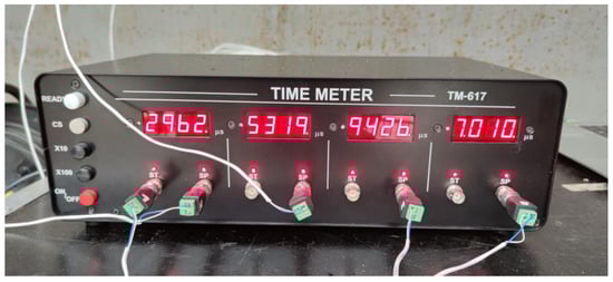
Figure 12.
Laboratory chronometer TM-617 with the recorded flight time of debris.
Table 3.
The chronometer and the radar average velocities.
4. Discussion
The images recorded by radars 1 and 2 (Figure 8 and Figure 9) show comparatively the distribution of the recorded flight paths of the splinters depending on the width of the recording field.
Significantly, the negative values of the fragment velocity are observed on radar 1. The cause of the signal in the negative velocities, also known as the image spurious signal, is the finite image rejection in the downconverting mixer. Depending on the model of Weibel’s radar, it will have different requirements for the suppression of this image signal, but in all cases, it is suppressed enough for the processing software to identify it as a spurious signal and not create a false track for it. For velocity radars and their fairly simple measurement scenarios, the requirements for the image suppression are quite low (>20 dB compared with the real signal). For larger instrumentation radar systems (like radar 1), the typical performance is in excess of 30 dB, which is more important in these cases as they support scenarios more likely to have many targets occurring at once—some of which might have opposite velocities potentially overlapping with image spurious signals, which might degrade their signal-to-noise ratio and detection probability.
The results recorded by radar 2, thanks to the application of the limited field of view (through the window cut out in the cover), more accurately express the flight paths of the selected fragments. These differences are visible in the comparison of Figure 10 and Figure 11. In the case of the velocity recording signal of the selected fragment from radar 1 (Figure 10), a significant dispersion of the values of the measurement points can be seen on the basis of which the radar software traced the trend line of the fragment’s velocity versus time.
The signal for recording the velocity of the selected fragment from radar 2 (Figure 11) contains the values of the measuring points with a small dispersion in relation to the plotted trend line of the fragment’s velocity versus time. On the basis of the obtained results, it can be concluded that the measurement configuration with radar 1 can be used for the general assessment of the propagation of fragments in the selected angular zone limited by the concave surface of the witness’s plate signal reflection, while the station with radar 2 can be used for the selective measurement of fragments whose velocity is determined continuously, and enabling them to be captured (after using an bullet trap) will allow for determining their kinetic energy.
Regarding the averaged values of the velocity of the splinter (Table 3) for the various measurement methods, it can be concluded that the results are comparable for both 5 and 14 m distances. It should be taken into account that the aluminum foil and the radar most probably measured the velocity of two different fragments (with the differences no more than 1%). Additionally, the differences may be generated during the moment of the start of the measurement time. For the Doppler radar, the moment of starting the measurement is the flash at the moment of detonation. For the chronometer, the measurement starts after the insulation is melted down (which occurs later than the flash). The questionable result of the average velocity calculated by the chronometer for the 9 m distance may be related to the fact of premature electrical short circuit between the foil and the plate.
5. Conclusions and Advice
Doppler radar measurement is a more accurate method compared with the contact method. It allows the measurement of the splinters’ velocity along the entire flight path. In order to reduce the interference caused by other debris, the window in the plate can be reduced proportionally. An interesting solution would be to place the tube from the head to the hole with the mirror. Doppler waves would affect only the objects in the tube, which should improve the quality of velocity recording. Importantly, the radar measurement will allow for experimentally measuring the kinetic energy of the fragment. A bullet trap placed behind the mirror would catch the fragment, which can then be weighed. It is important for the estimation of the kinetic energy and the precise determination of the effective radius of splinters. However, the most important achievement, according to obtained results of experimental research, is the possibility to compare them with the results of numerical simulations. Of course, other noncontact measurement methods can be used for speed measurements, such as the laser method, photonic Doppler method, and high-speed photography; however, this requires many comparative tests with the currently used method to determine the accuracy of measurements and the possibility of protecting measuring devices against splinters.
On the basis of the obtained results, it is possible to refine the numerical model of the fragmentation process so that it can be used to determine safety zones with the required accuracy.
Author Contributions
Conceptualization, A.W. and M.M.; methodology, A.W.; software, A.W.; validation, P.S.; formal analysis, A.W.; investigation, P.S.; resources, M.M.; data curation, A.W.; writing—original draft preparation, M.M.; writing—review and editing, M.M.; visualization, A.W.; supervision, P.S.; project administration, A.W.; funding acquisition, P.S. All authors have read and agreed to the published version of the manuscript.
Funding
This research received no external funding.
Institutional Review Board Statement
Not applicable.
Informed Consent Statement
Not applicable.
Data Availability Statement
Not applicable.
Conflicts of Interest
The authors declare no conflict of interest.
References
- Moxnes, J.F. Experimental and numerical study of the fragmentation of expanding warhead casings by using different numerical codes and solution techniques. Def. Technol. 2014, 10, 161–176. [Google Scholar] [CrossRef]
- Grisaro, H.; Dancygier, A. Numerical study of velocity distribution of fragments caused by explosion of a cylindrical cased chargé. Int. J. Impact Eng. 2015, 86, 1–12. [Google Scholar] [CrossRef]
- Ugrcic, M. Numerical Simulation of the Fragmentation Process of High Explosive Projectiles. Sci. Tech. Rev. 2013, 63, 47–57. [Google Scholar]
- Xiangshao, K.; Weiguo, W.; Jun, L.; Fang, L.; Pan, C.; Ying, L. A numerical investigation on explosive fragmentation of metal casing using Smoothed Particle Hydrodynamic method. Mater. Des. 2013, 51, 729–741. [Google Scholar]
- Elshenawy, T.; Zaky, M.G.; Elbeih, A. Experimental and numerical studies of fragmentation shells filled with advanced HMX-plastic explosive compared to various explosive charges. Braz. J. Chem. Eng. 2022, 1–12. [Google Scholar] [CrossRef]
- Richard, M. Lloyd, Conventional Warhead Systems Physics and Engineering Design; AIAA: Reston, VA, USA, 1998; pp. 21–53. [Google Scholar]
- Junpeng, C.; Zaiqing, X.; Qiang, M.; Tian, G. Engineering calculation method on the relation between the velocity of built-in warhead fragments and shell. J. Ordnance Equip. Eng. 2018, 39, 12–15. [Google Scholar]
- Karpenko, A.; Ceh, M. Experimental simulation of fragmentation effects of an improvised explosive device. In Proceedings of the 23rd International Symposium on Ballistics, Tarragona, Spain, 16–20 April 2007; pp. 16–20. [Google Scholar]
- Held, M. Fragment mass distribution of HE projectiles. Propellants Explos. Pyrotech. 1990, 15, 254–260. [Google Scholar] [CrossRef]
- Arnold, W.; Rottenkolber, E. Fragment mass distribution of metal cased explosive charges. Int. J. Impact Eng. 2008, 35, 1393–1398. [Google Scholar] [CrossRef]
- Zhang, Z.; Huang, F.; Cao, Y.; Yan, C. A fragments mass distribution scaling relations for fragmenting shells with variable thickness subjected to internal explosive loading. Int. J. Impact Eng. 2018, 120, 79–94. [Google Scholar] [CrossRef]
- Wittel, F.K.; Kun, F.; Herrmann, H.J.; Kröplin, B.H. Fragmentation of Shells. Phys. Rev. Lett. 2004, 93, 035504. [Google Scholar] [CrossRef] [PubMed]
- Wittel, F.K.; Kun, F.; Herrmann, H.J.; Kröplin, B.H. Breakup of shells under explosion and impact. Phys. Rev. 2005, E 71, 016108. [Google Scholar] [CrossRef]
- Hernandez, G.; Herrmann, H.J. Discrete models for two- and three-dimensional fragmentation. Physica A 1995, 215, 420. [Google Scholar] [CrossRef]
- Gorska, A.; Zochowski, P.; Zielenkiewicz, M. Experimental and Numerical Study of the Fragmentation of Warhead Casings. In Proceedings of the 30th International Symposium on Ballistics, Long Beach, CA, USA, 11–15 September 2017; pp. 1622–1628, ISBN 978-1-60595-419-6. [Google Scholar]
- Wu, C.; He, Q.-G.; Chen, X.; Zhang, C.; Shen, Z. Debris cloud structure and hazardous fragments distribution under hypervelocity yaw impact. Def. Technol. 2022, in press. [Google Scholar] [CrossRef]
- Piątek, B.; Zarzycki, B. Simulators of fragments. Probl. Tech. Uzbroj. 2016, 138, 87–97. [Google Scholar]
- Zarzycki, B. Analysis of selected methods of forced fragmentation of artillery shells. Probl. Tech. Uzbroj. 2016, 138, 25–34. [Google Scholar]
- Długołęcki, A.; Dębiński, J.; Faryński, A.; Kwaśniak, T.; Słonkiewicz, Ł.; Ziółkowski, Z. Measurements of characteristics for fragmentation bursting heads. Probl. Tech. Uzbroj. 2021, 157, 59–79. [Google Scholar]
- Kwiecień, C. A concept of the air drag law for spherical fragments prepared on the basis of AASTP-1 allied publication data. Probl. Tech. Uzbroj. 2018, 146, 73–91. [Google Scholar] [CrossRef]
- Guzek, E. Problematyka wyznaczania stref ochronnych wokół magazynów oraz składów materiałów i przedmiotów wybuchowych. Probl. Tech. Uzbroj. 2013, 126, 21–40. (In Polish) [Google Scholar]
Disclaimer/Publisher’s Note: The statements, opinions and data contained in all publications are solely those of the individual author(s) and contributor(s) and not of MDPI and/or the editor(s). MDPI and/or the editor(s) disclaim responsibility for any injury to people or property resulting from any ideas, methods, instructions or products referred to in the content. |
© 2023 by the authors. Licensee MDPI, Basel, Switzerland. This article is an open access article distributed under the terms and conditions of the Creative Commons Attribution (CC BY) license (https://creativecommons.org/licenses/by/4.0/).