Abstract
In order to achieve rapid and fair distribution of emergency supplies after a large-scale sudden disaster, this paper constructs a comprehensive time perception satisfaction function and a comprehensive material loss pain function to portray the perceived satisfaction of disaster victims based on objective constraints such as limited transport, multimodal transport and supply being less than demand, and at the same time considers the subjective perception of time and material quantity of disaster victims under limited rational conditions, and constructs a multi-objective optimisation model for the dispatch of multi-cycle emergency supplies by combining comprehensive rescue cost information. For the characteristics of the proposed model, based on the NSGA-II algorithm, generalized reverse learning strategy, coding repair strategy, improved adaptive crossover, variation strategy, and elite retention strategy are introduced. Based on this, we use the real data of the 2008 Wenchuan earthquake combined with simulated data to design corresponding cases for validation and comparison with the basic NSGA-II algorithm, SPEA-II and MOPSO algorithms. The results show that the proposed model and algorithm can effectively solve the large-scale post-disaster emergency resource allocation problem, and the improved NSGA- II algorithm has better performance.
1. Introduction
In recent years, earthquakes, droughts, floods and other natural disasters have occurred frequently, bringing huge casualties and economic losses to human society, with earthquakes posing a serious threat to people’s lives and property with their suddenness and destructiveness. After an earthquake, the emergency relief system in the affected area must respond quickly to minimise the various types of damage caused by the disaster, and the distribution and transport of emergency supplies after the disaster becomes a prerequisite for the smooth implementation of post-disaster emergency relief. In view of the relative scarcity of emergency supplies in post-disaster situations, the rational and effective selection of transport solutions for the distribution of supplies is essential to increase the satisfaction of the affected population and enhancing the overall relief effect. Therefore, how to effectively mobilise the emergency logistics distribution system after a disaster and distribute supplies to the victims in a fair and timely manner has become the focus of research by scholars in various countries, and this is also the main research content of this paper.
The remainder of the paper is organised as follows. Section 2 presents an overview of the relevant literature. Section 3 describes the specific problem under study, and the process of constructing the objective function. Section 4 presents the emergency material distribution and transportation model. Section 5 presents the algorithm used to solve the problem, and the process of algorithm improvement. In Section 6, we conduct experiments and analysis for a specific case to verify the scientificity, feasibility and superiority of the model and algorithm in this paper. Finally, Section 7 concludes the paper.
2. Literature Review
Domestic and international scholars have studied the emergency rescue process from different perspectives. Early research on the distribution and transportation of emergency supplies focused on improving the efficiency of rescue, Knott R [1] developed a single linear programming model to study the transportation of bulk food from a single relief point to multiple disaster sites, with the objective of minimizing the cost of delivering supplies and maximizing the amount of supplies available to the victims in the emergency response system. Ray [2] considered post-disaster transport capacity constraints and established a multi-cycle emergency material deployment model for a single material, with the objective of minimising transport costs and out-of-stock costs. Haghani et al. [3,4] established a multi-cycle, multi-material network flow model and solved the efficiency problem in emergency material distribution by minimizing emergency material transportation costs. Barbarosoglu et al. [5] established a two-stage emergency material dispatch model with the objective of minimizing rescue time and total rescue cost to study the timely dispatch of emergency rescue materials. Ma et al. [6] considered multimodal transport according to the characteristics of multi-stage post-disaster relief, and established a multi-stage dynamic multimodal transport model for emergency materials based on the mixed integer planning method, and solved the problem of transporting emergency materials under disaster conditions by minimizing the most transport costs. Zhu et al. [7] addressed the problem of dispatching emergency medical supplies under sudden disaster events; they considered the limited nature of emergency medical supplies after disasters from the perspective of minimizing the unmet demand and total supply delay time in the disaster area, and used a local search algorithm with the introduction of a stochastic search strategy to solve the problem. Liu et al. [8] studied the problem of dispatching emergency supplies at multiple dispatch points under demand constraints according to the characteristics of continuous consumption of emergency supplies, and they established emergency models with the minimum number of dispatch points under the earliest emergency time premise and the minimum number of dispatch points under the restricted period condition respectively, both of which achieved better optimisation results. From the above studies, early research focused on maximising the efficiency of emergency relief in the process of dispatching emergency resources, specifically in terms of minimising the total cost of relief [9], minimising the total relief time [10,11] and maximising the rate of material satisfaction of the affected people as the decision-making objectives. The above research has enriched the emergency logistics system and laid the foundation for the timely supply and decision making of emergency supplies after a disaster.
However, in a large-scale disaster, the delivery of supplies to the affected areas for reasons of efficiency alone does not achieve a satisfactory result for the affected population. People in the affected areas are facing huge losses and trauma and are very sensitive to the emergency relief process and the state of distribution of supplies. Any unfair initiatives are very likely to cause jealousy, comparison and disgust among the affected people, which will lead to dissatisfaction with the relief, and may even lead to group incidents such as looting of supplies after the disaster, affecting the overall relief process. With the introduction of humanitarian logistics [12], the distribution and transportation of emergency supplies in disaster areas is based on the “people-centred” principle, and scholars have been studying it more from the perspective of the affected people and decision-makers.
Ge et al. [13] considered factors such as the severity of the disaster and the mitigation capacity of the affected sites from the perspective of the loss of affected people, and established an emergency material distribution model for multiple affected sites and commodities with the objective of minimizing the loss of affected people by establishing a loss function for affected people, and gave the optimal conditions and solution methods for the model. Wang et al. [14] addressed the problem of distributing the first batch of emergency supplies after the earthquake, considering the irrational climbing psychology of the victims on the arrival time and quantity of supplies, and established a quantitative model for the distribution of emergency supplies and solved it, thus ensuring the effectiveness of the distribution of emergency supplies. Chen et al. [15] established a two-layer integer programming model with minimum weighted distribution time in the upper layer and maximum fairness in material distribution in the lower layer, and used an improved differential evolutionary algorithm to solve the emergency material distribution problem for multiple distribution points to multiple disaster sites. Wang et al. [16] constructed a multi-objective coordinated optimisation model based on the fairness of vehicle allocation and the timeliness of material distribution, and designed a hybrid genetic algorithm to solve it, considering the timeliness and fairness of emergency material vehicle allocation and the relative sense of deprivation of disaster victims. Song et al. [17] considered factors such as the psychological distress effect of disaster victims, coupling time, and supply and demand conditions, and constructed a material deployment model with the shortest total time for disaster victims, the smallest time climbing ratio, and the lowest psychological distress effect of disaster victims, and solved it using the NSGA-II algorithm. Chen et al. [18] constructed fairness constraints based on the principle of fairness, considered self-help and mutual help in post-disaster areas, established a bi-objective optimisation model by maximizing the amount of area satisfaction and minimizing the maximum delivery time, and used an improved differential evolutionary algorithm to verify the validity of the model. Chen et al. [19] constructed a jealousy function, with the objective of minimising the total weighted jealousy value and the total logistics cost, and improving the NSGA-II algorithm to solve the problem of equitable distribution of the first emergency supplies. Li et al. [20] considered the post-disaster patient panic, constructed a quantitative function of patient panic, and established a multi-cycle distribution model with minimal panic and minimal total material distribution costs. Zheng et al. [21] considered the emergency material distribution characteristics such as the rescue road network being destroyed, road capacity being limited, and supply exceeding demand, established a two-layer planning model with maximum material distribution fairness and shortest material distribution time, and designed an improved hybrid genetic algorithm to solve it.
In summary, there have been many research papers on the issue of emergency material distribution transport, both in China and abroad, but most of them focus on the efficiency of the first batch of emergency distribution transport in a single cycle or on the satisfaction of the affected sites, which results in a single perspective of research, such as the use of a single means of transport, the quantification of equity based on the satisfaction rate of materials at the affected sites, or the pursuit of maximising the satisfaction rate of materials at the affected sites and minimising the loss of equity, etc. However, there is a lack of comprehensive research on the post-disaster road transport conditions and the overall psychological state of the victims, which is worth studying.
This article argues that it is certainly important to study the efficiency of the first emergency supplies relief after a disaster. However, emergency relief is a continuous and systematic process, and factors such as road transport conditions, demand for supplies at the disaster site and the effectiveness of supplies can affect the process and effectiveness of relief. In addition, the rational needs and psychological perceptions of the victims, those in need of relief goods, need to be taken into account. In order to avoid the deviation of post-disaster relief from the mental feelings of the victims, the author takes the perspective of post-disaster road damage. The author first, considers the impact of road damage on material transportation time and material quantity, and constructs a comprehensive perceived satisfaction function of victims on material arrival time, material distribution and damage respectively; then, establishes a multi-cycle emergency material distribution and transportation model with the maximum perceived satisfaction of victims’ time, the painful effect of material loss and the minimisation of system cost, and designs an improved NSGA-II algorithm to solve it using the real number coding method; finally, designs a corresponding case in the context of the 2008 Wenchuan earthquake, derive a Pareto front solution set, and verifies the effectiveness of the proposed model and the improved algorithm.
3. Problem Description and Scenario Analysis
3.1. Problem Description and Underlying Assumptions
3.1.1. Problem Description
After a sudden disaster, emergency supplies are distributed and transported based on a three-stage emergency transport network of “distribution point—distribution centre—disaster site” to meet the demand for large quantities and multiple types of emergency supplies in the disaster area [22,23]. In the three-stage emergency relief system, disaster information is ambiguous and scarce, higher-level decision-makers need to dynamically adjust the distribution and transportation process based on feedback from the disaster area relief. In this process, the distribution centre is in the middle of the emergency relief process, which must accurately connect the disaster area and the distribution point, and largely determines the effectiveness of the emergency relief [20]. Therefore, distribution centre decision makers must consider a large number of factors in the disaster situation. They must also consider the urgency and time-varying nature of post-disaster relief, and then make high-quality decisions so that they can effectively respond to the real needs of each affected location, thereby increasing the satisfaction of the people in the disaster area.
Based on the above analysis, the problem studied in this paper is: In the post-earthquake uncertainty scenario, the demand for supplies at the disaster site, the reliability of the road network and the road access conditions of the disaster area all change dynamically, and we consider a series of constraints such as the limited number of short-term supplies, combined vehicle and helicopter transport, to build a multi-cycle emergency supplies distribution and transport planning model that considers fairness, timeliness and economy. While ensuring fairness and timeliness in the distribution of emergency supplies, the multi-cycle rational arrangement maximises the overall perceived satisfaction of relief in the disaster area and minimises the total cost of the relief system, in order to seek the optimal scheduling solution for multiple transport modes, multiple supply and demand points, and multi-cycle emergency resource distribution.
Figure 1 shows the structure of a three-tier emergency distribution network, consisting of “distribution points—distribution centres—disaster sites”, with multiple modes of transport and multiple cycles.
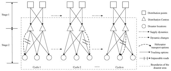
Figure 1.
Dynamic distribution system of multi-cycle emergency supplies under the three-tier distribution model.
3.1.2. Fundamental Assumptions
Considering the actual scenarios in disaster relief systems, the following fundamental assumptions are made to clarify the research questions.
Assumption 1.
It is assumed that there are sufficient emergency distribution tools available from the local government and community, that we can use vehicles and helicopters to transport supplies, and that road information or weather conditions are known, and that each type of transport equipment has the same specification and model.
Assumption 2.
The supplies depart at the same time as the start of each cycle, and supplies can be mixed for loading and transport, but there is no substitution between different kinds of supplies; there are waiting time indicators for the affected locations, and the psychological perception of the victims is based on the measurement of economic indicators, such as the loss of available supplies.
Assumption 3.
The demand for various materials is known for each affected location and the supply of materials at the distribution points is known, but the number of materials to be distributed to the multi-cycle disaster sites needs to be determined and we use 24 h as a relief cycle.
Assumption 4.
We allow a single distribution centre to supply multiple sites and each site can also receive supplies from multiple centres, but we are not considering inter-distribution of relief supplies between sites or between distribution centres at this time.
Assumption 5.
There is only one road from a distribution centre to a disaster site before the disaster, and we do not consider the cost of dispatching construction teams.
3.2. Time Constraints for Road Transport
After a large-scale earthquake, road damage and disruptions occur in the epicentre area, and the overall reliability of road access is generally impaired. Road travel times can be affected by factors such as road connectivity and damage conditions, while longer transport times can cause a reduction in satisfaction with relief efforts in the disaster area, as well as having a negative effect on the overall relief process. Therefore, it is vital to study road travel times after a disaster.
Considering the poor access to the road network in the disaster area and the occurrence of secondary disasters, the post-disaster roads will present three road conditions: passable, repairable and impassable. The road from distribution centre I to disaster site J in each relief cycle may be damaged, and some roads need to be repaired to meet the conditions of material transportation. The road travel time follows the formula below.
The length of road damage is ; the repair time per unit length of road is , r indicates the level of impact of different types of damage on the repair of each class of road and is taken as 1 here. is the coefficient of road damage and obstruction due to various disasters per cycle, called the road condition factor. It is generally used to measure the extent of road cracking and disruption caused by various primary and secondary disasters (aftershocks, rock falls, landslides, etc.).
, the value of closer to 1 represents the worse road condition, and its relationship with road rehabilitation and access speed is as follows. While , it means that the road is passable and does not need to be repaired, but the post-disaster vehicle speed is = , this equation represents the post-disaster vehicle speed limit. where represents the speed of transport vehicle from distribution centre to disaster point , and is the average speed from distribution centre to disaster point before the disaster. is a speed influence factor, , which increases as road rehabilitation conditions or navigation conditions turn better; While , it means that the road needs to be repaired, the speed limit is still satisfied after the repair is completed and we default that the road can be repaired within this cycle; While , it means the distribution centre to the affected point is severely damaged, the road is impassable, and the helicopter needs to be used to airlift the materials to the affected point. is the correction factor of helicopter travel distance to vehicle road travel distance, is the correction factor of helicopter speed to vehicle speed, and generally, . The above parameters are taken as and . To ensure safe post-disaster transport, the value of for post-disaster helicopter transport is 0.9, the value of is 0.8 when the road is in a passable and rehabilitated state, is taken as 1.5 and is taken as 2.
3.3. Integrated Perceptual Function Construction
After an earthquake, supplies are transported to each disaster site through the emergency logistics system. For the disaster sites, the quantity and timeliness of the arrival of supplies is the primary factor for the expected satisfaction of the disaster sites, while the difference in the arrival time and the quantity of supplies distributed among the sites is a triggering condition for the climbing effect and psychological imbalance caused by the limited rationality of the victims. In addition, if the supplies are damaged or fail during transportation due to poor transportation conditions or secondary disasters, as a result, the disaster areas receive damaged supplies, which will undoubtedly aggravate the suffering and despair in disaster areas and reduce satisfaction with relief [24]. Based on the above analysis, this study considers the cyclical psychological changes of disaster victims and constructs a comprehensive time perception satisfaction function and a comprehensive material loss distress effect to measure the psychological perception of people in disaster areas.
3.3.1. Comprehensive Time Perception Satisfaction
Time expectancy satisfaction and climbing effects are relatively abstract concepts, and we quantify the psychological state of disaster victims by introducing an exponential function.
When a disaster strikes, the distribution centres start rescuing the affected sites immediately. In view of the uncertainty of the transport conditions between the distribution centre and the disaster site after the disaster, and the variability in the perceived satisfaction with the relief time at the disaster site. For the disaster site, the victims hope that the supplies will reach the disaster area as soon as possible, and the victims have a psychological reference point for the expected time of arrival of supplies, but the arrival time has no realistic earliest delivery time limit. Therefore, research on time satisfaction in post-disaster emergency response is actually a one-sided soft time window scheduling problem. The satisfaction of the disaster site with the waiting time for supplies from each distribution centre is calculated by the following formula.
In the above equation, is the psychological expectation time of the victims of disaster point for each cycle of material transport, which is usually the time of arrival of the nearest distribution centre at that disaster point before the disaster; is the time taken for the material to arrive at the affected point and also the time taken to transport the material from distribution centre to the affected point by means of transport ; is the expected latest time per cycle for distribution centre to transport supplies to reach disaster point , generally the travel time from the furthest distribution centre to the disaster point before the disaster; is the quantity of material transported from distribution centre to affected point in cycle .
In Equation (3), when the material transportation time is before the psychological expectation time, the time satisfaction of the victims for this material transportation is 1; when the arrival time exceeds the latest time allowed to arrive in the disaster area, the expected time satisfaction of the victims drops to 0; when the arrival time is between the expected time and the latest time at the disaster site, the satisfaction of the waiting time in the disaster area decreases as the time increases, and the larger the time beyond the expectation, the faster the satisfaction decreases. is the disaster factor, which is used to measure the severity of the disaster in the affected area and can be expressed by indicators such as disaster intensity and disaster level. The greater the disaster factor, the more severely the area is affected, the more sensitive the victims are to the arrival time of supplies, and the faster the expected time satisfaction decreases. The value of is 1 in this paper.
In Equation (4), is the average value of time satisfaction for each arrival of supplies at disaster point , which represents the satisfaction of waiting time at disaster point in cycle .
Disaster sites are very sensitive to relief information, so the comprehensive post-disaster time satisfaction must include time climbing effects between sites. We then use the waiting time satisfaction and the climbing effect between disaster sites to construct a comprehensive time perception satisfaction at the disaster site. The specific construction process is as follows.
Equation (5) represents the time deviation rate of material arrival at disaster point in cycle . Equation (6) represents the level of time climbing effect at disaster point .
In Equation (6), , the smaller the value of , the smaller the time climbing effect between disaster points in cycle t and the greater the fairness of rescue arrival times, then the lower the probability of causing irrational behaviour after a disaster.
Combine all of the analysis in Section 3.3.1 above. we construct the comprehensive time-perceived satisfaction of disaster point as in Equation (7).
Then the multi-period and multi-hazard comprehensive time perceived satisfaction is as in Equation (8). is the first objective function in this paper.
3.3.2. Comprehensive Material Loss Perceived Pain Effect
Potential static demand for emergency supplies existed at each disaster site before the disaster, which did not actually exist. When a disaster occurs, the potential demand for emergency supplies is immediately transformed into a realistic demand for supplies, and the demand for emergency supplies surges within a short period of time after the disaster, which in turn leads to the total supply of supplies from the distribution centre not being able to meet the total demand for supplies at each affected site. Due to the limited rationality of the affected population, there will also be a material comparison effect between the disaster sites. If materials are damaged in transport, receiving the damaged materials will reduce the satisfaction of the affected population with the materials and even trigger a huge public reaction. This can be seen in the negative feedback that some communities received when they received spoiled supplies in the early days of the COVID-19 epidemic in Shanghai. Therefore, this paper constructs a comprehensive material loss function for the disaster site based on the unmet amount of material at the disaster site, the comparison effect and the material damage pain effect. The function construction process is as follows.
Equation (9) represents the amount of material unsatisfied at affected point ; Equation (10) represents the material unmet loss at affected point , where the marginal perceived loss in material unmet increases as the amount of material unmet increases. In Equation (10), indicates the vulnerability of the affected point , which mainly depends on the location, personnel composition, building structure and mitigation capacity of the affected point, etc. In this paper, the value of is taken as all 1; is the utility of emergency material to affected point in cycle . The utility of different materials varies according to objective post-disaster realities. Equation (11) represents the comparison loss of affected point , which measures the level of fairness in material distribution among affected points, , and the larger is, the stronger the comparison effect of affected point , resulting in a stronger psychological relative exploitation loss among disaster points. When material damage is not considered, we define the combined material loss effect at the affected point as in Equation (12).
Equation (12) represents the combined material unsatisfied loss at affected point , which is more representative of the relationship between material unsatisfied loss and comparison loss.
However, the post-disaster transport environment is complex, and materials are highly susceptible to damage through the processes of loading, unloading, handling and distribution, so the damage to materials should be taken into account in studies of the psychological pain of material loss in disaster areas. We use the prospect theory to describe the psychological distress effect of damage to emergency supplies at the affected point . The construction process is as follows.
Equation (13) is the damage rate of material e at affected point . Each affected point wants to receive undamaged material, therefore, the reference point of material destruction at each affected point is 0. Then the psychological distress effect of material damage at affected point is as in Equation (14).
In Equation (14), is the deviation of the true value of the target that the disaster victims are concerned about from the psychological reference point, where is the risk parameter, and ; , which means that the affected point is averse to material damage, and the larger is, the more averse the disaster victims are to loss.
Thus, the combined material loss effect for a multi-cycle multi-hazard site is shown in Equation (15). is the second objective function in this paper.
3.4. Total Cost of Post-Earthquake Relief
The total cost of post-earthquake relief includes three components: the cost of raising supplies, the cost of transportation and the cost of repairing roads in the earthquake area.
- (1)
- Material raising and transportation cost.
- (2)
- Road rehabilitation costs.
The total rescue cost is shown in Equation (18).
represents both the total multi-cycle cost and the third objective function of this paper.
4. Emergency Material Distribution Transport Model
4.1. Notations
Sets, parameters, and decision variables of the model are described as follows:
- (1)
- Mathematical sets
is the set of emergency material collection and distribution points, ;
is the set of emergency material distribution centres, ;
is the set of affected points, ;
is the set of periods, ;
is the set of transport vehicles: is the set of transport vehicles: , which represents the set of all transport vehicles, where = represents the set of vehicle transport and represents the set of helicopter transport.
is the set of material types, ;
- (2)
- Parameters
Some of these parameters have already been defined in the previous section on function construction and will not be repeated here.
Time parameters.
: the earliest moment in cycle when transport vehicle is used to start transporting materials from material distribution centre to disaster site .
: the time it takes for the supplies to reach the disaster site and the time taken in cycle to transport emergency supplies from distribution centre to disaster site by transport mode . In this paper, we assume that the earliest moment of rescue starts as moment 0, so that is the moment of arrival at disaster point .
: the moment in cycle when disaster point has fully received relief supplies from distribution centre .
: the psychological expected transit time at affected point for the arrival of supplies per cycle, generally from the nearest pre-disaster distribution centre to the disaster site.
: the latest time that transported material reaches disaster point per cycle, generally the time that the furthest distribution centre reaches the disaster point before the disaster.
: the latest expected arrival time of supplies at disaster point per cycle. Considering the realistic transportation conditions after a disaster, this paper takes = 1.5 as the longest time tolerated by the disaster area. if the time of a particular transport exceeds that time, then the perceived satisfaction of time to reach disaster point is zero.
Cost parameters.
: the cost per unit of material raised for emergency material in cycle .
: the fixed transportation cost from distribution point to distribution centre in cycle .
: the fixed transportation cost from distribution centre to disaster point in cycle .
: the cost of rehabilitation per unit length of road.
: the unit cost of transporting emergency material from emergency material distribution point to distribution centre in cycle .
Material parameters.
: the latest supply of material at distribution point in cycle .
: the quantity of material left in stock at the end of cycle at the distribution point .
: the number of deliveries of material from distribution point to distribution centre in cycle .
: the maximum volume of transport of material from distribution point to distribution centre in cycle , generally the total stock of material at the distribution point.
: the stock of material remaining in distribution centre at the end of cycle .
: the quantity of material transported from distribution centre to disaster point in cycle .
: the maximum volume of material to be delivered from distribution centre to disaster point in cycle ; when material is in short supply, it is generally the total reserve of material in distribution centre .
: the initial predicted demand for emergency supplies at the disaster point in cycle .
: the shortage of emergency supplies at disaster point in cycle ; and the number of unmet supplies in the current cycle is converted into the next cycle’s supply requirements.
: the quantity of damaged material generated in cycle when material is transported from distribution centre to affected point . If , then ; if , then ; if , then . Damaged material from transport in the current cycle is converted to material requirements for the next cycle. τ is the material damage adjustment factor and takes the value of 0.1 and assumes that there is no material damage in the last cycle.
: the actual demand for emergency supplies at the disaster point in cycle . if , ; when , .
Other parameters.
: the shortest distance between the distribution point and the distribution centre . This section of road is on the outside of the affected area, so there is no road damage on this road, and the transport vehicles deliver the supplies to the distribution centre in the shortest possible distance.
: the distance between distribution centre and disaster point . This section of road is in the affected area and exists with road damage and repairs.
: the minimum emergency material security rate at the disaster point, and if the material security rate falls below this value, it may induce irrational behaviour among the affected population.
- (3)
- Decision variables
: If supplies are delivered from distribution point to distribution centre in cycle , the value of is 1. otherwise, the value of is 0.
: If supplies are delivered from distribution centre to distribution point in cycle , the value of is 1. otherwise, the value of is 0.
4.2. The Proposed Model
Based on the above analysis and model constraints, the multi-cycle emergency material dispatch model constructed in this paper is as follows.
- (1)
- Objective functions
The objective function (19) represents maximising the comprehensive perceived time satisfaction for all disaster points in all cycles; Equation (20) represents minimising the comprehensive material loss pain effect for all disaster points in all cycles; Equation (21) represents minimising the total post-disaster relief costs for all cycles, including transport costs and road repair costs etc.
- (2)
- The constraints
Equation (22) balances the amount of material shortage and depletion at each disaster point. Equation (23) ensures that the flow of materials from the distribution centre is conserved and also ensures that if materials are distributed in excess of demand in one cycle are carried over to the next cycle for distribution. Equation (24) ensures that the flow of material from the distribution point is conserved and that the amount of material transported from the distribution point to the distribution centre does not exceed the amount of material available at the distribution point during the cycle. Equations (25) and (26) represent the maximum capacity constraints for distribution points and distribution centres respectively. Equation (27) represents the amount of material delivered by each distribution centre to the disaster point that does not exceed the demand at the disaster point, and also constrains the amount of material delivered to the disaster point to not fall below the minimum material limit. Equation (28) is the moment in cycle when disaster point has fully received relief supplies e from distribution centre . Equation (29) is a 0–1 constraint on the material delivery decision variable; Equation (30) is a non-negative constraint on the material variable.
5. Improved NSGA-II Algorithm
The multi-objective emergency resource allocation model constructed by Equations (19)–(30) is a non-linear mixed integer programming model, which covers multiple cycles, multiple disaster areas, multiple supplies and transportation modes. For multi-objective optimisation problems, if the multi-objective problem needs to be transformed into a single-objective problem, scholars often use methods such as the linear weighting method, the minimal-extreme method and the -constraint method [25]. However, the value of the multi-objective function weights is influenced by the subjective will of the decision maker, the model in this paper has more relevant parameters and constraints, the solution complexity is larger, and there may be negative correlation between each objective function in the multi-objective optimisation process, and the solution is often a set of non-inferior solutions, so there is no optimal solution that satisfies all objectives at the same time. Therefore, considering the complexity of the model and the realistic post-disaster scenario, we designed an improved non-dominated ranking multi-objective genetic algorithm to solve the model.
5.1. Improved NSGA-II Algorithm Steps and Strategies
In this paper, the steps for designing a genetic algorithm with an elite retention strategy for non-dominated sorting are as follows.
- 1.
- Chromosomal coding. This paper uses real number coding to describe the amount of material distributed from the distribution centre to the disaster site each cycle. Let the matrix be a solution in the target solution space and the matrix column vector , the number of matrix rows represents the distribution centre , the number of matrix columns represents the disaster point , and the chromosome-encoded genes are represented by the vector = , , , ]. , for , there is a supply of emergency supplies in cycle . If , it represents the supply of relief supplies from distribution centre to disaster point in cycle . If , it represents its non-participation in the relief of disaster point ; the coding gene within the vector represents the quantity of the corresponding kind of material transported by distribution centre disaster point , , where , .
- 2.
- Generating the initial population . Initial population parameters such as , , and have an impact on the algorithm’s ability to find the best and the iteration efficiency. In order to ensure the goodness of the initial population, the initial population is first generated randomly and uniformly according to certain constraints for each gene value, and then the initial population is formed after gradually implementing the coding correction strategy, and then the generalized reverse learning strategy is used to form the generalized population . After the coding correction, the initial population is combined with the generalized population , and the top individuals with better adaptability are selected to form the initial population through non-dominated sorting and crowdedness comparison.
5.1.1. Infeasible Coding Scheme
The chromosome coding matrix corresponds to each material distribution scheme, and for , material is issued in a parallel distribution relationship, with each chromosome changing and generating a new scheme after initialisation, crossover and mutation of the coding genes. The infeasible solutions in this paper mainly violate the constraints of Equations (26) and (27), and the following scenarios can result in unequal distribution of resources, weaken the fairness of material distribution or produce infeasible solutions.
- 1.
- For each column of the coding matrix, if and , and , which means that the amount of material allocated to the disaster point by all distribution centres is greater than the actual demand, which will both violate the constraint and cause uneven distribution of material when material is in short supply, and weaken the fairness among disaster points, resulting in an infeasible distribution scheme.
- 2.
- For each column of the coding matrix, if and , and , which means that the total amount of relief supplies from all distribution centres cannot meet the minimum emergency supply demands at the disaster point, which violates the minimum supply satisfaction constraint and makes this distribution scheme infeasible.
- 3.
- For each row of the coding matrix, if and , and , then the amount of material distributed by distribution centre to disaster point in cycle t is greater than its maximum allocable amount, resulting in an emergency material conflict and thus an infeasible solution.
5.1.2. Coding Correction Strategy
The code correction strategy is to eliminate conflicts between supply and demand in the distribution of materials, make the code legal and achieve effective response of the distribution centre to the demand for materials at the disaster point, so as to meet the minimum demand as well as not to exceed the actual demand, and at the same time, if the supply of materials owned by the distribution centre is finished, it will no longer respond to the demand for materials at the disaster point. means the remaining stock of material in distribution centre in cycle . For , , when there is no material distribution, .
The coding correction strategy is as follows.
Step 1: For the matrix A to be corrected, choose an unchecked column (i.e., the affected point ) at random, where .
Step 1.1: For distribution centre that satisfies , , , execute .
Step 1.2: If and , for the materiel in dimension e, sort the materiel in ascending order by the ratio, and for the minimum distribution point , execute , while the corresponding distribution centre * material remaining in stock .
Repeat the above steps until for that holds.
Step 1.3: If and , then choose and do not participate in transport point to start material distribution. Execute and the material surplus at that point is .
Repeat the above steps until for that holds.
Step 2: If all columns are corrected (i.e., all disaster points have been distributed with supplies), then the coding correction is complete; otherwise, go to step 1 to continue with the coding correction.
5.1.3. Generalized Reverse Learning Strategy
In this paper, a generalized reverse learning strategy is used to initialize the population, with the following definitions. Assuming that and that is in space , transform into in -space by Equation (31).
where and , but may go beyond the space and become an invalid solution, at which point is corrected according to Equation (32).
Following the above steps, when the strategy is executed for the encoding matrix, we have in an n-dimensional space, where is a real number between the intervals , and for , o , , where , and again correcting for out of range . The corresponding generalized populations can be generated by executing the above strategy on the chromosome matrix.
5.1.4. Constructing the Fitness Function
In this paper, in order to facilitate the non-dominated sorting process, the target function is taken as the inverse transformed fitness function, , and the target functions and are directly adopted as the fitness functions, , .
5.1.5. Construction of Non-Dominated Sorted Solution Sets
We use the fitness functions , , to perform a non-dominated sorting operation, where each individual in the population has attributes , , is the number of individuals dominating in the population, and is the set of individuals dominated by . The following steps are performed.
- 1.
- First, we identify the individuals in the population whose is 0 and place them in the non-dominated set .
- 2.
- Second, we traverse the set dominated by individual in set and perform for individual in and if , deposit the individual in another set .
- 3.
- Third, take as the first level of the set of non-dominated individuals, make the = 1 of the non-dominated order of individuals in rank, and continue to perform the corresponding hierarchical operation on the set and assign the corresponding non-dominated order, when all individuals are hierarchically ranked, stop the hierarchical sorting operation.
5.1.6. Crowding Distance and Crowding Comparison Operator
The crowding distance, which is important for maintaining population diversity, is calculated as follows.
- 1.
- For each individual currently, let the crowding distance , .
- 2.
- We sort the populations in ascending order for individuals in the same rank, based on the objective function value .
- 3.
- For individuals at the edge of each class, let the crowding distance be infinity and .
- 4.
- For individual in the middle of each rank, the crowding distance is calculated by Equation (33).
In Equation (33), denotes the crowding degree of individual , and are the jth objective function values of individual and , and and are the maximum and minimum values of the corresponding objective functions.
Crowding comparison: Individuals are given the non-dominated order and the crowding distance after the non-dominated ranking and crowding calculation. For any two individuals and , when the following conditions are satisfied, individual is judged to be in the dominant position.
- 1.
- If , then individual is in a dominant position.
- 2.
- If and , then individual is dominant.
5.1.7. Improved Elite Retention Strategy
If all individuals of rank are retained in the new parent set, the number of individuals in the set is less than , and after all individuals of rank are retained, the number of individuals in the new parent set is greater than . At this time, the crowding degree is calculated for the individuals of rank and descending order is executed to delete the individuals with the worst crowding degree of that rank. Then the crowding level is recalculated, and the above operation is repeated to remove the worst crowded individuals until the sum of the retained individuals at that level and the number of individuals in the previous levels is .
5.1.8. Improved Genetic Manipulation
- 1.
- Selection. In this paper, we use a binary tournament selection strategy, where the individual with the smaller non-dominance rank is preferred when two individuals are compared; if both individuals have the same non-dominance rank, the individual with the greater crowding is preferred.
- 2.
- Crossover. The chromosome adaptive crossover probability is calculated based on the equation , where and are the maximum and minimum crossover probabilities, is the number of iterations and is the maximum number of iterations. if , perform a simulated binary crossover, while the adaptive crossover probability becomes progressively smaller with each iteration, allowing the algorithm to focus on the global search in the early stages and gradually on the local search in the later stages.
- 3.
- Mutation. We use operations such as adaptive mutation probability, polynomial variation, and generalized reverse learning to improve the local search capability of the algorithm, and to maintain population diversity.
- (1)
- Adaptive mutation probability. we calculate the probability of chromosomal variation based on the equation , where and are the maximum and minimum mutation probabilities, and this equation gradually increases the probability of chromosomal mutation in the late iterations to increase population diversity.
- (2)
- Mutation operation. if , perform the generalized polynomial mutation operation, and perform the generalized reverse learning operation on the polynomially mutated individual. after executing the reverse learning operation for . times, combine the generalized mutation solution with the original mutation solution; then, after non-dominated sorting, select the best solution to replace the original mutation solution. Thus, we can obtain the better individual after the mutation.
5.1.9. Iteration and Termination
If , continue the iteration operation; otherwise, end all loop iterations and output all feasible solutions including the Pareto optimal solution.
5.2. INSGA-II Algorithm Flow Chart
The flowchart of the Improved Non-Dominated Sorting Genetic Algorithm (INSGA-II) is shown in Figure 2.
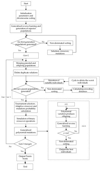
Figure 2.
The flowchart of improved non-dominated sorting genetic algorithm (INSGA-II).
6. Case Experiments and Analysis
6.1. Experimental Examples
Our numerical data is based on the literature study by Wang Yanyan et al. [26]. The overall context is the 2008 Wenchuan earthquake, using a combination of actual and simulated data. We selected three areas severely affected by the earthquake, Wenchuan County (), Beichuan County () and Shifang City (), as the disaster locations, Deyang city (), Chengdu city () and Mianyang city (), which have a good economic base, were selected as the three distribution centres for emergency supplies; Xi’an City () and Wuhan City (), which are relatively close to the national emergency supplies reserve, were selected as the distribution points for supplies, in order to study the distribution of tents (), blankets () and drinking water (), which are in short supply in post-disaster disaster areas. This creates three disaster locations, and that three emergency distribution centres support the disaster locations with supplies after the disaster, while three emergency supplies of tents, blankets and drinking water are delivered from two distribution points to each distribution centre. The cost of raising the three types of supplies at the distribution point is RMB 500, RMB 50 and RMB 20 respectively. Taking one day (24 h) as a cycle, we study the distribution of emergency supplies for the first four cycles of disaster emergency relief, and the amount of emergency supplies supplied at the distribution point for each cycle is shown in Table 1. The shortest distance, fixed cost and unit cost from distribution point H to distribution centre i are shown in Table 2. The initial material availability (, , ) at the distribution centre is (1000, 1200, 1500), (1000, 1500, 1200) and (1200, 2000, 2500). Information on the disaster situation is reported for each cycle, and the distance and cost information from the distribution centre to the disaster point and the demand for supplies at the disaster point are shown in Table 3 and Table 4 respectively. The average speed of a rescue vehicle when travelling normally is 80 km/h, the average speed of a relief helicopter is 150 km/h and the unit transport cost of a helicopter is 5 RMB/km. Roads in the disaster area are damaged by primary and secondary hazards, and the road transport conditions in the disaster area are given by the relevant experts after each cycle of assessment, and the road condition coefficients and damage distances between the distribution centre to and the disaster point are shown in Table 5. The utility values of the different types of emergency supplies to the disaster points for each cycle are shown in Table 6. In this paper we set a unit road repair time of 0.1 h/km, a minimum material requirement guarantee rate of 0.55, the value of was taken as 0.88 and the value of as 2.25.

Table 1.
Supply of emergency supplies per cycle of distribution points *.
Table 2.
Information on the shortest distance from distribution point H to distribution centre I and the associated costs *.
Table 3.
Distance and cost information from distribution centre I to disaster point J *.
Table 4.
Initial estimated material demands for each cycle of the disaster point.
Table 5.
Road condition coefficient and damage length information *.
Table 6.
Utility values for different emergency supplies at each cycle of the disaster.
6.2. Experimental Setting and Analysis of Results
Based on the proposed model and the designed algorithm, the case was calculated using Matlab R2019b software programming on a hardware running environment of Intel(R) Core(TM) i5-6300HQ@2.30GHz with 16 GB RAM and software running environment of Window10 64-bit operating system computer. The algorithm parameters were set to a population size () as 100, a maximum number of iterations () as 1000, a crossover probability () as 0.7, a crossover probability () as 0.2, a mutation probability () as 0.1, a mutation probability () as 0.01, and as 10. In order to compare the computational results of several algorithms objectively, we compare the results of INSGA-II, NSGA-II, SPEA-II and MOPSO algorithm runs under the condition that the algorithm parameters are consistent as far as possible. The values of several algorithm parameters are basically the same, and the number of populations of each algorithm is set to 100 and the iterations are set to 1000. To verify the accuracy of the algorithm search results, we performed 20 sets of replicate tests and recorded the optimal values of each target (, ) in the iterations, and the calculated results are shown in Table 7.
Table 7.
Comparison of calculation results of improved NSGA-II with other algorithms *.
We can calculate the mean value of the optimal value of each indicator for several times to compare the algorithms in terms of solution accuracy, and we can also judge the difference in convergence stability of different algorithms by calculating the variance of the optimal value of each indicator for several times, and the specific results of the mean value and variance of the optimal value obtained from 20 runs of different algorithms are shown in Table 7. We can learn the following information from the mean values calculated from the above 20 comparative tests of the optimal values of each target., the improved algorithm in this paper reduces the satisfaction transformation index by 8.21%, 1.05% and 6.26% respectively, that is, it increases the satisfaction index by 8.21%, 1.05% and 6.26% respectively; it reduces the perceived loss index by 14.83%, 1.74% and 20.25%; it reduces the total scheduling cost by 1.77%, 0.53% and 3.31%, From the above three optimisation metrics, we can judge that the improved algorithm outperforms the other three algorithms in terms of solution accuracy. We know from the variance obtained from multiple calculations that the variance of the improved algorithm is smaller than the other three algorithms for the optimal values of the three indicators, so we can judge that the stability of the improved NSGA-II algorithm in this paper is better than the other three algorithms in every metric. In summary, the improved NSGA-II algorithm in this paper outperforms the other three comparative algorithms in terms of solution accuracy and algorithm stability.
6.3. Performance Comparison of Four Optimisation Algorithms
We compare the calculation results of INSGA-II algorithm, NSGA-II algorithm, SPEA-II algorithm and MOPSO algorithm, and the distribution of the iterative Pareto front target space of several algorithms is shown in Figure 3.
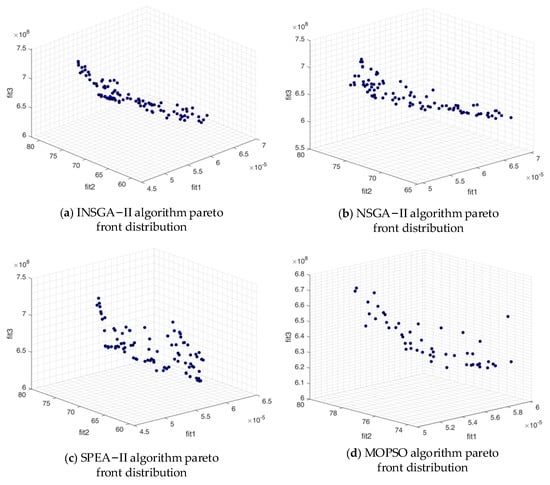
Figure 3.
Distribution of Pareto front for four intelligent optimisation algorithms.
We can see from the iterative images of the four algorithms that all four algorithms can find feasible solutions and converge to the Pareto front, and the solutions of the INSGA-II and NSGA-II algorithms for the front are significantly more uniform than those of the SPEA-II and MOPSO algorithms. However, the specific performance of each algorithm cannot be intuitively seen from the above Pareto images. In order to measure the performance of the INSGA-II algorithm exactly, this paper uses the Convergence Performance (), the Spacing Performance (), and the Hypervolume () to compare and analyse the algorithms.
The Convergence Performance (): This indicator measures the degree of fit between the set of fronts of solutions obtained by the algorithm and the set of true optimal pareto fronts, as shown in the following equation. In Equation (31), is the minimum Euclidean distance between solution and the optimal solution set, is the number of solution sets in the resulting Pareto set, and the smaller the value of the , the closer the resulting solution set is to the true Pareto optimal solution set.
The Spacing Performance (): This indicator measures the degree of uniformity in the distribution of individual solution sets and is calculated by Equation (32). In the following equation, means the minimum distance from the ith solution to the other solutions in the resulting solution set, and means the average of the minimum distances. the smaller the value of the , the more evenly distributed the resulting solution set is.
The Hypervolume (): This metric measures the comprehensive performance of the solution set. The more solutions and dispersion in the solution set obtained by the algorithm, the greater the value of the , which is calculated as shown in the following equation. Equation (33) means the hypervolume space formed between the solution and the reference point in the solution set .
When calculating each of the above indicators it is necessary to calculate the Euclidean distance di between different solution sets in the -dimensional space, which is calculated according to the following equation.
In order to eliminate the influence of chance factors in the calculation of the algorithms, we ran both INSGA-II and the comparison algorithms 10 times and took the average of each metric to measure the specific performance of each algorithm, and the calculation results are shown in Table 8.
Table 8.
Different performance indicator values for four algorithms.
We can obtain the data values calculated from the various algorithm performance indicators in Table 8, whether in terms of the convergence performance , the spacing performance , or the comprehensive index of the algorithm, the INSGA-II algorithm in this paper shows better performance than other algorithms, and also shows that the improvement strategy is effective for the NSGA-II algorithm in this paper.
6.4. Choice of Material Distribution Options
The post-disaster emergency relief decisions should be based on consideration of the comprehensive psychological perceptions of the victims, as well as improving their psychological satisfaction, reducing perceived losses and avoiding triggering irrational behaviour, thereby improving the overall effectiveness of multi-cycle emergency relief. As this paper is a multi-objective scheduling model, there is a large difference in the overall satisfaction, overall material loss and cost levels obtained from different scheduling options, so we propose an option selection method. In one iteration, the INSGA-II algorithm obtained a total of 100 feasible solutions, all of which converged to the Pareto front surface, from which three typical optimal solutions were selected: the time-aware optimal solution, the material loss-aware optimal solution, and the cost-optimal solution as shown in the Table 9.
Table 9.
Typical Pareto optimal solution.
In the distribution scheme selection, fit1 measures the satisfaction of the disaster area, and the smaller the , the greater the satisfaction; is the perceived loss of the disaster victims, and the smaller its value, the better;
is the cost of relief, and its value is also the smaller, the better. The specific scheme selection indicators are as follows.
Time satisfaction indicator:
Perceived loss indicator:
Cost Indicator:
In the above equation, and are the maximum and minimum values of for all solutions, and . is the value for solution (). From this, the values of the corresponding selection indicators can be calculated for each option. As the effectiveness of disaster relief is based on the “people-centred” principle, it is necessary to consider the psychological behaviour of the victims at the early stage of the disaster and weaken the economic indicators to avoid the irrational behaviour of the victims due to psychological breakdown, therefore, it is considered to set the time perceived satisfaction and loss perception as the evaluation criteria and combine the satisfaction and loss indicators to assist the decision-making; as the transportation of supplies to the disaster area gradually increases in the later stage of rescue, we need to consider time and cost indicators, combine time satisfaction indicators and cost indicators, weaken the perceived loss indicators, and select the corresponding distribution scheme based on the comprehensive assessment of decision makers and the acceptance of each indicator in the specific scheme selection.
In the following, we give specific allocation options under the decision maker’s preferences based on the above selection method.
If the decision maker delivers emergency supplies at all costs, based on the perspective of time urgency and the psychological perceived loss of the victims, the decision maker expects that the victims’ perceived satisfaction with time will reach 80% and the perceived loss of supplies will not exceed 40%, in this case, we use Equations (38) and (39), and combine them with the resulting pareto frontier to select an allocation scheme that satisfies the requirements, as shown in Table 10 for allocation scheme 1; If the decision maker takes a cost perspective, such as the decision maker expects that the victims’ perceived satisfaction with time will reach 60% and the comprehensive cost does not exceed 70%, in this case, we can use Equations (39) and (40) and combine them with the resulting pareto frontier to arrive at a feasible solution that satisfies the requirements, as shown in Table 10 for allocation scheme 2. As a result, the decision maker can select the appropriate material dispatch plan based on their own preferences and the perception of the disaster victims, while the rational dispatch of multi-cycle materials increases the continuity and sustainability of post-disaster emergency relief.
Table 10.
Distribution schemes preferred by decision makers.
7. Conclusions and Discussion
This paper is based on the realistic background of large-scale emergency emergencies. On the basis of objective factors such as poor road transport, material shortage and multimodal transport, it combines the subjective psychological behavioural factors of the victims to optimise the multi-cycle emergency material distribution problem after the disaster. By considering a variety of limited rational psychological factors, we construct multiple psychological perception functions to avoid the deviation of emergency relief from the most intuitive feelings of the victims. For example, we consider the impact of the waiting effect and the comparison effect on the psychological perception of the victims and construct a comprehensive time satisfaction function; we consider the amount of unsatisfied supplies, the comparison effect of supplies at the disaster site and the painful effect of damage to supplies to construct a comprehensive perception of supplies in the disaster area satisfaction. We designed and improved the NSGA-II algorithm to solve the constructed model and proposed a material allocation scheme selection strategy with decision maker preferences, which provides a solution for the sustainable supply and deployment of materials for multi-cycle relief after a disaster. The results show that the multi-objective model developed in this paper is suitable for solving the post-disaster multi-cycle emergency material distribution problem, and the improved NSGA-II algorithm has superior solution performance than other algorithms.
However, This paper only considers the impact of road conditions on transportation time from a temporal perspective, and constructs a comprehensive perceptual function for a specific scenario to solve the problem of distribution of emergency supplies, but lacks time-varying considerations of the scope of the disaster area based on a spatial perspective, such as the scenario where the scope of the disaster area is expanded and secondary disasters lead to the intensification of the disaster situation at the affected sites. Moreover, this paper only studies the multi-cycle distribution of emergency supplies under a deterministic supply-demand relationship, without considering the ambiguous and dynamically changing situation of post-disaster demand. In view of the objective reality of fuzzy demand information in disaster areas, theories such as fuzzy theory and interval number can be introduced to portray demand information, and then combined with objective reality constraints and subjective psychological behavioural factors of disaster victims, the combination of subjective and objective factors can jointly study the multi-cycle emergency material dispatching problem under the condition of fuzzy demand after disaster, and this research perspective may be the next research direction of emergency material distribution after disaster.
Author Contributions
Conceptualization, F.W.; Funding acquisition, F.W. and Y.L.; Investigation, F.W., X.G., Y.L. and W.Z.; Methodology, F.W., X.G., Y.L. and W.Z.; Project administration, X.G. and W.Z.; Writing—original draft, X.G.; Writing—review & editing, X.G. and J.Z. All authors have read and agreed to the published version of the manuscript.
Funding
This research was funded by National Natural Science Foundation of China (Grant No. 71872002; Grant No. 72274001), Major Project on Humanities and Social Sciences Research in Anhui Universities (Grant No. SK2020ZD16).
Institutional Review Board Statement
Not applicable.
Informed Consent Statement
Not applicable.
Data Availability Statement
Not applicable.
Conflicts of Interest
The authors declare no conflict of interest.
References
- Knott, R.J.D. The logistics of bulk relief supplies. Disasters 1987, 11, 113–115. [Google Scholar] [CrossRef]
- Ray, J. A multi-period linear programming model for optimally scheduling the distribution of food-aid in West Africa. Ph.D. Thesis, University of Tennessee, Knoxville, TN, USA, 1987. [Google Scholar]
- Haghani, A.; Oh, S.-C. Formulation and solution of a multi-commodity, multi-modal network flow model for disaster relief operations. Transp. Res. Part A Policy Pract. 1996, 30, 231–250. [Google Scholar]
- Haghani, S.C.O.A. Testing and evaluation of a multi-commodity multi-modal network flow model for disaster relief management. J. Adv. Transp. 1997, 31, 249–282. [Google Scholar] [CrossRef]
- Barbarosoǧlu, G.; Arda, Y. A two-stage stochastic programming framework for transportation planning in disaster response. J. Oper. Res. Soc. 2004, 55, 43–53. [Google Scholar] [CrossRef]
- Ma, Z.; Wang, S. A Multi-Stage and Dynamic Multi-Modal Transportation Model for Relief Commodities in Natural Disasters. In Proceedings of the 11th Chinese Annual Conference on Management Science, Chengdu, China, 16–19 October 2009; pp. 59–64. [Google Scholar]
- Zhu, J.; Huang, J.; Liu, D.; Han, J. Randomized Algorithm for Vehicle Routing Model for Medical Supplies in Large-Scale Emergencies. Oper. Res. Manag. Sci. 2010, 19, 9–14. [Google Scholar]
- Liu, C.; He, J.; Shi, J. The Study on Optimal Model for a Kind of Emergency Material Dispatch Problem. Chin. J. Manag. Sci. 2001, 3, 30–37. [Google Scholar]
- Sheu, J.-B.; Pan, C. A method for designing centralized emergency supply network to respond to large-scale natural disasters. Transp. Res. Part B Methodol. 2014, 67, 284–305. [Google Scholar] [CrossRef]
- Du, L.; Li, X.; Gan, Y.; Leng, K. Optimal Model and Algorithm of Medical Materials Delivery Drone Routing Problem under Major Public Health Emergencies. Sustainability 2022, 14, 4651. [Google Scholar] [CrossRef]
- Bodaghi, B.; Palaneeswaran, E.; Abbasi, B. Bi-objective multi-resource scheduling problem for emergency relief operations. Prod. Plan. Control. 2018, 29, 1191–1206. [Google Scholar] [CrossRef]
- Kovács, G.; Spens, K.M. Humanitarian logistics in disaster relief operations. Int. J. Phys. Distrib. Logist. Manag. 2007, 37, 99–114. [Google Scholar] [CrossRef]
- Ge, H.; Liu, N.; Zhang, G.; Yu, H. A model for distribution of multiple emergency commodities to multiple affected areas based on loss of victims of calamity. J. Syst. Manag. 2010, 19, 541–545. [Google Scholar]
- Wang, X.; Zhang, N.; Zhan, H. Emergency material allocation model considering the non-rational psychological comparison of the victims. Chin. J. Manag. 2016, 13, 1075–1080. [Google Scholar]
- Chen, Y.-x.; Tadikamalla, P.R.; Shang, J.; Song, Y. Supply allocation: Bi-level programming and differential evolution algorithm for Natural Disaster Relief. Clust. Comput. 2020, 23, 203–217. [Google Scholar] [CrossRef]
- Wang, L.; Zhou, X.; Zhao, Z.; Liu, L.; Yu, L. Integrated decision making of emergency vehicle allocation and emergency material distribution. J. Cent. South Univ. Sci. Technol. 2018, 49, 2766–2775. [Google Scholar]
- Song, Y.; Huang, X.; Ma, Y.; Li, M. Emergency resource allocation considering psychological pain effect of disaster victims under multi-dimensional fairness measurement. J. Saf. Sci. Technol. 2021, 17, 47–53. [Google Scholar]
- Chen, Y.; Zhao, Q. The model and algorithm for emergency supplies distribution based on fairness. Syst. Eng. -Theory Pract. 2015, 35, 3065–3073. [Google Scholar]
- Chen, G.; Fu, J. Multi-Objective Emergency Resources Allocation with Fairness and Efficiency Considerations. Chin. J. Manag. 2018, 15, 459–466. [Google Scholar]
- Li, Y.; Ye, C.; Ren, J.; Tang, T.; Guo, J. Multi-cycle emergency medical material allocation considering patient panic in epidemic environment. J. Saf. Environ. 2021, 21, 1643–1651. [Google Scholar]
- Zheng, B.; Ma, Z.; Li, S. Integrated optimization of emergency logistics systems for post-earthquake initial stage based on bi-level programming. J. Syst. Eng. 2014, 29, 113–125. [Google Scholar]
- Wang, H.; Wang, J.; Ma, S. Decision-making for emergency materials dynamic dispatching based on fuzzy demand and supply. Chin. J. Manag. Sci. 2014, 22, 55–64. [Google Scholar]
- Sheu, J.-B. An emergency logistics distribution approach for quick response to urgent relief demand in disasters. Transp. Res. Part E Logist. Transp. Rev. 2007, 43, 687–709. [Google Scholar] [CrossRef]
- Wang, Y. An Optimization Method for Distributing Emergency Materials Which Balances Multiple Decision Criteria. Processes 2022, 10, 2317. [Google Scholar] [CrossRef]
- Abdolhamid, Z.; Mehrdad, K.; Husseinzadeh, K.A. Multi-objective decision-making model for distribution planning of goods and routing of vehicles in emergency multi-objective decision-making model for distribution planning of goods and routing of vehicles in emergency. Int. J. Disaster Risk Reduct. 2020, 48, 101587. [Google Scholar]
- Wang, Y.; Sun, B. Dynamic Multi-stage Allocation Model of Emergency Materials for Multiple Disaster Sites. Chin. J. Manag. Sci. 2019, 27, 138–147. [Google Scholar]
Disclaimer/Publisher’s Note: The statements, opinions and data contained in all publications are solely those of the individual author(s) and contributor(s) and not of MDPI and/or the editor(s). MDPI and/or the editor(s) disclaim responsibility for any injury to people or property resulting from any ideas, methods, instructions or products referred to in the content. |
© 2023 by the authors. Licensee MDPI, Basel, Switzerland. This article is an open access article distributed under the terms and conditions of the Creative Commons Attribution (CC BY) license (https://creativecommons.org/licenses/by/4.0/).